Chapter 7: Multiple Imputation Case Studies

Chapter 7 presents two case studies typical of “real world” data analysis projects. Data from the 2006 Health and Retirement Study (HRS; available at http://hrsonline.isr.umich.edu/) and a longitudinal seizure counts data set downloaded from Johns Hopkins University (available at http://www.biostat.jhsph.edu/~fdominic/teaching/LDA/lda.html; Thall and Vail [1990]) are used in the examples.

7.2 Comparative Analysis of HRS 2006 Data Using Complete Case Analysis and Multiple Imputation of Missing Data

This first case study is based on data from the 2006 HRS. The HRS is a longitudinal panel study that surveys a representative sample of Americans over the age of 50 every 2 years. Although by design HRS is a longitudinal survey, we use data from only the 2006 data collection wave and treat the analysis as cross-sectional in time rather than longitudinal (over time).

Our analysis example focuses on the association between a diagnosis of diabetes and a set of sociodemographic and health measures collected in the HRS interview. The analysis is restricted to respondents age 50 or older with non-zero weights. The 50-plus and non-zero weight restriction sweeps out a few cases that were either nonsample or in nursing homes or younger than the age group of interest in the HRS study (see the HRS documentation for details). Because the HRS data set, c7_ex1, is based on a complex sample design, use of SURVEY procedures is required (Heeringa, West, and Berglund 2010). In this example, we compare two approaches to the treatment of missing data in the analysis: 1) complete case analysis—using only cases with non-missing values for all variables—and 2) a multiple imputation approach to estimation and inference.

Variables used in this example include:

STRATUM_SECU: Combined stratum and SECU variable, a categorical variable representing the complex sample design, no missing data

KWGTR: HRS respondent weight for 2006, a continuous variable with no missing data, range is 930–16,532

KAGE: Age in years in 2006, a continuous variable with no missing data, range is 50–105

GENDER: Gender, a categorical variable coded 1=Male, 2=Female, no missing data

RACECAT: Race/ethnicity, a categorical variable coded 1=Hispanic, 2=White, 3=Black, 4=Other, some missing data

EDCAT: Education, a categorical variable coded 1=0–11, 2=12, 3=13–15, 4=16+, some missing data

DIABETES: Indicator of having diabetes, coded 0=No, 1=Yes, some missing data

ARTHRITIS: Indicator of having arthritis, coded 0=No, 1=Yes, some missing data

BODYWGT: Body weight in pounds, a continuous variable, some missing data, range is 73–400 lbs

SELFRHEALTH: Self-rated health, a categorical variable, coded 1=Excellent, 2=Very Good, 3=Good, 4=Fair, 5=Poor, some missing data

Our analysis plan includes application of the logistic regression model to study associations between a diabetes diagnosis and gender, race, self-rated health status, and body weight of HRS respondents. We account for the complex sample design effects throughout the three-step MI process. In addition, we compare the results of the MI logistic regression analysis to those obtained from a complete case analysis, which excludes cases with missing values for one or more variables.

7.2.1 Exploration of Missing Data

The first step is to examine the missing data pattern and univariate statistics via use of PROC MI with the NIMPUTE=0 option.

proc mi nimpute=0 data=c7_ex1;
run;

Output 7.1: Missing Data Patterns and Group Means for 2006 HRS Data Set

Output 7.1 indicates an arbitrary missing data pattern with varying amounts of missing data on the variables EDCAT, RACECAT, DIABETES, ARTHRITIS, SELFRHEALTH, and BODYWGT. The variables to be imputed include a mixture of variable types with body weight (BODYWGT) continuous while the other variables are classification (categorical). There are 14 distinct groups represented in the Missing Data Patterns grid. Missing data percentages for the individual variables range from 0.01% to 1.39%. The number of records with fully observed data is 16,592, or 97.86%.

7.2.2 Complete Case Analysis Using PROC SURVEYLOGISTIC

Prior to imputation, we perform a complete case analysis using logistic regression with the binary outcome of diabetes regressed on race, gender, self-rated health, and body weight. Here, nothing is done about the missing data.

In the following code, use of PROC SURVEYLOGISTIC correctly accounts for the HRS complex sample design and individual weight from 2006. Though this handles the complex sample design and weight correctly, any cases with missing data are excluded from the analysis. The SURVEYLOGISTIC output below indicates that our working number of cases is 16,679, (16,954–275 with missing data on the variables included in the model =16,679).

Number of Observations Read 16954
Number of Observations Used 16679
Note: 275 observations were deleted due to missing values for the response or explanatory variables.

We model the probability of having diabetes through use of DIABETES (EVENT=‘1’) in the model statement along with use of the STRATA, CLUSTER, WEIGHT, and CLASS statements to set up the design-adjusted logistic regression. Reference group rather than effects coding parameterization is used for the variables requested in the CLASS statement (PARAM=REF). The covariates used are gender, race, self-rated health, and body weight.

proc surveylogistic data=c7_ex1;
weight kwgtr; strata stratum; cluster secu;
class racecat gender selfrhealth / param=ref;
model diabetes (event='1')=gender racecat selfrhealth bodywgt;
run;

Output 7.2: Logistic Regression Model for Diabetes—Complete Case Analysis (HRS Respondents 50 Years of Age and Older )

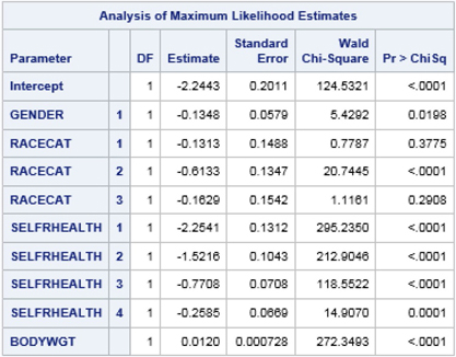
Output 7.2 presents weighted and design-adjusted results for HRS sample-eligible respondents age 50 and older. These results suggest that, holding all other predictors constant, men in the HRS study population are significantly less likely than women to experience diabetes. Respondents who self-report good-to-excellent physical health are significantly less likely than those in poor health to have diabetes. Greater body weight has a significant and positive association with a diagnosis of diabetes. Compared to the other race category (category 4), whites (category 2) are significantly less likely to be diagnosed with diabetes when compared to the other race/ethnicity group. These results will serve as a comparison to results based on the same logistic regression model estimated using multiply imputed data sets (see below).

7.2.3 Multiple Imputation of Missing Data with an Arbitrary Missing Data Pattern Using the FCS Method with Diagnostic Trace Plots

The FCS method is the most flexible procedure for multiply imputing missing data for a mixture of categorical and continuous variables with an arbitrary missing data pattern. In this particular example, use of logistic regression for binary/ordinal variables, the discriminant function for nominal variables, and linear regression for continuous variables is demonstrated.

Highlights of the PROC MI code below include M=3 repetitions, use of a trace plot of estimated means for body weight, NBITER=20 for 20 “burn-in” iterations, and a SEED=55 to ensure the ability to replicate these imputation results. As in previous examples, we use a combined strata/cluster variable and the 2006 respondent weight to enrich the imputation model and reflect the complex sample design characteristics. The use of the CLASS statement instructs PROC MI to treat race, gender, education, self-rated health, diabetes, arthritis, and the combined stratum/SECU variable as classification. For the DISCRIM function imputation, we omit the combined stratum and SECU variable from the imputation model but include it in the logistic and regression imputation models. This is to avoid “stretching the limits” of the DISCRIM function as is designed for use with continuous rather than classification covariates. In this data set, with 56 strata (STRATUM) and values of 1 or 2 in the cluster variable (SECU), adding 56*2=112 predictors to each level of the nominal race/ethnicity outcome would severely test the assumptions of the DISCRIM function and model stability.

proc mi nimpute=3 data=c7_ex1 seed=55 out=c7_ex1_imp;
class racecat gender edcat selfrhealth diabetes arthritis stratum_secu;
fcs plots=trace(mean(bodywgt)) nbiter=20 logistic (edcat diabetes arthritis)
   discrim(racecat=gender edcat selfrhealth diabetes arthritis
   /classeffect=include) regression (bodywgt);
var stratum_secu kwgtr kage gender racecat edcat diabetes arthritis bodywgt
   selfrhealth;
run;

Output 7.3: FCS Variance Information and Parameter Estimates for Body Weight

Output 7.3 includes Variance Information and Parameter Estimates tables with information for just the continuous variable BODYWGT. By default, only continuous variable output is included, and given that the other variables to be imputed are categorical, no descriptive output is automatically generated by PROC MI.

Figure 7.1: Trace Plot for Mean of Body Weight

The Trace Plot (Figure 7.1) includes the mean estimates of body weight for the FCS algorithm at each sequential “burn-in” iteration (iterations 1–20) and the actual imputations 1–3 (iterations 21, 22, and 23). The narrow ranges (about 174.3–174.5 pounds) of the MI repetition mean estimates and absence of systematic trends illustrated in the plot suggest that by the end of the “burn-in” sequence of iterations the FCS imputation algorithm has likely converged to a reasonable predictive distribution for imputation of the missing values of the body weight variable.

7.2.4 Logistic Regression Analysis of Imputed Data Sets Using PROC SURVEYLOGISTIC

Our analytic plan includes use of logistic regression to study the relationship of a diabetes diagnosis with gender, race, self-rated health, and body weight in the HRS population age 50-plus. We now use the imputed data sets from step 1 to perform a design-adjusted logistic regression using PROC SURVEYLOGISTIC with the CLASS, BY, and ODS OUTPUT statements. With the ODS OUTPUT statement, we create a data set of parameter estimates (PARAMETERESTIMATES=) for input into PROC MIANALYZE. Use of the BY _IMPUTATION_ statement produces separate model fit and parameter estimate outputs for each of the three imputation repetition data sets generated by PROC MI.

We recommend a careful check of the contents and structure of the parameter estimate output data sets from PROC SURVEYLOGISTIC to understand the variable naming conventions and how CLASS variable levels are handled. For this task, PROC PRINT is used to list the regression parameter output dataset, c7_ex1_est.

proc surveylogistic data=c7_ex1_imp;
weight kwgtr; strata stratum; cluster secu;
by _imputation_;
class racecat gender edcat selfrhealth / param=ref;
model diabetes (event='1')=gender racecat selfrhealth bodywgt;
ods output parameterestimates=c7_ex1_est;
run;

proc print data=c7_ex1_est;
run ;

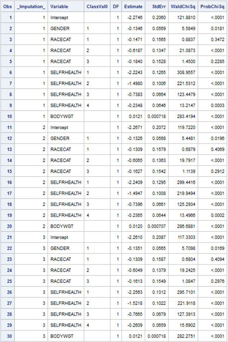
Output 7.4: Listing of Parameter Estimates Output Data Set from PROC SURVEYLOGISTIC

Output 7.4 is a listing of the output estimates data set for the three repetitions from PROC SURVEYLOGISTIC.

7.2.5 Use of PROC MIANALYZE with Logistic Regression Output

We next use PROC MIANALYZE to combine the MI repetition analysis results to generate final MI estimates of parameters and standard errors. A number of options are illustrated, including a CLASS statement, PARMS=(CLASSVAR=CLASSVAL), and EDF=56. The MODELEFFECTS statement uses the information in the VARIABLE and CLASSVAL0 variables (created automatically by SAS with use of the ODS OUTPUT statement above) such that distinct levels of each CLASS variable are recognized. Use of the EDF=56 option ensures that the correct complete complex sample design degrees of freedom for the HRS data are used in significance tests.

proc mianalyze parms(classvar=classval)=c7_ex1_est edf=56;
class racecat gender selfrhealth;
modeleffects intercept gender racecat selfrhealth bodywgt;
run;

Output 7.5: Variance Information and Parameter Estimates from PROC MIANALYZE

Output 7.5 contains Model Information, Variance Information, and the Parameter Estimates table. The Parameter Estimates results suggest that, all else held constant, men (GENDER=1) have significantly lower odds than women of being diagnosed with diabetes; that better self-rated health (SELF_HEALTH=1,2) is associated with lower odds of being diabetic; and that increased body weight has a significant, positive association with diabetes. Comparing individuals by race/ethnicity, Whites (RACECAT=2) have significantly lower odds of diabetes when compared to persons of Other race/ethnicity; however, the odds of diabetes among Hispanic and Black (RACECAT=1,3) adults in the HRS population do not differ significantly from that for Other subpopulation.

7.2.6 Comparison of Complete Case Analysis and Multiply Imputed Analysis

A comparison of the results from complete case analysis (Output 7.2) and MI analysis (Output 7.5) shows little difference between parameter estimates, standard errors, and therefore the nature of the final inferences that we would draw from either approach. In this case, the small difference in results and associated inferences is likely due to relatively low amounts of missing data in the analysis variables. It will not always be true that results from a complete case analysis and a multiple imputation treatment of the data will lead to the same results and inferences. A simple sensitivity test—comparing results of complete case and MI analysis—is a useful tool to help analysts interpret the potential effects (presumably null or positive!) that a correct MI treatment of missing value is having on the analysis and interpretation of their data.

7.3 Imputation and Analysis of Longitudinal Seizure Data

7.3.1 Introduction to the Seizure Data

In our second case study, a data set (c7_ex2) from a study of epileptic seizures is used to demonstrate methods for multiple imputation and analysis of longitudinal/repeated measures data. The data set analyzed in this application consists of counts of the number of seizures experienced in each of four two-week periods during the trial; the baseline number of seizures for the eight-week period prior to the start of the clinical trial; subject ID; age in years; an indicator of whether the subject received an anti-epilepsy drug treatment or placebo (control); and a time variable representing the four two-week periods. For this example, we modified the original data such that there is missing data for one or more of the four seizure count variables. There were 59 unique individuals in the study. For each subject there are four data records, one for each of the four two-week observation periods. The structure of the modified data set is a multiple-records-per-respondent rectangular data array.

The intended analysis focuses on a regression of number of seizures experienced during the trial on the covariates: baseline seizures, age, treatment status, and time (representing the four measurements during the trial). We use a generalized estimating equation (Liang and Zeger 1986) approach with a Poisson model and a repeated statement to account for the lack of independence among two-week seizure counts for each respondent.

Variables used in this analysis are:

ID: Unique numeric id variable, no missing data, 59 unique respondents and 236 person measurements

TIME: A numeric variable ranging from 1–4, corresponding to four two-week periods of the trial, no missing data

AGE: Age in years, numeric variable with no missing data, range is 18–42

TX: Treatment indicator, randomized clinical trial using Progabide, coded 1=Yes, 0=No, no missing data

BASELINE: Number seizures in the baseline eight-week period prior to the start of the trial divided by four to represent seizures per two-week period, numeric, no missing data, range is 1–38 (rounded)

COUNT: Count of seizures experienced during each of four consecutive two-week periods following the eight weeks of pre-trial baseline, numeric, some missing data, range is 0–76

The variables of interest are number of seizures during each two-week period, age, treatment status, and the baseline measurement of seizures. We intend to use a repeated measures Poisson model to regress the count of seizures on age, treatment status, time period of seizure measurements, and baseline number of seizures.

7.3.2 Exploratory Analysis of Seizure Data

After data download, we first explore the variable distributions and missing data patterns in the c7_ex2 data set. This analysis is done once for the full data set and again for the count of seizures during each of four sequential two-week observation periods of the study.

proc means data=c7_ex2 n nmiss mean min max;
var id count baseline age tx time;
run;

proc means data=c7_ex2 n nmiss mean min max;
class time;
var count;
run;

Output 7.6: Exploratory Analysis of Seizure Data

Output 7.6 shows 19 person measurement records with missing data on at least 1 of the 4 seizure counts. For example, the first two-week measurement (TIME=1) has six records missing data, the second measurement has six records without data, the third has two records with missing data, and the fourth has five records with missing data. Given that the data set is structured in a long or multiple records per station format with missing data on some measurements, the ability to account for the dependence within each subject during the imputation is important.

One general method to incorporate the information from multiple records within each person’s data array is to convert the data set from a multiple-records-per-respondent format to a one-record-per-respondent structure with differently named variables for each time point’s measurement. Without restructuring from multiple records per person to one record per person, the relationships within respondents will not be captured in the imputations. Conversion of the data set is recommended for the multiple imputation step, but for subsequent analysis of the imputed data, conversion back to the multiple-records-per-respondent format is recommended (Allison 2001). This approach works well for a variety of missing data problems with some observed data on each of the multiple measurements and a small number of time points or repeated measurements.

We demonstrate the entire process, including data conversion from a multiple- to a single-record structure, multiple imputation of missing values, conversion back to a multiple record data set to analyze imputed data sets, and combining results from the first two MI steps with PROC MIANALYZE.

7.3.3 Conversion of Multiple-Record to Single-Record Data

Each of the 59 respondents has multiple measurement records containing the number of seizures for each period (TIME=1,2,3,4). The listing below contains data records for three respondents. Respondent IDs 101 and 103 have some missing data on the COUNT variable while ID=102 has fully observed data for the variable COUNT.

proc print data=c7_ex2 (obs=12);
run;

Output 7.7: Listing of Seizure Measurements for Three Respondents

Prior to imputation of missing data, the c7_ex2 data set is converted to a one-record-per-individual data set using the SAS code below. We employ array processing in the data step, although PROC TRANSPOSE is another good option. The data set has been previously sorted by ID.

The data step code performs a number of important steps:

1. Produces one record per unique respondent with four variables representing the seizure counts for the four biweekly observation periods (COUNTN1-COUNTN4);

2. Creates an imputation indicator “flag” variable for each of the four count variables (imputation flag variables are named COUNTNI1–COUNTNI4);

3. Outputs the full data vector for each respondent. Because we need one “summary” record for each person, we output only the last record, which contains the full data array.

Note that the last record per respondent contains all of the needed variables and information for the imputation step.

proc sort data=c7_ex2;
by id;
run;

data onerec;
array countn [4];
retain countn1-countn4;
array countni [4];
set c7_ex2;
by id;
countn(time) = count;

do i=1 to 4;
if countn[i] eq . then countni [i]=1; else countni[i]=0;
end;
if last.id then output;
run;

proc print data=onerec (obs=3);
run;

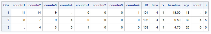
Output 7.8: Listing of One Record per Person Data Format

Output 7.8 lists records for three respondents in the one-record-per-ID format. The output shows that ID=101 has missing data on the fourth measurement (COUNTN4). The next record (ID=102) has fully observed data, and ID=103 is missing a value for the COUNT1 variable only. The COUNTNI1–COUNTNI4 imputation flags are set to one if imputation is needed and zero otherwise.

We now use PROC MI without imputation to examine the missing data pattern. Since a single record has been created for each subject with repeated measures for the time-dependent counts of seizures, we can no longer use the time variable itself in the imputation model. Note that this approach to multiple imputation of the longitudinal missing data does not permit us to fully capture the time-specific ordering of the counts in the imputation model—only the dependencies that exist among the four repeated measures. Each of the other variables used in the imputation are time-invariant and can be used directly in the imputation model.

proc mi nimpute=0 data=onerec;
var tx baseline age countn1-countn4;
run;

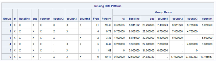
Output 7.9: Missing Data Patterns for Seizure Measurements

Output 7.9 indicates an arbitrary missing data pattern. The seizure count variables have a moderate amount of missing data, with about 30.5% of cases missing on one or more counts. Given the moderately high percentage of missing data on seizure counts, we set the number of imputations to M=10.

7.3.4 Multiple Imputation of Missing Data

With the restructured data set ready for imputation, we use the FCS PMM method to impute the missing data. Highlights of the PROC MI code are: NIMPUTE=10 to produce ten repetition data sets; SEED=45 for potential future replication of the imputation; K=6 option to instruct SAS to use the six closest observed values or “neighbors” for the random draws of a donor value for the missing data imputation.

proc mi nimpute=10 data=onerec seed=45 out=c7_ex2_imp;
var tx baseline age countn1-countn4;
fcs regpmm (countn1-countn4 / k=6);
run ;

Output 7.10: Variance Information and Parameter Estimates

Relative Efficiency of the M=10 imputations is quite high overall (> 0.98 for each imputed variable). The FMI is highest on the first seizure count variable (.1149), reflecting the higher amounts of missing information on the COUNTN1 variable.

With imputation complete, use of PROC MEANS with a CLASS statement allows examination of means for each seizure count variable by _IMPUTATION_ and corresponding imputation flag variable. This set of statements is used within a SAS macro DO loop to reduce the code burden and allow for easy execution of the four cycles of the PROC MEANS analysis.

%macro c (v , iv );
%do i=1 %to 4;
proc means mean min max data=c7_ex2_imp;
var &v.&i;
class &iv.&i;
run;
%end;
%mend;

%c(countn, countni)

Output 7.11: Means for Imputed and Observed Seizure Counts

The imputed versus observed value means illustrate how the overall statistics vary. For example, for the seizure count measurements from time 2, 3 and 4, the means of imputed values are lower than the mean for observed cases. The opposite is true for time 1, where the mean of imputed values exceeds the mean for actual observations (9.91 versus 7.33). These differences are expected and reflect the stochastic nature of the imputations and the associated uncertainty that is inherent in the imputation process—uncertainty that MI also ensures is reflected in estimates and inferences. The minimum and maximum values provide a check of the range of each variable. Note that since the PMM method was used to impute missing values for seizure counts, the minima and maxima never exceed the observed minimum and maximum values of the four seizure count variables. Upon review, these results alone do not signal any apparent problems with the imputation process.

7.3.5 Conversion Back to Multiple Record Data for Analysis of Imputed Data Sets

Prior to further analysis, the data set is returned to a multiple-records-per-respondent structure. Longitudinal data analysis in SAS (typically performed using PROC MIXED, PROC GLIMMIX, PROC NLMIXED, or PROC GENMOD) is generally performed with a “long” or multiple records per unit of analysis data set. Therefore, the process we used for imputation is reversed, again with array processing. Use of a DO loop with an output statement outputs 4 records per respondent, per imputation so our data set now consists of 10 imputations*59 unique people*4 seizure measurements=2,360 records.

The variables ID, TX, BASELINE, AGE, TIME, _IMPUTATION_, and the restructured variables COUNT_IMP and COUNT_IMPF are kept for use in our planned analyses.

data c7_ex2_imp_long
(keep=id tx baseline age time count_imp count_impf_imputation_);
set c7_ex2_imp;
by _imputation_ id;
array mon [4] countn1-countn4;
array imp [4] countni1-countni4;

do i=1 to 4;
count_imp = mon [i];
count_impf= imp [i];
time=i;
output;
end;
run;

proc sort; by _imputation_ id time; run;

proc print data=c7_ex2_imp_long (obs=12);
id _imputation_ id;
run;

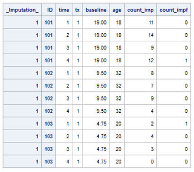
Output 7.12: Listing of First Three Respondents for First Imputation

Output 7.12 highlights the values for IDs 101, 102, and 103 in the first (_Imputation_=1) of the 10 MI repetitions included in the new data set. The TIME variable returns to values of 1 to 4, TX is either 1 or 0 for every record per individual, while the baseline seizure count is repeated 4 times as is the age variable (AGE).

7.3.6 Regression Analysis of Imputed Data Sets

We analyze the imputed data using Poisson regression with the count of seizures regressed on time, treatment status, baseline seizure count, and age. Due to the repeated measurements of seizure counts per individual and inherent dependency among these counts, we use PROC GENMOD with a REPEATED statement. The CLASS statement declares TIME and ID as classification variables. We specify the covariance matrix as autoregressive for one time period (AR=(1)) with LINK=LOG and DIST=POISSON to request Poisson regression. The output data set named c7_ex2_outgenmod is saved via the ODS OUTPUT GEEEMPPEST= statement. Here, the ODS table name corresponds to GEE empirical estimates and robust standard errors by default.

proc genmod data=c7_ex2_imp_long;
by _imputation_ ; class time id;
model count_imp=time age tx baseline / dist=poisson link=log;
repeated subject=id / type=ar(1);
ods output GEEEmpPEst=c7_ex2_out_genmod;
run;
proc print data=c7_ex2_out_genmod;
run;

Output 7.13: Listing of Poisson Regression Estimates by Imputation

Output 7.13 lists the output data set produced by PROC GENMOD (for the first two repetitions only). Note how the parameter estimates and corresponding levels are organized. Because the levels of the TIME variable are contained fully in the LEVEL1 variable, use of the PARMS(CLASSVAR=LEVEL) syntax in PROC MIANALYZE is appropriate.

proc mianalyze parms(classvar=level)=c7_ex2_out_genmod;
class time;
modeleffects intercept time age tx baseline;
run;

Output 7.14: Model, Variance, and Parameter Information for Number of Seizures Model

Based on Output 7.14, age and number of seizures at baseline are positive and significant predictors of seizures during the clinical trial, holding all other covariates constant. Controlling for other factors in the Poisson regression model, neither the trial treatment for epilepsy (TX) nor the time period of observation during the trial results in a significant change in seizure episodes. The variances and standard errors in this analysis are adjusted for both the repeated measures for individuals and the imputation variability through use of the REPEATED statement in PROC GENMOD and the pooled estimates from PROC MIANALYZE.

7.4 Summary

Chapter 7 has illustrated applications of multiple imputation to two case studies. In the first case study, we compare design-adjusted logistic regression results from a complete case analysis with the same design-adjusted logistic regression results from a multiply imputed HRS 2006 data set. The comparison investigates the impact of doing nothing about missing data versus using multiple imputation to deal with missing data problems in a complex sample design data set.

The second case study presents multiple imputation of missing data and subsequent analysis of longitudinal observations on seizures and the impact of treatment during a clinical trial. We present these case studies to provide practical guidance for analysts dealing with similar complex missing data problems in their daily work.

..................Content has been hidden....................

You can't read the all page of ebook, please click here login for view all page.

Table of Contents for Chapter 7: Multiple Imputation Case Studies

Create new playlist

Sign In

Sign Up