11

Introduction to Deep Learning

In the previous chapter, we understood how to use modern machine learning models to tackle time series forecasting. Now, let’s focus our attention on a subfield of machine learning that has shown a lot of promise in the last few years – deep learning. We will be trying to demystify deep learning and go into why it is popular nowadays. We will also break down deep learning into major components and learn about the workhorse behind deep learning – gradient descent.

In this chapter, we will be covering these main topics:

• What is deep learning and why now?
• Components of a deep learning system
• Representation learning
• Linear layers and activation functions
• Gradient descent

Technical requirements

You will need to set up the Anaconda environment following the instructions in the Preface of the book to get a working environment with all the packages and datasets required for the code in this book.

The associated code for the chapter can be found at https://github.com/PacktPublishing/Modern-Time-Series-Forecasting-with-Python-/tree/main/notebooks/Chapter11.

What is deep learning and why now?

In Chapter 5, Time Series Forecasting as Regression, we talked about machine learning and borrowed a definition from Arthur Samuel: “Machine Learning is a field of study that gives computers the ability to learn without being explicitly programmed.” And we further saw how we can learn useful functions from data using machine learning. Deep learning is a subfield of this same field of study. The objective of deep learning is also to learn useful functions from data, but with a few specifications on how it does that.

Before we talk about what is special about deep learning, let’s answer another question first. Why are we talking about this subfield of machine learning as a separate topic? The answer to that lies in the unreasonable effectiveness of deep learning methods in countless applications. Deep learning has taken the world of machine learning by storm, overthrowing state-of-the-art systems across types of data such as images, videos, text, and so on. If you remember the speech recognition systems on phones a decade ago, they were more meme-worthy than really useful. But today, you can say Hey Google, play Pink Floyd and Comfortably Numb will start playing on your phone or speakers. Multiple deep learning systems made this process possible in a smooth way. The voice assistant in your phone, self-driving cars, web search, language translation… the list of applications of deep learning in our day-to-day lives just keeps on going.

By now, you might be wondering what this new technology called deep learning is all about, right? Deep learning is not a new technology. The origins of deep learning can be traced way back to the late 1940s and early 1950s. It only appears to be new because of the recent surge in popularity of the field.

Let’s quickly see why deep learning is suddenly popular.

Why now?

There are two main reasons why deep learning has gained a lot of ground in the last two decades:

• Increase in compute availability
• Increase in data availability

Let’s discuss the preceding points in detail in the following sections.

Increase in compute availability

Back in 1960, Frank Rosenblatt wrote a paper about a three-layer neural network and stated that it went a long way in demonstrating the ability of neural networks as a pattern-recognizing device. But in the same paper, he noted the burden on a digital computer (of the 1960s) was too great as we increase the number of connections. However, in the decades that followed, computer hardware showed close to 50,000 times more improvement, which provided a good boost to neural networks and deep learning. Although it was still not enough as neural networks were still not considered to be good enough for large-scale applications.

This is when a particular type of hardware, which was initially developed for gaming, came to the rescue – GPUs. It’s not entirely clear who started using GPUs for deep learning. Kyoung-Su Oh and Keechul Jung published a paper titled GPU implementation of neural networks back in 2004, which seems to be the first to show massive speed-ups in using GPUs for deep learning. One of the earliest and more popular research papers on the topic came from Rajat Raina, Anand Madhavan, and Andrew Ng, who published a paper titled Large-scale deep unsupervised learning using graphics processors back in 2009. It showed the effectiveness of GPUs for deep learning.

Although many groups led by LeCun, Schmidhuber, Bengio, and so on were playing around with using GPUs, the turning point really came when Alex Krizhevsky, Ilya Sutskever, and Geoffrey E. Hinton used a GPU-based deep learning system that outperformed all the other competing technologies in an image recognition contest called the ImageNet Large Scale Visual Recognition Challenge 2012. The introduction of GPUs provided the much-needed boost to the widespread use of deep learning and accelerated the progress in the field.

Reference check

The research papers GPU implementation of neural networks, Large-scale deep unsupervised learning using graphics processors, and ImageNet Classification with Deep Convolutional Neural Networks are cited in the References section under 1, 2, and 3, respectively.

Increase in data availability

In addition to the skyrocketing compute capability, the other main factor that helped deep learning is the sheer increase in data. As the world became more and more digitized, the amount of data that we generate increased drastically. Tables that had hundreds and thousands of rows now exploded into millions and billions of rows, and the ever-decreasing cost of storage helped this explosion of data collection.

And why would an increase in data availability help deep learning? This lies in the way deep learning works. Deep learning is quite data-hungry and needs large amounts of data to learn good models. Therefore, if we keep increasing the data that we provide to a deep learning model, the model will be able to learn better and better functions. But the same can’t be said for the traditional machine learning models. Let’s cement this learning with a chart that Andrew Ng, a world-renowned ML educator and an adjunct professor at Stanford, popularized in his famous machine learning course – Machine Learning by Stanford University in Coursera (Figure 11.1).

Figure 11.1 – Deep learning versus traditional machine learning as we increase the data size

In Figure 11.1, which was popularized by Andrew Ng, we can see that as we increase the data size, traditional machine learning hits a plateau and won’t improve anymore.

It has been proven empirically that there are significant benefits to the overparameterization of a deep learning model. Overparameterization means that there are more parameters in the model than the number of data points available to train. In classical statistics, this is a big no-no because, under this scenario, the model invariably overfits. But deep learning seems to flaunt this rule with ease. One of the examples of overparameterization is the current state-of-the-art image recognition system, NoisyStudent. It has 480 million parameters, but it was trained on ImageNet with 1.2 million data points.

It has been argued that the way deep learning models are trained (stochastic gradient descent, which we will be explaining soon) is the key because it has a regularizing effect. In a research paper titled The Computational Limits of Deep Learning, Niel C. Thompson and others tried to illustrate this using a simple experiment. They set up a dataset with 1,000 features, but only 10 of them had any signal in them. Then they tried to learn four models based on the dataset using varying dataset sizes:

• Oracle model – A model that uses the exact 10 parameters that have any signal in them.
• Expert model – A model that uses 9 out of 10 significant parameters.
• Flexible model – A model that uses all 1,000 parameters.
• Regularized model – A model that uses all 1,000 parameters, but is now a regularized (lasso) model. (We covered regularization back in Chapter 8, Forecasting Time Series with Machine Learning Models.)

Let’s see Figure 11.2 from the research paper with the study:

Figure 11.2 – The chart shows how different models perform under different sizes of data

The chart has a number of data points used on the x axis, and the performance (-log(Mean Squared Error)) on the y axis. The different colored lines show the different types of models. The regularized model (which is a proxy for deep learning models) keeps improving as we give the model more and more data, whereas the expert model (a proxy for machine learning model) plateaus. This strengthens the concept Andrew Ng popularized once more – with more data, deep learning starts to outperform traditional machine learning.

A lot more factors, apart from compute and data availability, have contributed to the success of deep learning. Sara Hooker, in her essay The Hardware Lottery (#9 in References), talks about how an idea wins not necessarily because it is superior to other ideas, but because it is suited to the software and hardware available at the time. And once a research direction gets the lottery, it snowballs because more funding and big research organizations get behind that idea and it eventually becomes the most prominent idea in the space of ideas.

We have talked about deep learning for some time but have still not understood what it is. Let’s do that now.

What is deep learning?

There is no single definition of deep learning because it means slightly different things to different people. However, a large majority of people agree on one thing: a model is called deep learning when it involves automatic feature learning from raw data. As Yoshua Bengio (a Turing Award winner and one of the godfathers of AI) explains it in his 2021 paper titled Deep Learning of Representations for Unsupervised and Transfer Learning:

“Deep learning algorithms seek to exploit the unknown structure in the input distribution in order to discover good representations, often at multiple levels, with higher-level learned features defined in terms of lower-level features.”

Peter Norvig, the Director of Research at Google, has a similar but simpler definition:

“A kind of learning where the representation you form have (sic) several levels of abstraction, rather than a direct input to output.”

Another key feature of deep learning a lot of people agree upon is compositionality. Yann LeCun, a Turing Award winner and another one of the godfathers of AI, has a slightly more complex, but more exact definition of deep learning:

“DL is methodology: building a model by assembling parameterized modules into (possibly dynamic) graphs and optimizing it with gradient-based methods.”

The key points we would like to highlight here are as follows:

• Assembling parametrized modules – This refers to the compositionality of deep learning. Deep learning systems, as we will shortly see, are composed of a few submodules with a few parameters (some without) assembled into a graph-like structure.
• Optimizing it with gradient-based methods – Although having gradient-based learning as a sufficient criterion for deep learning is not widely accepted, we can still see empirically that, today, most successful deep learning systems are trained using gradient-based methods. (If you are not aware of what a gradient-based optimization method is, don’t worry. We will be covering it soon in this chapter.)

If you have read anything about deep learning before, you may have seen neural networks and deep learning used together, or interchangeably. But we haven’t talked about neural networks till now. Before we do that, let’s look at a fundamental unit of any neural network.

Perceptron – the first neural network

A lot of what we call deep learning and neural networks are deeply influenced by the human brain and its inner workings. The human desire to create intelligent beings like themselves was manifested as early as back in Greek mythology (Galatea and Pandora). And owing to this desire, humans have studied and looked for inspiration from human anatomy for years. One of the organs of the human body that has been studied intensely is the brain because it is the center of intelligence, creativity, and everything else that makes a human.

Even though we still don’t know a lot about the brain, we do know a bit about it, and we use that little information to design artificial systems. The fundamental unit of a human brain is something we call a neuron, shown here:

Figure 11.3 – A biological neuron

Many of you might have come across this in biology or in the context of machine learning as well. But let’s refresh this anyway. The biological neuron has the following parts:

• Dendrites are branched extensions of the nerve cell that collect inputs from surrounding cells or other neurons.
• Soma, or the cell body, collects these inputs, joins them, and is passed on.
• Axon hillock connects the soma to the axon, and it controls the firing of the neuron. If the strength of a signal exceeds a threshold, the axon hillock fires an electrical signal through the axon.
• Axon is the fiber that connects the soma to the nerve endings. It is the axon’s duty to pass on the electrical signal to the endpoints.
• Synapses are the end points of the nerve cell and transmit the signal to other nerve cells.

McCulloch and Pitts (1943) were the first to design a mathematical model for the biological neuron. But the McCulloch-Pitts model had a few limitations:

• It only accepted binary variables.
• It considered all input variables equally important.
• There was only one parameter, a threshold, which was not learnable.

In 1957, Frank Rosenblatt generalized the McCulloch-Pitts model and made it a full model whose parameters could be learned.

Reference check

The original research paper for Frank Rosenblatt’s Perceptron is cited in References under reference number 5.

Let’s understand the Perceptron in detail because it is the fundamental building block of all neural networks:

Figure 11.4 – Perceptron

As we see from Figure 11.4, the Perceptron has the following components:

• Inputs – These are the real-valued inputs that are fed to a Perceptron. This is like the dendrites in neurons that collect the input.
• Weighted sum – Each input is multiplied by a corresponding weight and summed up. The weights determine the importance of each input in determining the outcome.
• Non-linearity – The weighted sum goes through a non-linear function. For the original Perceptron, it was a step function with a threshold activation. The output would be positive or negative based on the weighted sum and the threshold of the unit. Modern-day Perceptrons and neural networks use different kinds of activation functions, but we will see that later on.

We can write the Perceptron in the mathematical form as follows:

Figure 11.5 – Perceptron – a math perspective

As shown in Figure 11.5, the Perceptron output is defined by the weighted sum of inputs, which is passed in through a non-linear function. Now, we can think of this using linear algebra as well. This is an important perspective for two reasons:

• The linear algebra perspective will help you understand neural networks faster.
• It will also make the whole thing feasible because matrix multiplications are something that our modern-day computers and GPUs are really good at. Without linear algebra, multiplying these inputs with corresponding weights would require us to loop through the inputs, and it quickly becomes infeasible.

Linear algebra intuition recap

Let’s take a look at a couple of concepts as a refresher.

Vectors and vector spaces

At the superficial level, a vector is an array of numbers. But in linear algebra, a vector is an entity that has both magnitude and direction. Let’s take an example to elucidate:

We can see that this is an array of numbers. But if we plot this point in the two-dimensional coordinate space, we get a point. And if we draw a line from the origin to this point, we will get an entity with direction and magnitude. This is a vector.

The two-dimensional coordinate space is called a vector space. A two-dimensional vector space, informally, is all the possible vectors with two entries. And extending it to n-dimensions, an n-dimensional vector space is all the possible vectors with n entries.

The final intuition I want to leave with you is this: a vector is a point in the n-dimensional vector space.

Matrices and transformations

Again, at the superficial level, a matrix is a rectangular arrangement of numbers that looks like this:

Matrices have many uses but the one intuition that is most relevant for us is that a matrix specifies a linear transformation of the vector space it resides in. When we multiply a vector with a matrix, we are essentially transforming the vector, and the values and dimensions of the matrix define the kind of transformation that happens. Depending on the content of the matrix, it does rotation, reflection, scaling, shearing, and so on.

We have included a notebook in the chapter11 folder titled 01-Linear Algebra Intuition.ipynb, which explores matrix multiplication as a transformation. We also apply these transformation matrices to vector spaces to develop intuition on how matrix multiplication can rotate and warp the vector spaces.

I highly suggest heading over to the Further reading section where we have given a few resources to get started and solidify necessary intuition.

If we consider the inputs as vectors in the feature space (vector space with m-dimensions), the term is nothing but a linear combination of input vectors. We can convert this to vector dot products by . We can include the bias also in there by adding an additional dummy input with a fixed value of 1 and adding to the vector. This is what is shown in Figure 11.5 as the vector representation.

Now that we have had an introduction to deep learning, let us recall one of the aspects of deep learning we discussed earlier – compositionality – and explore it a bit more deeply in the next section.

Components of a deep learning system

Let us recall Yann LeCun’s definition of deep learning:

“Deep learning is a methodology: building a model by assembling parameterized modules into (possibly dynamic) graphs and optimizing it with gradient-based methods.”

The core idea here is that deep learning is an extremely modular system. Deep learning is not just one model, but rather a language to express any model in terms of a few parametrized modules with these specific properties:

• It should be able to produce an output from a given input through a series of computations.
• If the desired output is given, they should be able to pass on information to its inputs on how to change, to arrive at the desired output. For instance, if the output is lower than what is desired, the module should be able to tell its inputs to change in some direction so that the output becomes closer to the desired one.

The more mathematically inclined may have figured out the connection to the second point of differentiation. And you would be correct. To optimize these kinds of systems, we predominantly use gradient-based optimization methods. Therefore, condensing the two properties into one, we can say that these parameterized modules should be differentiable functions.

Let’s take the help of a visual to aid further discussion:

Figure 11.6 – A deep learning system

As shown in Figure 11.6, deep learning can be thought of as a system that takes in raw input data through a series of linear and non-linear transforms to provide us with an output. It also can adjust its internal parameters to make the output as close as possible to the desired output through learning. To make the diagram simpler, we have chosen a paradigm that fits most of the popular deep learning systems. It all starts with raw input data. The raw input data goes through N blocks of linear and non-linear functions that do representation learning. Let’s explore this block in some detail.

Representation learning

Representation learning, informally, learns the best features by which we can make the problem linearly separable. Linearly separable means when we can separate the different classes (in a classification problem) with a straight line (Figure 11.7):

Figure 11.7 – Transforming non-linearly separable data into linearly separable using a function,

The representation learning block in Figure 11.6 may have multiple linear and non-linear functions stacked on top of each other and the overall function of the block is to learn a function, , which transforms the raw input into good features that make the problem linearly separable.

Another way to look at this is through the lens of linear algebra. As we explored earlier in the chapter, matrix multiplication can be thought of as a linear transformation of vectors. And if we extend that intuition to the vector spaces, we can see that matrix multiplication warps the vector space in some way or another. And when we stack multiple linear and non-linear transformations on top of each other, we are essentially warping, twisting, and squeezing the input vector space (with the features) into another space. When we are asking a parameterized system to warp the input space (pixels of images) in such a way as to perform a particular task (such as the classification of dogs versus cats), the representation learning block learns the right transformations, which makes the task (separating cats from dogs) easier.

I have created a video illustrating this because nothing establishes an intuition better than a video of what is happening. I’ve taken a sample dataset that is not linearly separable, trained a neural network on the problem to classify, and then visualized how the input space was transformed by the model into a linearly separable representation. You can find the video here: https://www.youtube.com/watch?v=5xYEa9PPDTE.

Now, let’s look inside the representation learning block. We can see there is a linear transformation and a non-linear activation.

Linear transformation

Linear transformations are just transformations that are applied to the vector space. When we say linear transformation in a neural network context, we actually mean affine transformations.

A linear transformation fixes the origin while applying the transformation, but an affine transformation doesn’t. Rotation, reflection, scaling, and so on are purely linear transformations because the origin won’t change while we do this. But something like a translation, which moves the vector space, is an affine transformation. Therefore is a linear transformation, but is an affine transformation.

So, linear transformations are simply matrix multiplications that transform the input vector space, and this is at the heart of any neural network or deep learning system today.

What happens if we stack linear transformations on top of each other? For instance, we first multiply the input, X, with a transformation matrix, A, and then multiply the results with another transformation matrix, B:

By the associative property (which is applicable for linear algebra as well), we can rewrite this equation as follows:

Generalizing this to a stack of N transformation matrices, we can see that it all works out to be a single linear transformation. This kind of defeats the purpose of stacking N layers, doesn’t it?

This is where the non-linearity becomes essential and we introduce non-linearities by using a non-linear function, which we call activation functions.

Activation functions

Activation functions are non-linear differentiable functions. In a biological neuron, the axon hillock decides whether to fire a signal based on the inputs. The activation functions serve a similar function and are key to the neural network’s ability to model non-linear data. Or in other words, activation functions are key in neural networks’ ability to transform input vector space (which is linearly inseparable) to a linearly separable vector space, informally. To unwarp a space such that linearly inseparable points become linearly separable, we need to have non-linear transformations.

We repeated the same experiment we did in the last section, where we visualized the trained transformation of a neural network on the input vector space, but this time without any non-linearities. The resulting video can be found here: https://www.youtube.com/watch?v=z-nV8oBpH2w. The best transformation that the model learned is just not sufficient and the points are still linearly inseparable.

Theoretically, an activation function can be any non-linear differentiable (differentiable almost everywhere, to be exact) function. But over the course of time, there are a few non-linear functions that are popularly used as activation functions. Let’s look at a few of them.

Sigmoid

Sigmoid is one of the most common activation functions around, and probably one of the oldest. It is also known as the logistic function. When we discussed Perceptron, we mentioned a step (also called heavyside in literature) function as the activation function. The step function is not a continuous function and hence is not differentiable everywhere. A very close substitute is the sigmoid function.

It is defined as follows:

Sigmoid is a continuous function and therefore is differentiable everywhere. The derivative is also computationally simpler to calculate. Because of these properties of the sigmoid, it was adopted widely in the early days of deep learning as a standard activation function.

Let’s see what a sigmoid function looks like and how it transforms a vector space:

Figure 11.8 – Sigmoid activation function (left) and original, and activated vector space (middle and right)

The sigmoid function squashes the input between 0 and 1 as seen in Figure 11.8 (left). We can observe the same phenomenon in the vector space. One of the drawbacks of the sigmoid function is that the gradients tend to zero on the flat portions of the sigmoid. When a neuron approaches this area in the function, the gradients that it receives and propagates become negligible and the unit stops learning. We call this saturating of the activation. Because of this, nowadays, sigmoid is not typically used in deep learning, except in the output layer (we will be talking about this usage soon).

Hyperbolic tangent (tanh)

Hyperbolic tangents are another popular activation. They can be easily defined as follows:

It is very similar to sigmoid. In fact, we can express tanh as a function of sigmoid. Let’s see what the activation function looks like:

Figure 11.9 – TanH activation function (left) and original, and activated vector space (middle and right)

We can see that the shape is similar to sigmoid, although a bit sharper. But the key difference is that the tanh function outputs a value between -1 and 1. And because of the sharpness, we can also see the vector space getting pushed out to the edges as well. The fact that the function outputs a value that is symmetrical around the origin (0) works well with the optimization of the network and hence tanh was preferred over sigmoid. But since the tanh function is also a saturating function, the same problem of very small gradients hampering the flow of gradients and, in turn, learning plagues tanh activations as well.

Rectified linear unit and variants

As neuroscience gained more information about the human brain, researchers found out that only one to four percent of neurons in the brain are activated at any time. But with all the activation functions such as sigmoid or tanh, almost half of the neurons in a network are activated. In 2010, Vinod Nair and Geoffrey Hinton proposed rectified linear units (ReLUs) in the seminal paper Rectified Linear Units Improve Restricted Boltzmann Machines. And ever since, ReLUs have taken over as the de facto activation functions for deep neural networks.

ReLU

A ReLU is defined as follows:

It is just a linear function, but with a kink at zero. Any value greater than zero is retained as is, but all values below zero are squashed to zero. The range of the output goes from 0 to . Let’s see how it looks visually:

Figure 11.10 – ReLU activation function (left) and original, and activated vector space (middle and right)

We can see that the points in the left and bottom quadrants are all pushed into the axes' lines. This squashing is what gives the non-linearity to the activation function. And because of the way the activation sharply becomes zero and does not tend to zero like the sigmoid or tanh, ReLUs are non-saturating.

Reference check

The research paper that proposed ReLU is cited in References under reference number 7.

There are a lot of advantages to using ReLUs:

• The computations of the activation function as well as its gradients are really cheap.
• Training converges much faster than those with saturating activation functions.
• ReLU helps bring sparsity in the network (by having the activation as zero, a large majority of neurons in the network can be turned off) and resembles how biological neurons work.

But ReLUs are not without problems:

• When , the gradients become zero. This means a neuron that has an output < 0 will have zero gradients and therefore, the unit will not learn anymore. These are called dead ReLUs.
• Another disadvantage is that the average output of a ReLU unit is positive and when we stack multiple layers, this might lead to a positive bias in the output.

Let’s see a few variants that tried to resolve the problems we discussed for ReLU.

Leaky ReLU and parametrized ReLU

Leaky ReLU is a variant of standard ReLU that resolves the dead ReLU problem. It was proposed by Maas and others in 2013. A Leaky ReLU can be defined as follows:

Here, is the slope parameter (typically set to a very small value such as 0.001) and is considered a hyperparameter. This makes sure the gradients are not zero when x<0 and thereby ensures there are no dead ReLUs. But the sparsity that ReLU provides is lost here because there is no zero output that turns off a unit completely. Let’s visualize this activation function:

Figure 10.11 – Leaky ReLU activation function (left) and original, and activated vector space (middle and right)

In 2015, He and others proposed another minor modification to Leaky ReLU called parametrized ReLU. In parametrized ReLU, instead of considering as a hyperparameter, they considered it as a learnable parameter.

Reference check

The research paper that proposed leaky ReLU is cited in References under reference number 8, and parametrized ReLU is cited under reference number 9.

There are many other activation functions that are less popularly used but still have enough use cases to be included in PyTorch. You can find a list of them here: https://pytorch.org/docs/stable/nn.html#non-linear-activations-weighted-sum-nonlinearity. We encourage you to use the notebook titled 02-Activation Functions.ipynb in the Chapter 11 folder to try out different activation functions and see how they warp the vector space.

And with that, we now have an idea of the components of the first block in Figure 11.6, representation learning. The next block in there is the linear classifier, which has a linear transformation and an output activation. We already know what a linear transformation is, but what is an output activation?

Output activation functions

Output activation functions are functions that enforce a few desirable properties to the output of the network.

Additional reading

These functions have a deeper connection with maximum likelihood estimation (MLE) and the chosen loss function, but we will not be getting into that because it is out of the scope of this book. We have linked to the book Deep Learning by Ian Goodfellow, Yoshua Bengio, and Aaron Courville in the Further reading section. If you are interested in a deeper understanding of deep learning, we suggest you use the book to that effect.

If we want the neural network to predict a continuous number in the case of regression, we just use a linear activation function (which is like saying there is no activation function). The raw output from the network is considered the prediction and fed into the loss function.

But in the case of classification, the desired output is a class out of all possible classes. If there are only two classes, we can use our old friend, the sigmoid function, which has an output between 0 and 1. We can also use tanh because its output is going to be between -1 and 1. The sigmoid function is preferred because of the intuitive probabilistic interpretation that comes along with it. The closer the value is to one, the more confident the network is about that prediction.

Now, sigmoid works for binary classification. What about multiclass classification where the possible classes are more than two?

Softmax

Softmax is a function that converts a vector of K real values into another K-positive real value, which sums up to one. Softmax is defined as follows:

This function converts the raw output from a network into something that resembles a probability across K classes. This has a strong relation with sigmoid – sigmoid is a special case of softmax when K=2. In the following figure, let’s see how a random vector of size 3 is converted into probabilities that add up to one:

Figure 11.12 – Raw output versus softmax output

If we look closely, we can see that in addition to converting the real values into something that resembles probability, it also increases the relative gap between the maximum and the rest of the values. This activation is a standard output activation for multiclass classification problems.

Now, there is only one major component left in the diagram (Figure 11.6) – the loss function.

Loss function

The loss function we touched upon in Chapter 5, Time Series Forecasting as Regression, translates nicely to deep learning. In deep learning also, the loss function is a way to tell how good the predictions of the model are. If the predictions are way off the target, the loss function would be higher and as we get closer to the truth, it becomes smaller. In the deep learning paradigm, we just have one more additional requirement from the loss function – it should be differentiable.

Common loss functions from classical machine learning, such as mean squared error or mean absolute error, are valid in deep learning as well. In fact, in regression tasks, they are the default choices that practitioners adopt. For classification tasks, we adopt a concept borrowed from information theory called cross-entropy loss. But since deep learning is a very flexible framework, we can use any loss function as long as it is differentiable. There are a lot of loss functions people have already tried and found working in many situations. A lot of them are part of PyTorch’s API as well. You can find them here: https://pytorch.org/docs/stable/nn.html#loss-functions.

Now that we have covered all the components of a deep learning system, let’s also briefly look at how we train the whole system.

Forward and backward propagation

In Figure 11.6, we can see two sets of arrows, one going toward the desired output from input, marked as Forward Computation, and another going backward to the input from the desired output, marked Backward Computation. These two steps are at the core of learning a deep learning system. In the Forward Computation, popularly known as Forward Propagation, we use the series of computations that are defined in the layers and propagate the input all the way through the network to get the output. And now that we have the output, we would use the loss function to assess how close or far we are from the desired output. This information is now used in the Backward Computation, popularly known as Backward Propagation, to calculate the gradient with respect to all the parameters.

Now, what is a gradient and why do we need it? In high school math, we might have come across gradients or derivatives in another form called slope. It is the rate of change of a quantity when we change a variable by unit measure. Derivatives inform us of the local slope of a scalar function. While derivatives are always with respect to a single variable, gradients are a generalization of derivatives to multivariate functions. Intuitively, both gradient and derivatives inform us of the local slope of the function. And with the gradient of the loss function, we can use one of the techniques from mathematical optimization called gradient descent, to optimize our loss function.

Let’s see this with an example.

Gradient descent

Any machine learning or deep learning model can be thought of as a function that converts an input, x, to an output, using a few parameters, . Here, can be the collection of all the matrix transformations that we do to the input throughout the network. But to simplify the example, let’s assume there are only two parameters, a and b. And if we think about the whole process of learning a bit, we will see that by keeping the input and expected output the same, the way to change your loss would be by changing the parameters of the model. Therefore, we can postulate the loss function to be parameterized by the parameters, in this case, a and b.

Notebook alert

To follow along with the complete code, use the notebook named 03-Gradient Descent.ipynb in the chapter11 folder and the code in the src folder.

Let’s assume the loss function takes the following form:

Let’s see what the function looks like. We can use a three-dimensional plot to visualize a function with two parameters, as seen in Figure 11.13. Two dimensions will be used to denote the two parameters and at each point in that two-dimensional mesh, we can plot the loss value in the third dimension. This kind of plot of the loss function is also called a loss curve (in univariate settings), or loss surface (in multivariate settings).

Figure 11.13 – Loss surface plot

The lighter portion of the 3D shape is where the loss function is less and as we move away from there, it increases.

In machine learning, our aim is to minimize the loss function, or in other words, find the parameters that make our predicted output as close as possible to the ground truth. This falls under the realm of mathematical optimization and a particular technique lends itself suitable for this approach – gradient descent.

Gradient descent is a mathematical optimization algorithm used to minimize a cost function by iteratively moving in the direction of the steepest descent. In a univariate function, the derivative (or the slope) gives us the direction (and magnitude) of the steepest ascent. For instance, if we know that the slope of a function is 1, we know if we move to the right, we are climbing up the slope, and moving to the left, we will be climbing down. Similarly, in the multivariate setting, the gradient of a function at any point will give us the direction (and magnitude) of the steepest ascent. And since we are concerned with minimizing a loss function, we will be using the negative gradient, which will point us in the direction of the steepest descent.

So, let’s define the gradient for our loss function. We are using high school calculus, but even if you are not comfortable, you don’t need to worry:

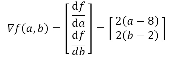
Now, how does the algorithm work? Very simply, as follows:

1. Initialize the parameters to random values.
2. Compute the gradient at that point.
3. Make a step in the direction opposite to the gradient.
4. Repeat steps 2 and 3 until it converges, or we reach maximum iterations.

There is just one more aspect that needs more clarity: how much of a step do we take in each iteration?

Ideally, the magnitude of the gradient tells you how fast the function is changing in that direction, and we should just take the step equal to the gradient. But there is a property of the gradient that makes that a bad idea. The gradient only defines the direction and magnitude of the steepest ascent in the infinitesimally small locality of the current point and is blind to what happens beyond it. Therefore, we use a hyperparameter, commonly called the learning rate, to temper the steps we take in each iteration. Therefore, instead of taking a step equal to the gradient, we take a step equal to the learning rate multiplied by the gradient.

Mathematically, if is the vector of parameters, at each iteration, we update the parameters using the following formula:

Here, is the learning rate and is the gradient at the point.

Let’s see a very simple implementation of gradient descent. First, let’s define a function that returns us the gradient at any point:

def gradient(a, b):
    return 2*(a-8), 2*(b-2)

Now we define a few initial parameters such as the maximum iterations, learning rate, and initial value of a and b:

# maximum number of iterations that can be done
maximum_iterations = 500
# current iteration
current_iteration = 0
# Learning Rate
learning_rate = 0.01
#Initial value of a, b
current_a_value = 28
current_b_value = 27

Now all that is left is the actual process of gradient descent:

while current_iteration < maximum_iterations:
    previous_a_value = current_a_value
    previous_b_value = current_b_value
    # Calculating the gradients at current values
    gradient_a, gradient_b = gradient(previous_a_value, previous_b_value)
    # Adjusting the parameters using the gradients
    current_a_value = current_a_value - learning_rate * gradient_a * (previous_a_value)
    current_b_value = current_b_value - learning_rate * gradient_b * (previous_b_value)
    current_iteration = current_iteration + 1

We know the minimum for this function will be at a=8 and b=2 because that would make the loss function zero. And gradient descent finds a solution that is pretty accurate – a = 8.000000000000005 and b = 2.000000002230101. We can also visualize the path it took to reach the minimum, as seen in Figure 11.14:

Figure 11.14 – Gradient descent optimization on the loss surface

We can see that even though we initialized the parameters far from the actual origin, the optimization algorithm makes a direct path to the optimal point. At each point, the algorithm looks at the gradient of the point and moves in the opposite direction, and eventually converges on the optimum.

When gradient descent is adopted in a learning task, there are a few kinks to be noted. Let’s say we have a dataset of N samples. There are three popular variants of gradient descent that are used in learning and each of them has its pros and cons.

Batch gradient descent

We run all N samples through the network and average the losses across all N instances. Now, we use this loss to calculate the gradient and make a step in the right direction and repeat.

The pros are as follows:

• The optimization path is direct, and it has guaranteed convergence.

The cons are as follows:

• The entire dataset needs to be evaluated for a single step and that is computationally expensive. The computation per optimization step becomes prohibitively high for huge datasets.
• The time taken per optimization step is high and hence the convergence will also be slow.

Stochastic gradient descent (SGD)

In SGD, we randomly sample one instance from N samples, calculate the loss and gradients, and then make an update to the parameters.

The pros are as follows:

• Since we only use a single instance to make the optimization step, computation per optimization step is very low.
• Time taken per optimization step is also faster.
• Stochastic sampling also acts as regularization and helps to avoid overfitting.

The cons are as follows:

• The gradient estimates are noisy because we are making the step based on just one instance. Therefore, the path toward optimum will be choppy and noisy.
• Just because the time taken per optimization is low, it need not mean convergence is faster. We may not be taking the right step many times because of noisy gradient estimates.

Mini-batch gradient descent

Mini-batch gradient descent is a technique that falls somewhere between the spectrum of batch gradient descent and SGD. In this variant, we have another quality called mini-batch size (or simply batch size), b. And in each optimization step, we randomly pick b instances from N samples and calculate gradients on the average loss of all b instances. With b = N, we have batch gradient descent, and with b = 1, we have stochastic gradient descent. This is the most popular way neural networks are trained today. By varying the batch size, we can travel between the two variants and manage the pros and cons of each option.

Nothing develops intuition better than a visual playground where we can see the effects of the different components we discussed. Tensorflow Playground is an excellent resource (see the link in the Further reading section) to do just that. I strongly urge you to head over there and play with the tool, train a few neural networks right in the browser, and see in real time how the learning happens.

Summary

We kicked off a new section of the book with an introduction to deep learning. We started with a bit of history to understand why deep learning is so popular today and we also explored its humble beginnings in Perceptron. We understood the composability of deep learning and understood and dissected the different components of deep learning such as the representation learning block, linear layers, activation functions, and so on. Finally, we rounded off the discussion by looking at how a deep learning system uses gradient descent to learn from data. With that understanding, we are now ready to move on to the next chapter, where we will drive the narrative toward time series models.

References

Following is the list of the reference used throughout this chapter:

1. Kyoung-Su Oh and Keechul Jung. (2004), GPU implementation of neural networks. Pattern Recognition, Volume 37, Issue 6, 2004: https://doi.org/10.1016/j.patcog.2004.01.013.
2. Rajat Raina, Anand Madhavan, and Andrew Y. Ng. (2009), Large-scale deep unsupervised learning using graphics processors. In Proceedings of the 26th Annual International Conference on Machine Learning (ICML ‘09): https://doi.org/10.1145/1553374.1553486.
3. Alex Krizhevsky, Ilya Sutskever, and Geoffrey E. Hinton. (2012), ImageNet Classification with Deep Convolutional Neural Networks. Commun. ACM 60, 6 (June 2017), 84–90: https://doi.org/10.1145/3065386.
4. Neil C. Thompson, Kristjan Greenewald, Keeheon Lee, and Gabriel F. Manso. (2020). The Computational Limits of Deep Learning. arXiv:2007.05558v1 [cs.LG]: https://arxiv.org/abs/2007.05558v1.
5. Frank Rosenblatt. (1957), The perceptron – A perceiving and recognizing automaton, Technical Report 85-460-1, Cornell Aeronautical Laboratory.
6. Charu C. Aggarwal, Alexander Hinneburg, and Daniel A. Keim. (2001). On the Surprising Behavior of Distance Metrics in High Dimensional Spaces. In Proceedings of the 8th International Conference on Database Theory (ICDT ‘01). Springer-Verlag, Berlin, Heidelberg, 420–434: https://dl.acm.org/doi/10.5555/645504.656414.
7. Nair, V., and Hinton, G.E. (2010). Rectified Linear Units Improve Restricted Boltzmann Machines. ICML: https://icml.cc/Conferences/2010/papers/432.pdf.
8. Andrew L. Maas and Awni Y. Hannun and Andrew Y. Ng. (2013). Rectifier nonlinearities improve neural network acoustic models. ICML Workshop on Deep Learning for Audio, Speech, and Language Processing: https://ai.stanford.edu/~amaas/papers/relu_hybrid_icml2013_final.pdf.
9. He, K., Zhang, X., Ren, S., and Sun, J. (2015). Delving Deep into Rectifiers: Surpassing Human-Level Performance on ImageNet Classification. 2015 IEEE International Conference on Computer Vision (ICCV), 1026-1034: https://ieeexplore.ieee.org/document/741048.0
10. Sara Hooker. (2021). The hardware lottery. Commun. ACM, Volume 64: https://doi.org/10.1145/3467017.

Further reading

You can check out the following sources if you want to read more about a few topics covered in this chapter:

• Linear Algebra course from Gilbert Strang: https://ocw.mit.edu/resources/res-18-010-a-2020-vision-of-linear-algebra-spring-2020/videos/
• Essence of Linear Algebra from 3Blue1Brown: https://www.youtube.com/playlist?list=PLZHQObOWTQDPD3MizzM2xVFitgF8hE_ab
• Neural Networks – A Linear Algebra Perspective by Manu Joseph: https://deep-and-shallow.com/2022/01/15/neural-networks-a-linear-algebra-perspective/
• Deep Learning – Ian Goodfellow, Yoshua Bengio, Aaron Courville: https://deep-and-shallow.com/2022/01/15/neural-networks-a-linear-algebra-perspective/
• Tensorflow Playground: https://playground.tensorflow.org/