5

Time Series Forecasting as Regression

In the previous part of the book, we have developed a fundamental understanding of time series and equipped ourselves with tools and techniques to analyze and visualize time series and even generate our first baseline forecasts. We have mainly covered classical and statistical techniques in this book so far. Let’s now dip our toes into modern machine learning and learn how we can leverage this comparatively newer field for time series forecasting. Machine learning is a field that has grown in leaps and bounds in recent times, and being able to leverage these newer techniques for time series forecasting is a skill that will be invaluable in today’s world.

In this chapter, we will be covering these main topics:

• Understanding the basics of machine learning
• Time series forecasting as regression
• Local versus global models

Understanding the basics of machine learning

Before we get started with using machine learning for time series, let’s spend some time establishing what machine learning is and setting up a framework to demonstrate what it does (if you are already very comfortable with machine learning, feel free to skip ahead, or just stay with us and refresh the concepts). In 1959, Arthur Samuel defined machine learning as a “field of study that gives computers the ability to learn without being explicitly programmed.” Traditionally, programming has been a paradigm under which we know a set of rules/logic to perform an action, and that action is performed on the given data to get the output that we want. But, machine learning flipped this on its head. In machine learning, we start with data and the output, and we ask the computer to tell us about the rules with which the desired output can be achieved from the data:

Figure 5.1 – Traditional programming versus machine learning

There are many kinds of problem settings in machine learning, such as supervised learning, unsupervised learning, self-supervised learning, and so on, but we will stick to supervised learning, which is the most popular one and the most applicable one to the contents of this book.

Let’s start our discussion small and slowly build up to the whole schematic, which encapsulates most of the key components of a supervised machine learning problem:

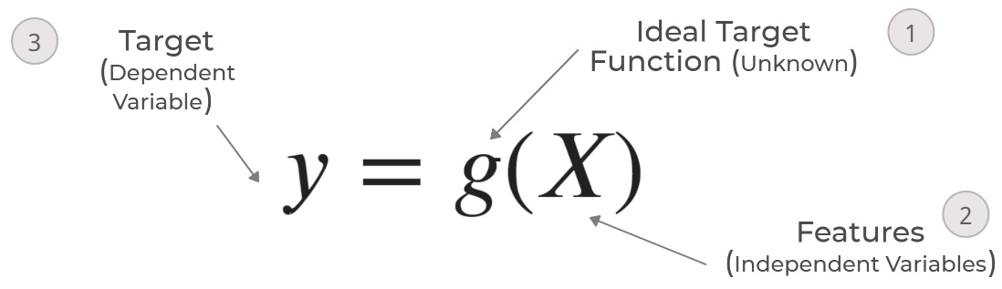
Figure 5.2 – Supervised machine learning schematic, part 1 – the ideal function

As we already discussed, what we want from machine learning is to learn from the data and come up with a set of rules/logic. The closest analogy in mathematics for logic/rules is a function, which takes in an input (here, data) and provides an output. Mathematically, it can be written as follows:

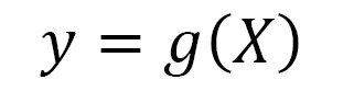
where X is the set of features and g is the ideal target function (denoted by 1 in Figure 5.2) that maps the X input (denoted by 2 in the schematic) to the target (ideal) output, y (denoted by 3 in the schematic). The ideal target function is largely an unknown function, similar to the data generating process (DGP) we saw in Chapter 1, Introducing Time Series, which is not in our control.

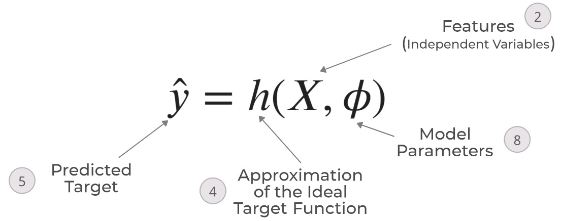
Figure 5.3 – Supervised machine learning schematic, part 2 – the learned approximation

But, we want the computer to learn this ideal target function. This approximation of the ideal target function is denoted by another function, h (4 in the schematic), which takes in the same set of features, X, and outputs a predicted target, (5 in the schematic). are the parameters of the h function (or model parameters):

Figure 5.4 – Supervised machine learning schematic, part 3 – putting it all together

Now, how do we find this approximation h function and its parameters, ? With the dataset of examples (6 in the schematic). The supervised machine learning problem works on the premise that we are able to collect a set of examples that shows the features, X, and the corresponding target, y, which is also referred to as labels in literature. It is from this set of examples (the dataset) that the computer learns the approximation function, h, and the optimal model parameters, . In the preceding diagram, the only real unknown entity is the ideal target function, g. So, we can use the training dataset, D, to get predicted targets for every sample in the dataset. We already know the ideal target for all the examples. We need a way to compare the ideal targets and predicted targets, and this is where the loss function (7 in the schematic) comes in. This loss function tells us how far away from the real truth we are with the approximated function, h.

Although h can be any function, it is typically chosen from a set of a well-known class of functions, . is the finite set of functions that can be fit to the data. This class of functions is what we colloquially call models. For instance, h can be chosen from all the linear functions or all the tree-based functions, and so on. Choosing an h from is done by a combination of hyperparameters (which the modeler specifies) and the model parameter, which is learned from data.

Now, all that is left is to run through the different functions so that we find the best approximation function, h, which gives us the lowest loss. This is an optimization process that we call training.

Let’s also take a look at a few key concepts, which will be important in all our discussions ahead.

Supervised machine learning tasks

Machine learning can be used to solve a wide variety of tasks such as regression, classification, and recommendation. But, since classification and regression are the most popular classes of problems, we will spend just a little bit of time reviewing what they are.

The difference between classification and regression tasks is very simple. In the machine learning schematic (Figure 5.2), we talked about y, the target. This target can be either a real-valued number or a class of items. For instance, we could be predicting the stock price for next week or we could just predict whether the stock was going to go up or down. In the first case, we are predicting a real-valued number, which is called regression. In the other case, we are predicting one out of two classes (up or down), and this is called classification.

Overfitting and underfitting

The biggest challenge in machine learning systems is that the model we trained must perform well on a new and unseen dataset. The ability of a machine learning model to do that is called the generalization capability of the model. The training process in a machine learning setup is akin to mathematical optimization, with one subtle difference. The aim of mathematical optimization is to arrive at the global maxima in the provided dataset. But in machine learning, the aim is to achieve low test error by using the training error as a proxy. How well a machine learning model is doing on training error and testing error is closely related to the concepts of overfitting and underfitting. Let’s use an example to understand these terms.

The learning process of a machine learning model has many parallels to how humans learn. Suppose three students, A, B, and C, are studying for an examination. A is a slacker and went clubbing the night before. B decided to double down and memorize the textbook end to end. And, C paid attention in class and understood the topics up for the examination.

As expected, A flunked the examination, C got the highest score, and B did OK.

A flunked the examination because they didn’t learn enough. This happens to machine learning models as well when they don’t learn enough patterns, and this is called underfitting. This is characterized by high training errors and high test errors.

B didn’t score as highly as expected; after all, they did memorize the whole text, word for word. But many questions in the examination weren’t directly from the textbook and B wasn’t able to answer them correctly. In other words, the questions in the examination were new and unseen. And because B memorized everything but didn’t make an effort to understand the underlying concepts, B wasn’t able to generalize the knowledge they had to new questions. This situation, in machine learning, is called overfitting. This is typically characterized by a big delta in training and test errors. Typically, we will see very low training errors and high test errors.

The third student, C, learned the right way and understood the underlying concepts and because of that, was able to generalize to new and unseen questions. This is the ideal state for a machine learning model, as well. This is characterized by reasonably low test errors and a small delta between training and test errors.

We just saw the two greatest challenges in machine learning. Now, let’s also look at a few ways we have that can be used to tackle these challenges.

There is a close relationship between the capacity of a model and underfitting or overfitting. A model’s capacity is its ability to be flexible enough to fit a wide variety of functions. Models with low capacity may struggle to fit the training data, leading to underfitting. Models with high capacity may overfit by memorizing the training data too much. Just to develop an intuition around this concept of capacity, let’s look at an example. When we move from linear regression to polynomial regression, we are adding more capacity to the model. Instead of fitting just straight lines, we are letting the model fit curved lines as well. Machine learning models generally do well when their capacity is appropriate for the learning problem at hand.

Figure 5.5 – Underfitting versus overfitting

Figure 5.5 shows a very popular case to illustrate overfitting and underfitting. We create a few random points using a known function and try to learn that by using those data samples. We can see that the linear regression, which is one of the simplest models, has underfitted the data by drawing a straight line through those points. Polynomial regression is linear regression, but with some higher-order features. For now, you can consider the move from linear regression to polynomial regression with higher degrees as increasing the capacity of the model. So, when we use a degree of 4, we see that the learned function fits the data well and matches our ideal function. But if we keep increasing the capacity of the model and reach degree = 15, we see that the learned function is still passing through the training samples, but has learned a very different function, overfitting to the training data. Finding the optimal capacity to learn a generalizable function is one of the core challenges of machine learning.

While capacity is one aspect of the model, another aspect is regularization. Even with the same capacity, there are multiple functions a model can choose from the hypothesis space of all functions. With regularization, we try to give preference to a set of functions in the hypothesis space over the others. While all these functions are valid functions that can be chosen, we nudge the optimization process in such a way that we end up with a kind of function toward which we have a preference. Although regularization is a general term used to refer to any kind of constraint we place on the learning process to reduce the complexity of the learned function, more commonly, it is used in the form of a weight decay. Let’s take an example of linear regression, which is when we fit a straight line to the input features by learning a weight associated with each feature.

A linear regression model can be written mathematically as follows:

Here, N is the number of features, c is the intercept, is the ith feature, and is the weight associated with the ith feature. We estimate the right weight (L) by considering this as an optimization problem that minimizes the error between and y (real output).

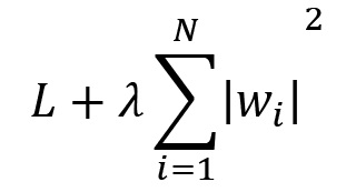
Now, with regularization, we add an additional term to L, which forces the weights to become smaller. Commonly, this is done using an l1 or l2 regularizer. An l1 regularizer is when you add the sum of squared weights to L:

where is the regularization coefficient that determines how strongly we penalize the weights. An l2 regularizer is when you add the sum of absolute weights to L:

In both cases, we are enforcing a preference for smaller weights over larger weights because it keeps the function from relying too much on any one feature from the ones used in the machine learning model. Regularization is an entire topic unto itself and if you want to learn more, head over to the Further reading section for a few resources on regularization.

Another really effective way to reduce overfitting is to simply train the model with more data. With a larger dataset, the chances of the model overfitting become less because of the sheer variety that can be captured in a large dataset.

Now, how do we tune the knobs to strike a balance between underfitting and overfitting? Let’s look at it in the following section.

Hyperparameters and validation sets

Almost all machine learning models have a few hyperparameters associated with them. Hyperparameters are parameters of the model that are not learned from data but rather are set before the start of training. For instance, the weight of the regularization is a hyperparameter. Most hyperparameters either help us control the capacity of the model or apply regularization to the model. By controlling either capacity or regularization or both, we can travel the frontier between underfitting and overfitting models and arrive at a model that is just right.

But since these hyperparameters have to be set outside of the algorithm, how do we estimate the best hyperparameters? Although it is not part of the core learning process, we learn the hyperparameters also from the data. But if we just use the training data to learn the hyperparameters, it will just choose the maximum possible model capacity, which results in overfitting. This is where we need a validation set, a part of the data that the training process does not have access to. But when the dataset is small (not hundreds of thousands of samples), the performance on a single validation set doesn’t guarantee a fair evaluation. In such cases, we rely on cross-validation. The general trick is to repeat the training and evaluation procedure on different subsets of the original dataset. A common way of doing this is called k-fold cross validation, when the original dataset is divided into k equal, non-overlapping, and random subsets, and each subset is evaluated after training on all the other subsets. We have provided a link in the Further reading section if you want to read up about cross-validation techniques. Later in the book, we will also be covering this topic, but from the time series perspective, which has a few differences from the standard way of doing cross-validation.

Suggested reading

Although we have touched the surface of machine learning in the book, there is a lot more, and to truly appreciate the rest of the book better, we suggest gaining more understanding of machine learning. We suggest starting with Machine Learning by Stanford (Andrew Ng) – https://www.coursera.org/learn/machine-learning. If you are in a hurry, the Machine Learning Crash Course by Google is also a good starting point – https://developers.google.com/machine-learning/crash-course/ml-intro.

Now that we have a basic understanding of machine learning, let’s start looking at how we can use it to do time series forecasting.

Time series forecasting as regression

A time series, as we saw in Chapter 1, Introducing Time Series, is a set of observations taken sequentially in time. And typically, time series forecasting is about trying to predict what these observations will be in the future. Given a sequence of observations of arbitrary length of history, we predict the future to an arbitrary horizon.

We saw that regression, or machine learning to predict a continuous variable, works on a dataset of examples, and each example is a set of input features and targets. We can see that regression, which is tasked with predicting a single output provided with a set of inputs, is fundamentally incompatible with forecasting, where we are given a set of historical values and asked to predict the future values. This fundamental incompatibility between the time series and machine learning regression paradigms is why we cannot use regression for time series forecasting directly.

Moreover, time series forecasting, by definition, is an extrapolation problem, whereas regression, most of the time, is an interpolation one. Extrapolation is typically harder to solve using data-driven methods. Another key assumption in regression problems is that the samples used for training are independent and identically distributed (IID). But time series break that assumption as well because subsequent observations in a time series display considerable dependence.

However, to use the wide variety of techniques from machine learning, we need to cast time series forecasting as a regression. Thankfully, there are ways to convert a time series into a regression and get over the IID assumption by introducing some memory to the machine learning model through some features. Let’s see how it can be done.

Time delay embedding

We talked about the ARIMA model in Chapter 4, Setting a Strong Baseline Forecast, and saw how it is an autoregressive model. We can use the same concept to convert a time series problem into a regression one. Let’s use the following diagram to make the concept clear:

Figure 5.6 – Time series to regression conversion using a sliding window

Let’s assume we have a time series with time steps, . Consider we are at time t, and we have a time series of the length of history as L. So, our time series will look something like in the diagram with as the latest observation in the time series, and and so on as we move backward in time.

In an ideal world, each observation in should be conditioned on all the previous observations when we forecast. But, it is not practical because L can be arbitrarily long. We often restrict the forecasting function to use only the most recent M observations of the series, where M < L. These are called finite memory models or Markov models and M is called the order of autoregression, memory size, or the receptive field.

Therefore, in time delay embedding, we assume a window of arbitrary length M < L and extract fixed-length subsequences from the time series by sliding the window over the length of the time series.

In the diagram, we have taken a sliding window with a memory size of 3. So, the first subsequence we can extract (if we are starting from the most recent and working backward) is . And is the observation that comes right after the subsequence. This becomes our first example in the dataset (row 1 in the table in the diagram). Now, we slide the window one time step to the left (backward in time) and extract the new subsequence, . The corresponding target would become . We repeat this process as we move back to the beginning of the time series, and at each step of the sliding window, we add one more example to the dataset.

At the end of it, we have an aligned dataset with a fixed vector size of features (which will be equal to the window size) and a single target, which is what a typical machine learning dataset looks like.

Now that we have a table with three features, let’s also assign semantic meaning to the three features. If we look at the right-most column in the table in the diagram, we can see that the time step present in the column is always one time step behind the target. We call it Lag 1. The second column from the right is always two time steps behind the target, and this is called Lag 2. Generalizing this, the feature that has observations that are n time steps behind the target, we call Lag n.

This transformation from time series to regression using time-delay embedding encodes the autoregressive structure of a time series in a way that can be utilized by standard regression frameworks. Another way we can think about using regression for time series forecasting is to perform regression on time.

Temporal embedding

If we rely on previous observations in autoregressive models, we rely on the concept of time for temporal embedding models. The core idea is that we forget the autoregressive nature of the time series and assume that any value in the time series is only dependent on time. We derive features that capture time, the passage of time, periodicity of time, and so on, from the timestamps associated with the time series, and then we use these features to predict the target using a regression model. There are many ways to do this, from simply aligning a monotonically and uniformly increasing numerical column that captures the passage of time to sophisticated Fourier terms to capture the periodic components in time. We will talk about those techniques in detail in Chapter 6, Feature Engineering for Time Series Forecasting.

Before we wind up the chapter, let’s also talk about a key concept that is gaining ground steadily in the time series forecasting space. A large part of this book embraces this new paradigm of forecasting.

Global forecasting models – a paradigm shift

Traditionally, each time series was treated in isolation. Because of that, traditional forecasting has always looked at the history of a single time series alone in fitting a forecasting function. But recently, because of the ease of collecting data in today’s digital-first world, many companies have started collecting large amounts of time series from similar sources, or related time series.

For example, retailers such as Walmart collect data on sales of millions of products across thousands of stores. Companies such as Uber or Lyft collect the demand for rides from all the zones in a city. In the energy sector, energy consumption data is collected across all consumers. All these sets of time series have shared behavior and are hence called related time series.

We can consider that all the time series in a related time series come from separate data generating processes (DGPs), and thereby model them all separately. We call these the local models of forecasting. An alternative to this approach is to assume that all the time series are coming from a single DGP. Instead of fitting a separate forecast function for each time series individually, we fit a single forecast function to all the related time series. This approach has been called global or cross-learning in literature.

Reference check

The terminology global was introduced by David Salinas et al. in the DeepAR paper (reference number 1) and Cross-learning by Slawek Smyl (reference number 2).

We saw earlier that having more data will lead to lower chances of overfitting and, therefore, lower generalization error (the difference between training and testing errors). This is exactly one of the shortcomings of the local approach. Traditionally, time series are not very long, and in many cases, it is difficult and time-consuming to collect more data as well. Fitting a machine learning model (with all its expressiveness) on small data is prone to overfitting. This is why time series models that enforce strong priors were used to forecast such time series, traditionally. But these strong priors, which restrict the fitting of traditional time series models, can also lead to a form of underfitting and limit accuracy.

Strong and expressive data-driven models, as in machine learning, require a larger amount of data to have a model that generalizes to new and unseen data. A time series, by definition, is tied to time, and sometimes, collecting more data means waiting for months or years and that is not desirable. So, if we cannot increase the length of the time-series dataset, we can increase the width of the time series dataset. If we add multiple time series to the dataset, we increase the width of the dataset, and there by increase the amount of data the model is getting trained with. Figure 5.7 shows the concept of increasing the width of a time series dataset visually:

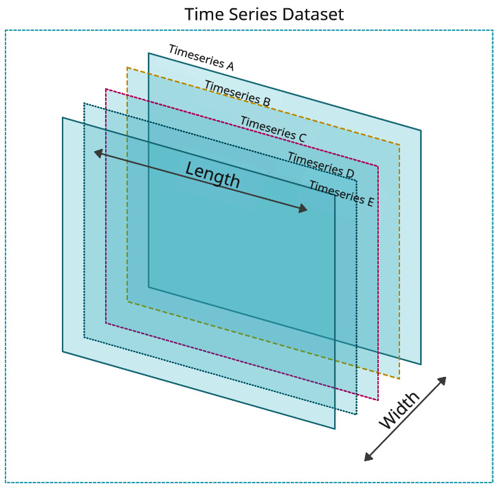
Figure 5.7 – The length and width of a time series dataset

This works in favor of machine learning models because with higher flexibility in fitting a forecast function and the addition of more data to work with, the machine learning model can learn a more complex forecast function than traditional time series models, which are typically shared between the related time series, in a completely data-driven way.

Another shortcoming of the local approach revolves around scalability. In the case of Walmart we mentioned earlier, there are millions of time series that need to be forecasted and it is not possible to have human oversight on all these models. If we think about this from an engineering perspective, training and maintaining millions of models in a production system would give any engineer a nightmare. But under the global approach, we only train a single model for all these time series, which drastically reduces the number of models we need to maintain and yet can generate all the required forecasts.

This new paradigm of forecasting has gained traction and has consistently been shown to improve the local approaches in multiple time series competitions, mostly in datasets of related time series. In Kaggle competitions, such as Rossman Store Sales (2015), Wikipedia WebTraffic Time Series Forecasting (2017), Corporación Favorita Grocery Sales Forecasting (2018), and M5 Competition (2020), the winning entries were all global models—either machine learning or deep learning or a combination of both. The Intermarché Forecasting Competition (2021) also had global models as the winning submissions. Links to these competitions are provided in the Further reading section.

Although we have many empirical findings where the global models have outperformed local models for related time series, global models are still a relatively new area of research. Montero-Manson and Hyndman (2020) showed a few very interesting results and showed that any local method can be approximated by a global model with required complexity, and the most interesting finding they put forward is that the global model will perform better, even with unrelated time series. We will talk more about global models and strategies for global models in Chapter 10, Global Forecasting Models.

Reference check

The Montero-Manson and Hyndman (2020) research paper is cited in References under reference number 3.

Summary

We have started our journey beyond baseline forecasting methods and dipped our toes into the world of machine learning. After a brief refresher on machine learning, where we looked at key concepts such as overfitting, underfitting, regularization, and so on, we saw how we can convert a time series forecasting problem into a regression problem from the machine learning world. We also developed a conceptual understanding of different embeddings, such as time delay embedding and temporal embedding, which can be used to convert a time series problem into a regression problem. To wrap things up, we also learned about a new paradigm in time series forecasting – global models – and contrasted them with local models on a conceptual level. In the next few chapters, we will start putting these concepts into practice, and see techniques for feature engineering, and strategies for global models.

References

Following are the references that we used in this chapter:

1. David Salinas, Valentin Flunkert, Jan Gasthaus, Tim Januschowski (2020). DeepAR: Probabilistic forecasting with autoregressive recurrent networks. International Journal of Forecasting. 36-3. 1181-1191: https://doi.org/10.1016/j.ijforecast.2019.07.001
2. Slawek Smyl (2020). A hybrid method of exponential smoothing and recurrent neural networks for time series forecasting. International Journal of Forecasting. 36-1: 75-85 https://doi.org/10.1016/j.ijforecast.2019.03.017
3. Montero-Manso, P., Hyndman, R.J.. (2020), Principles and algorithms for forecasting groups of time series: Locality and globality. arXiv:2008.00444[cs.LG]: https://arxiv.org/abs/2008.00444

Further reading

You can check out the following resources for further reading:

• Regularization for Sparsity from Google Machine Learning Crash Course: https://developers.google.com/machine-learning/crash-course/regularization-for-sparsity/l1-regularization
• L1 and L2 Regularization from Foundations of Machine Learning, Bloomberg ML EDU: https://www.youtube.com/watch?v=d6XDOS4btck
• Cross-validation: evaluating estimator performance from scikit-learn: https://scikit-learn.org/stable/modules/cross_validation.html
• Rossmann Store Sales: https://www.kaggle.com/c/rossmann-store-sales
• Web Traffic Time Series Forecasting – https://www.kaggle.com/c/web-traffic-time-series-forecasting
• Corporación Favorita Grocery Sales Forecasting – https://www.kaggle.com/c/favorita-grocery-sales-forecasting
• M5 Forecasting – Accuracy – https://www.kaggle.com/c/m5-forecasting-accuracy