
1
Introducing Time Series
Welcome to Advanced Time Series Analysis Using Python! This book is intended for data scientists or machine learning (ML) engineers who want to level up their time series analysis skills by learning new and advanced techniques from the ML world. Time series analysis is something that is commonly overlooked in regular ML books, courses, and so on. They typically start with classification, touch upon regression, and then move on. But it is also something that is immensely valuable and ubiquitous in business. As long as time is one of the four dimensions in the world we live in, time series data is all-pervasive.
Analyzing time series data unlocks a lot of value for a business. Time series analysis isn't new—it's been around since the 1920s and 1930s. But in the current age of data, the time series that are collected by businesses are growing larger and wider by the minute. Combined with an explosion in the quantum of data collected and the renewed interest in ML, the landscape of time series analysis also changed considerably. This book attempts to take you beyond classical statistical methods such as AutoRegressive Integrated Moving Average (ARIMA) and introduce to you the latest techniques from the ML world in time series analysis.
We are going to start with the basics and quickly scale up to more complex topics. In this chapter, we're going to cover the following main topics:
- What is a time series?
- Data-generating process (DGP)
- What can we forecast?
- Forecasting terminology and notation
Technical requirements
You will need to set up the Anaconda environment following the instructions in the Preface of the book to get a working environment with all the packages and datasets required for the code in this book.
The associated code for the chapter can be found at https://github.com/PacktPublishing/Modern-Time-Series-Forecasting-with-Python-/tree/main/notebooks/Chapter01.
What is a time series?
To keep it simple, a time series is a set of observations taken sequentially in time. The focus is on the word time. If we keep taking the same observation at different points in time, we will get a time series. For example, if you keep recording the number of bars of chocolate you have in a month, you'll end up with a time series of your chocolate consumption. Suppose you are recording your weight at the beginning of every month. You get another time series of your weight. Is there any relation between the two time series? Most likely, yeah. But we can analyze that scientifically by the end of this book.
A few other examples of time series are the weekly closing price of a stock that you follow, daily rainfall or snow in your city, or hourly readings of your heartbeat from your smartwatch.
Types of time series
There are two types of time series data, as outlined here:
- Regular time series: This is the most common type of time series where we have observations coming in at regular intervals of time, such as every hour or every month.
- Irregular time series: There are a few time series where we do not have observations at a regular interval of time. For example, consider we have a sequence of readings from lab tests of a patient. We see an observation in the time series only when the patient heads to the clinic and carries out the lab test, and this may not happen in regular intervals of time.
Important note
This book only focuses on regular time series, which are evenly spaced in time. Irregular time series are slightly more advanced and require specialized techniques to handle them. A couple of survey papers on the topic is a good way to get started on irregular time series and you can find them in the Further reading section of this chapter.
Main areas of application for time series analysis
There are broadly three important areas of application for time series analysis, outlined as follows:
- Time series forecasting: Predicting the future values of a time series, given the past values—for example, predict the next day's temperature using the last 5 years of temperature data.
- Time series classification: Sometimes, instead of predicting the future value of the time series, we may also want to predict an action based on past values. For example, given a history of an electroencephalogram (EEG; tracking electrical activity in the brain) or an electrocardiogram (EKG; tracking electrical activity in the heart), we need to predict whether the result of an EEG or an EKG is normal or abnormal.
- Interpretation and causality: Understand the whats and whys of the time series based on the past values, understand the interrelationships among several related time series, or derive causal inference based on time series data.
Important note
The focus of this book is predominantly on time series forecasting, but the techniques that you learn will help you approach time series classification problems also, with minimal change in the approach. Interpretation is also addressed, although only briefly, but causality is an area that this book does not address because it warrants a whole different approach.
Now that we have an overview of the time series landscape, let's build a mental model on how time series data is generated.
Data-generating process (DGP)
We saw that time series data is a collection of observations made sequentially along the time dimension. Any time series is, in turn, generated by some kind of mechanism. For example, time series data of daily shipments of your favorite chocolate from the manufacturing plant is affected by a lot of factors such as the time of the year, the holiday season, the availability of cocoa, the uptime of the machines working on the plant, and so on. In statistics, this underlying process that generated the time series is referred to as the DGP. Often, time series data is generated by a stochastic process.
If we had complete and perfect knowledge of reality, all we must do is put this DGP together in a mathematical form and you will get the most accurate forecast possible. But sadly, nobody has complete and perfect knowledge of reality. So, what we try to do is approximate the DGP, mathematically, as much as possible so that our imitation of the DGP gives us the best possible forecast (or any other output we want from the analysis). This imitation is called a model that provides a useful approximation to the DGP.
But we must remember that the model is not the DGP, but a representation of some essential aspects of reality. For example, let's consider an aerial view of Bengaluru and a map of Bengaluru, as represented here:

Figure 1.1 – An aerial view of Bengaluru (left) and a map of Bengaluru (right)
The map of Bengaluru is certainly useful—we can use it to go from point A to point B. But a map of Bengaluru is not the same as a photo of Bengaluru. It doesn't showcase the bustling nightlife or the insufferable traffic. A map is just a model that represents some useful features of a location, such as roads and places. The following diagram might help us internalize the concept and remember it:
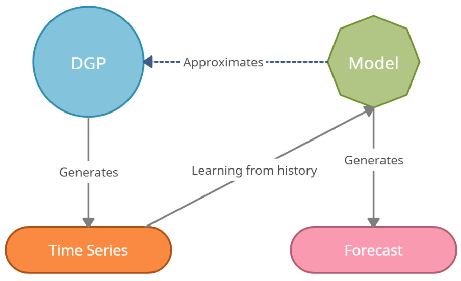
Figure 1.2 – DGP, model, and time series
Naturally, the next question would be this: Do we have a useful model? Every model is unrealistic. As we saw already, a map of Bengaluru does not perfectly represent Bengaluru. But if our purpose is to navigate Bengaluru, then a map is a very useful model. What if we want to understand the culture? A map doesn't give you a flavor of that. So, now, the same model that was useful is utterly useless in the new context.
Different kinds of models are required in different situations and for different objectives. For example, the best model for forecasting may not be the same as the best model to make a causal inference.
We can use the concept of DGPs to generate multiple synthetic time series, of varying degrees of complexity.
Generating synthetic time series
Let's take a look at a few practical examples where we can generate a few time series using a set of fundamental building blocks. You can get creative and mix and match any of these components, or even add them together to generate a time series of arbitrary complexity.
White and red noise
An extreme case of a stochastic process that generates a time series is a white noise process. It has a sequence of random numbers with zero mean and constant standard deviation. This is also one of the most popular assumptions of noise in a time series.
Let's see how we can generate such a time series and plot it, as follows:
# Generate the time axis with sequential numbers upto 200
time = np.arange(200)
# Sample 200 hundred random values
values = np.random.randn(200)*100
plot_time_series(time, values, "White Noise")
Here is the output:
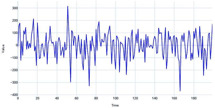
Figure 1.3 – White noise process
Red noise, on the other hand, has zero mean and constant variance but is serially correlated in time. This serial correlation or redness is parameterized by a correlation coefficient r, such that:

where w is a random sample from a white noise distribution.
Let's see how we can generate that, as follows:
# Setting the correlation coefficient
r = 0.4
# Generate the time axis
time = np.arange(200)
# Generate white noise
white_noise = np.random.randn(200)*100
# Create Red Noise by introducing correlation between subsequent values in the white noise
values = np.zeros(200)
for i, v in enumerate(white_noise):
    if i==0:
        values[i] = v
    else:
        values[i] = r*values[i-1]+ np.sqrt((1-np.power(r,2))) *v
plot_time_series(time, values, "Red Noise Process")
Here is the output:
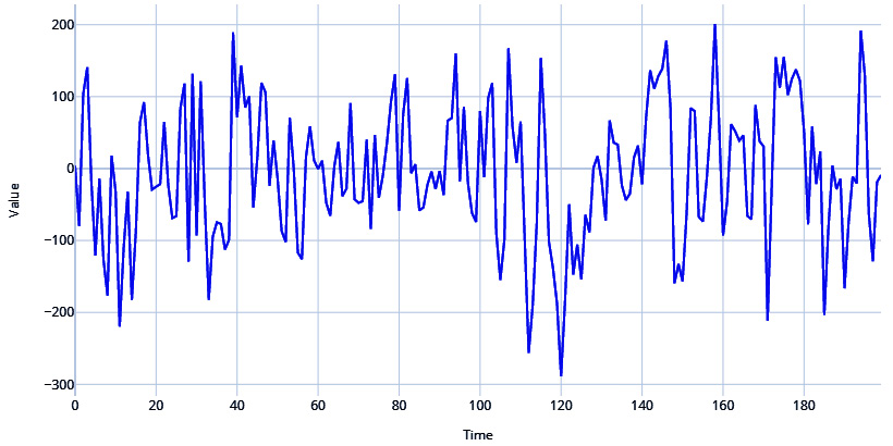
Figure 1.4 – Red noise process
Cyclical or seasonal signals
Among the most common signals you see in time series are seasonal or cyclical signals. Therefore, you can introduce seasonality into your generated series in a few ways.
Let's take the help of a very useful library to generate the rest of the time series—TimeSynth. For more information, refer to https://github.com/TimeSynth/TimeSynth.
This is a very useful library to generate time series. It has all kinds of DGPs that you can mix and match and create authentic synthetic time series.
Important note
For the exact code and usage, please refer to the associated Jupyter notebooks.
Let's see how we can use a sinusoidal function to create cyclicity. There is a helpful function in TimeSynth called generate_timeseries that helps us combine signals and generate time series. Have a look at the following code snippet:
#Sinusoidal Signal with Amplitude=1.5 & Frequency=0.25
signal_1 =ts.signals.Sinusoidal(amplitude=1.5, frequency=0.25)
#Sinusoidal Signal with Amplitude=1 & Frequency=0. 5
signal_2 = ts.signals.Sinusoidal(amplitude=1, frequency=0.5)
#Generating the time series
samples_1, regular_time_samples, signals_1, errors_1 = generate_timeseries(signal=signal_1)
samples_2, regular_time_samples, signals_2, errors_2 = generate_timeseries(signal=signal_2)
plot_time_series(regular_time_samples,
                 [samples_1, samples_2],
                 "Sinusoidal Waves",
                 legends=["Amplitude = 1.5 | Frequency = 0.25", "Amplitude = 1 | Frequency = 0.5"])
Here is the output:
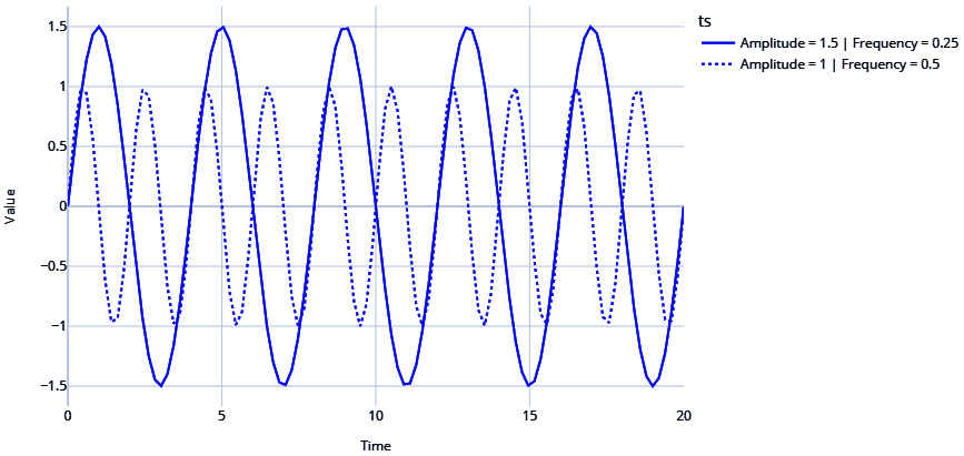
Figure 1.5 – Sinusoidal waves
Note the two sinusoidal waves are different with respect to the frequency (how fast the time series crosses zero) and amplitude (how far away from zero the time series travels).
TimeSynth also has another signal called PseudoPeriodic. This is like the Sinusoidal class, but the frequency and amplitude itself has some stochasticity. We can see in the following code snippet that this is more realistic than the vanilla sine and cosine waves from the Sinusoidal class:
# PseudoPeriodic signal with Amplitude=1 & Frequency=0.25
signal = ts.signals.PseudoPeriodic(amplitude=1, frequency=0.25)
#Generating Timeseries
samples, regular_time_samples, signals, errors = generate_timeseries(signal=signal)
plot_time_series(regular_time_samples,
                 samples,
                 "Pseudo Periodic")
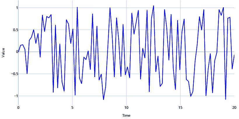
Figure 1.6 – Pseudo-periodic signal
Autoregressive signals
Another very popular signal in the real world is an autoregressive (AR) signal. We will go into this in more detail in Chapter 4, Setting a Strong Baseline Forecast, but for now, an AR signal refers to when the value of a time series for the current timestep is dependent on the values of the time series in the previous timesteps. This serial correlation is a key property of the AR signal, and it is parametrized by a few parameters, outlined as follows:
- Order of serial correlation—or, in other words, the number of previous timesteps the signal is dependent on
- Coefficients to combine the previous timesteps
Let's see how we can generate an AR signal and see what it looks like, as follows:
# Autoregressive signal with parameters 1.5 and -0.75
# y(t) = 1.5*y(t-1) - 0.75*y(t-2)
signal=ts.signals.AutoRegressive(ar_param=[1.5, -0.75])
#Generate Timeseries
samples, regular_time_samples, signals, errors = generate_timeseries(signal=signal)
plot_time_series(regular_time_samples,
                 samples,
                 "Auto Regressive")
Here is the output:
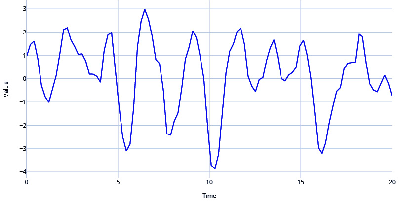
Figure 1.7 – AR signal
Mix and match
There are many more components you can use to create your DGP and thereby generate a time series, but let's quickly look at how we can combine the components we have already seen to generate a realistic time series.
Let's use a pseudo-periodic signal with white noise and combine it with an AR signal, as follows:
#Generating Pseudo Periodic Signal
pseudo_samples, regular_time_samples, _, _ = generate_timeseries(signal=ts.signals.PseudoPeriodic(amplitude=1, frequency=0.25), noise=ts.noise.GaussianNoise(std=0.3))
# Generating an Autoregressive Signal
ar_samples, regular_time_samples, _, _ = generate_timeseries(signal=ts.signals.AutoRegressive(ar_param=[1.5, -0.75]))
# Combining the two signals using a mathematical equation
ts = pseudo_samples*2+ar_samples
plot_time_series(regular_time_samples,
                 ts,
                 "Pseudo Periodic with AutoRegression and White Noise")
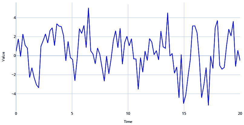
Figure 1.8 – Pseudo-periodic signal with AR and white noise
Stationary and non-stationary time series
In time series, stationarity is of great significance and is a key assumption in many modeling approaches. Ironically, many (if not most) real-world time series are non-stationary. So, let's understand what a stationary time series is from a layman's point of view.
There are multiple ways to look at stationarity, but one of the clearest and most intuitive ways is to think of the probability distribution or the data distribution of a time series. We call a time series stationary when the probability distribution remains the same at every point in time. In other words, if you pick different windows in time, the data distribution across all those windows should be the same.
A standard Gaussian distribution is defined by two parameters—the mean and the standard deviation. So, there are two ways the stationarity assumption can be broken, as outlined here:
- Change in mean over time
- Change in variance over time
Let's look at these assumptions in detail and understand them better.
Change in mean over time
This is the most popular way a non-stationary time series presents itself. If there is an upward/downward trend in the time series, the mean across two windows of time would not be the same.
Another way non-stationarity manifests itself is in the form of seasonality. Suppose we are looking at the time series of average temperature measurements in a month for the last 5 years. From our experience, we know that temperature peaks during summer and falls in winter. So, when we take the mean temperature of winter and mean temperature of summer, they will be different.
Let's generate a time series with trend and seasonality and see how it manifests, as follows:
# Sinusoidal Signal with Amplitude=1 & Frequency=0.25
signal=ts.signals.Sinusoidal(amplitude=1, frequency=0.25)
# White Noise with standard deviation = 0.3
noise=ts.noise.GaussianNoise(std=0.3)
# Generate the time series
sinusoidal_samples, regular_time_samples, _, _ = generate_timeseries(signal=signal, noise=noise)
# Regular_time_samples is a linear increasing time axis and can be used as a trend
trend = regular_time_samples*0.4
# Combining the signal and trend
ts = sinusoidal_samples+trend
plot_time_series(regular_time_samples,
                 ts,
                 "Sinusoidal with Trend and White Noise")
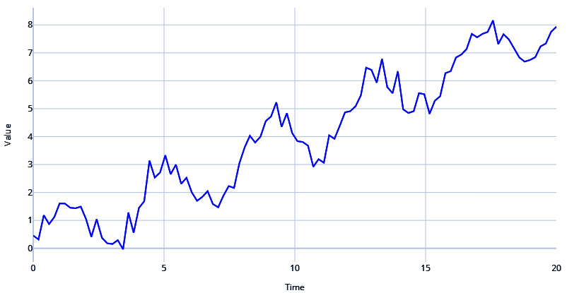
Figure 1.9 – Sinusoidal signal with trend and white noise
If you examine the time series in Figure 1.9, you will be able to see a definite trend and the seasonality, which together make the mean of the data distribution change wildly across different windows of time.
Change in variance over time
Non-stationarity can also present itself in the fluctuating variance of a time series. If the time series starts off with low variance and as time progresses, the variance keeps getting bigger and bigger, we have a non-stationary time series. In statistics, there is a scary name for this phenomenon—heteroscedasticity.
This book just tries to give you intuition about stationary versus non-stationary time series. There is a lot of statistical theory and depth in this discussion that we are skipping over to keep our focus on the practical aspects of time series.
Armed with the mental model of the DGP, we are at the right place to think about another important question: What can we forecast?
What can we forecast?
Before we move ahead, there is another aspect of time series forecasting that we have to understand—the predictability of a time series. The most basic assumption when we forecast a time series is that the future depends on the past. But not all time series are equally predictable.
Let's take a look at a few examples and try to rank these in order of predictability (from easiest to hardest), as follows:
- High tide next Monday
- Lottery numbers next Sunday
- The stock price of Tesla next Friday
Intuitively, it is very easy for us to rank them. High tide next Monday is going to be the easiest to predict because it is so predictable, the lottery numbers are going to be very hard to predict because these are pretty much random, and the stock price of Tesla next Friday is going to be difficult to predict, but not impossible.
Note
However, for people thinking that they can forecast stock prices with the awesome techniques covered in the book and get rich, that won't happen. Although it is worthy of a lengthy discussion, we can summarize the key points in a short paragraph.
Share prices are not a function of their past values but an anticipation of their future values, and this thereby violates our first assumption while forecasting. And if that is not bad enough, financial stock prices typically have a very low signal-to-noise ratio. The final wrench in the process is the efficient-market hypothesis (EMH). This seemingly innocent hypothesis proclaims that all known information about a stock price is already factored into the price of the stock. The implication of the hypothesis is that if you can forecast accurately, many others will also be able to do that, and thereby the market price of the stock already reflects the change in price that this forecast brought about.
Coming back to the topic at hand—predictability—three main factors form a mental model for this, as follows:
- Understanding the DGP: The better you understand the DGP, the higher the predictability of a time series.
- Amount of data: The more data you have, the better your predictability is.
- Adequately repeating pattern: For any mathematical model to work well, there should be an adequately repeating pattern in your time series. The more repeatable the pattern is, the better your predictability is.
Even though you have a mental model of how to think about predictability, we will look at more concrete ways of assessing the predictability of time series in Chapter 3, Analyzing and Visualizing Time Series Data, but the key takeaway is that not all time series are equally predictable.
In order to fully follow the discussion in the coming chapters, we need to establish a standard notation and get updated on terminology that is specific to time series analysis.
Forecasting terminology
There are a few terminologies that will help you follow the book as well as other literature on time series. These are described in more detail here:
- Forecasting
Forecasting is the prediction of future values of a time series using the known past values of the time series and/or some other related variables. This is very similar to prediction in ML where we use a model to predict unseen data.
- Multivariate forecasting
Multivariate time series consist of more than one time series variable that is not only dependent on its past values but also has some dependency on the other variables. For example, a set of macroeconomic indicators such as gross domestic product (GDP), inflation, and so on of a particular country can be considered as a multivariate time series. The aim of multivariate forecasting is to come up with a model that captures the interrelationship between the different variables along with its relationship with its past and forecast all the time series together in the future.
- Explanatory forecasting
In addition to the past values of a time series, we might use some other information to predict the future values of a time series. For example, for predicting retail store sales, information regarding promotional offers (both historical and future ones) is usually helpful. This type of forecasting, which uses information other than its own history, is called explanatory forecasting.
- Backtesting
Setting aside a validation set from your training data to evaluate your models is a practice that is common in the ML world. Backtesting is the time series equivalent of validation, whereby you use the history to evaluate a trained model. We will cover the different ways of doing validation and cross-validation for time series data later.
- In-sample and out-sample
Again, drawing parallels with ML, in-sample refers to training data and out-sample refers to unseen or testing data. When you hear in-sample metrics, this is referring to metrics calculated on training data, and out-sample metrics is referring to metrics calculated on testing data.
- Exogenous and endogenous variables
Exogenous variables are parallel time series variables that are not modeled directly for output but used to help us model the time series that we are interested in. Typically, exogenous variables are not affected by other variables in the system. Endogenous variables are variables that are affected by other variables in the system. A purely endogenous variable is a variable that is entirely dependent on the other variables in the system. Relaxing the strict assumptions a bit, we can consider the target variable as the endogenous variable and the explanatory regressors we include in the model as exogenous variables.
- Forecast combination
Forecast combinations in the time series world are similar to ensembling from the ML world. It is a process by which we combine multiple forecasts by using some function, either learned or heuristic-based, such as a simple average of three forecast models.
There are a lot more terms specific to time series, some of which we will be covering throughout the book. But to start with a basic familiarity in the field, these terms should be enough.
Summary
We had our first dip into time series as we understood the different types of time series, looked at how a DGP generates a time series, and saw how we can think about the important question: How well can we forecast a time series? We also had a quick review of the terminology and notation required to understand the rest of the book. In the next chapter, we will be getting our hands dirty and will learn how to work with time series data, how to preprocess a time series, how to handle missing data and outliers, and so on. If you have not set up the environment yet, take a break and put some time into doing that.
Further reading
- A Survey on Principles, Models and Methods for Learning from Irregularly Sampled Time Series: From Discretization to Attention and Invariance by S.N. Shukla and B.M. Marlin (2020): https://arxiv.org/abs/2012.00168
- Learning from Irregularly-Sampled Time Series: A Missing Data Perspective by S.C. Li and B.M. Marlin (2020), ICML: https://arxiv.org/abs/2008.07599
Introducing Time Series