Chapter 7. Parallel data processing and performance
- Processing data in parallel with parallel streams
- Performance analysis of parallel streams
- The fork/join framework
- Splitting a stream of data using a Spliterator
In the last three chapters, you’ve seen how the new Streams interface lets you manipulate collections of data in a declarative way. We also explained that the shift from external to internal iteration enables the native Java library to gain control over processing the elements of a stream. This approach relieves Java developers from explicitly implementing optimizations necessary to speed up the processing of collections of data. By far the most important benefit is the possibility of executing a pipeline of operations on these collections that automatically makes use of the multiple cores on your computer.
For instance, before Java 7, processing a collection of data in parallel was extremely cumbersome. First, you needed to explicitly split the data structure containing your data into subparts. Second, you needed to assign each of these subparts to a different thread. Third, you needed to synchronize them opportunely to avoid unwanted race conditions, wait for the completion of all threads, and finally combine the partial results. Java 7 introduced a framework called fork/join to perform these operations more consistently and in a less error-prone way. We’ll explore this framework in section 7.2.
In this chapter, you’ll discover how the Streams interface gives you the opportunity to execute operations in parallel on a collection of data without much effort. It lets you declaratively turn a sequential stream into a parallel one. Moreover, you’ll see how Java can make this magic happen or, more practically, how parallel streams work under the hood by employing the fork/join framework introduced in Java 7. You’ll also discover that it’s important to know how parallel streams work internally, because if you ignore this aspect, you could obtain unexpected (and likely wrong) results by misusing them.
In particular, we’ll demonstrate that the way a parallel stream gets divided into chunks, before processing the different chunks in parallel, can in some cases be the origin of these incorrect and apparently unexplainable results. For this reason, you’ll learn how to take control of this splitting process by implementing and using your own Spliterator.
7.1. Parallel streams
In chapter 4, we briefly mentioned that the Streams interface allows you to process its elements in parallel in a convenient way: it’s possible to turn a collection into a parallel stream by invoking the method parallelStream on the collection source. A parallel stream is a stream that splits its elements into multiple chunks, processing each chunk with a different thread. Thus, you can automatically partition the workload of a given operation on all the cores of your multicore processor and keep all of them equally busy. Let’s experiment with this idea by using a simple example.
Let’s suppose you need to write a method accepting a number n as argument and returning the sum of the numbers from one to n. A straightforward (perhaps naïve) approach is to generate an infinite stream of numbers, limiting it to the passed numbers, and then reduce the resulting stream with a BinaryOperator that sums two numbers, as follows:
public long sequentialSum(long n) {
    return Stream.iterate(1L, i -> i + 1)       1
                 .limit(n)                      2
                 .reduce(0L, Long::sum);        3
}
- 1 Generates the infinite stream of natural numbers
- 2 Limits it to the first n numbers
- 3 Reduces the stream by summing all the numbers
In more traditional Java terms, this code is equivalent to its iterative counterpart:
public long iterativeSum(long n) {
    long result = 0;
    for (long i = 1L; i <= n; i++) {
        result += i;
    }
    return result;
}
This operation seems to be a good candidate to use parallelization, especially for large values of n. But where do you start? Do you synchronize on the result variable? How many threads do you use? Who does the generation of numbers? Who adds them up?
Don’t worry about all of this. It’s a much simpler problem to solve if you adopt parallel streams!
7.1.1. Turning a sequential stream into a parallel one
You can make the former functional reduction process (summing) run in parallel by turning the stream into a parallel one; call the method parallel on the sequential stream:
public long parallelSum(long n) {
    return Stream.iterate(1L, i -> i + 1)
                 .limit(n)
                 .parallel()                     1
                 .reduce(0L, Long::sum);
}
- 1 Turns the stream into a parallel one
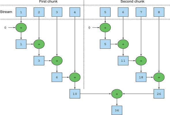
In the previous code, the reduction process used to sum all the numbers in the stream works in a way that’s similar to what’s described in section 5.4.1. The difference is that the stream is now internally divided into multiple chunks. As a result, the reduction operation can work on the various chunks independently and in parallel, as shown in figure 7.1. Finally, the same reduction operation combines the values resulting from the partial reductions of each substream, producing the result of the reduction process on the whole initial stream.
Figure 7.1. A parallel reduction operation
Note that, in reality, calling the method parallel on a sequential stream doesn’t imply any concrete transformation on the stream itself. Internally, a boolean flag is set to signal that you want to run in parallel all the operations that follow the invocation to parallel. Similarly, you can turn a parallel stream into a sequential one by invoking the method sequential on it. Note that you might think that by combining these two methods you could achieve finer-grained control over which operations you want to perform in parallel and which ones sequentially while traversing the stream. For example, you could do something like the following:
    stream.parallel()
          .filter(...)
          .sequential()
          .map(...)
          .parallel()
          .reduce();
But the last call to parallel or sequential wins and affects the pipeline globally. In this example, the pipeline will be executed in parallel because that’s the last call in the pipeline.
Looking at the stream’s parallel method, you may wonder where the threads used by the parallel stream come from, how many there are, and how you can customize the process.
Parallel streams internally use the default ForkJoinPool (you’ll learn more about the fork/join framework in section 7.2), which by default has as many threads as you have processors, as returned by Runtime.getRuntime().available-Processors().
But you can change the size of this pool using the system property java.util.concurrent.ForkJoinPool.common.parallelism, as in the following example:
System.setProperty("java.util.concurrent.ForkJoinPool.common.parallelism",
     "12");
This is a global setting, so it will affect all the parallel streams in your code. Conversely, it currently isn’t possible to specify this value for a single parallel stream. In general, having the size of the ForkJoinPool equal to the number of processors on your machine is a meaningful default, and we strongly suggest that you not modify it unless you have a good reason for doing so.
Returning to the number-summing exercise, we said that you can expect a significant performance improvement in its parallel version when running it on a multicore processor. You now have three methods executing exactly the same operation in three different ways (iterative style, sequential reduction, and parallel reduction), so let’s see which is the fastest one!
7.1.2. Measuring stream performance
We claimed that the parallelized summing method should perform better than the sequential and the iterative methods. Nevertheless, in software engineering, guessing is never a good idea! When optimizing performance, you should always follow three golden rules: measure, measure, measure. To this purpose we will implement a microbenchmark using a library called Java Microbenchmark Harness (JMH). This is a toolkit that helps to create, in a simple, annotation-based way, reliable microbenchmarks for Java programs and for any other language targeting the Java Virtual Machine (JVM). In fact, developing correct and meaningful benchmarks for programs running on the JVM is not an easy task, because there are many factors to consider like the warm-up time required by HotSpot to optimize the bytecode and the overhead introduced by the garbage collector. If you’re using Maven as your build tool, then to start using JMH in your project you add a couple of dependencies to your pom.xml file (which defines the Maven build process).
<dependency>
  <groupId>org.openjdk.jmh</groupId>
  <artifactId>jmh-core</artifactId>
  <version>1.17.4</version>
</dependency>
<dependency>
  <groupId>org.openjdk.jmh</groupId>
  <artifactId>jmh-generator-annprocess</artifactId>
  <version>1.17.4</version>
</dependency>
The first library is the core JMH implementation while the second contains an annotation processor that helps to generate a Java Archive (JAR) file through which you can conveniently run your benchmark once you have also added the following plugin to your Maven configuration:
<build>
    <plugin>
      <groupId>org.apache.maven.plugins</groupId>
      <artifactId>maven-shade-plugin</artifactId>
      <executions>
        <execution>
          <phase>package</phase>
          <goals><goal>shade</goal></goals>
          <configuration>
            <finalName>benchmarks</finalName>
            <transformers>
              <transformer implementation="org.apache.maven.plugins.shade.
                                     resource.ManifestResourceTransformer">
                <mainClass>org.openjdk.jmh.Main</mainClass>
              </transformer>
            </transformers>
          </configuration>
        </execution>
      </executions>
    </plugin>
  </plugins>
</build>
Having done this, you can benchmark the sequentialSum method introduced at the beginning of this section in this simple way, as shown in the next listing.
Listing 7.1. Measuring performance of a function summing the first n numbers
@BenchmarkMode(Mode.AverageTime)                     1
@OutputTimeUnit(TimeUnit.MILLISECONDS)               2
@Fork(2, jvmArgs={"-Xms4G", "-Xmx4G"})               3
public class ParallelStreamBenchmark {
    private static final long N= 10_000_000L;

    @Benchmark                                       4
    public long sequentialSum() {
        return Stream.iterate(1L, i -> i + 1).limit(N)
                     .reduce( 0L, Long::sum);
    }

    @TearDown(Level.Invocation)                      5
    public void tearDown() {
        System.gc();
    }
}
- 1 Measures the average time taken to the benchmarked method
- 2 Prints benchmark results using milliseconds as time unit
- 3 Executes the benchmark 2 times to increase the reliability of results, with 4Gb of heap space
- 4 The method to be benchmarked
- 5 Tries to run the garbage collector after each iteration of the benchmark
When you compile this class, the Maven plugin configured before generates a second JAR file named benchmarks.jar that you can run as follows:
java -jar ./target/benchmarks.jar ParallelStreamBenchmark
We configured the benchmark to use an oversized heap to avoid any influence of the garbage collector as much as possible, and for the same reason, we tried to enforce the garbage collector to run after each iteration of our benchmark. Despite all these precautions, it has to be noted that the results should be taken with a grain of salt. Many factors will influence the execution time, such as how many cores your machine supports! You can try this on your own machine by running the code available on the book’s repository.
When you launch the former, command JMH to execute 20 warm-up iterations of the benchmarked method to allow HotSpot to optimize the code, and then 20 more iterations that are used to calculate the final result. These 20+20 iterations are the default behavior of JMH, but you can change both values either through other JMH specific annotations or, even more conveniently, by adding them to the command line using the -w and -i flags. Executing it on a computer equipped with an Intel i7-4600U 2.1 GHz quad-core, it prints the following result:
Benchmark                                Mode  Cnt    Score    Error  Units
ParallelStreamBenchmark.sequentialSum    avgt   40  121.843 ±  3.062  ms/op
You should expect that the iterative version using a traditional for loop runs much faster because it works at a much lower level and, more important, doesn’t need to perform any boxing or unboxing of the primitive values. We can check this intuition by adding a second method to the benchmarking class of listing 7.1 and also annotate it with @Benchmark:
@Benchmark
public long iterativeSum() {
    long result = 0;
    for (long i = 1L; i <= N; i++) {
        result += i;
    }
    return result;
}
Running this second benchmark (possibly having commented out the first one to avoid running it again) on our testing machine, we obtained the following result:
Benchmark                                Mode  Cnt    Score    Error  Units
ParallelStreamBenchmark.iterativeSum     avgt   40    3.278 ±  0.192  ms/op
This confirmed our expectations: the iterative version is almost 40 times faster than the one using the sequential stream for the reasons we anticipated. Now let’s do the same with the version using the parallel stream, also adding that method to our benchmarking class. We obtained the following outcome:
Benchmark                                Mode  Cnt    Score    Error  Units
ParallelStreamBenchmark.parallelSum      avgt   40  604.059 ± 55.288  ms/op
This is quite disappointing: the parallel version of the summing method isn’t taking any advantage of our quad-core CPU and is around five times slower than the sequential one. How can you explain this unexpected result? Two issues are mixed together:
- iterate generates boxed objects, which have to be unboxed to numbers before they can be added.
- iterate is difficult to divide into independent chunks to execute in parallel.
The second issue is particularly interesting because you need to keep a mental model that some stream operations are more parallelizable than others. Specifically, the iterate operation is hard to split into chunks that can be executed independently, because the input of one function application always depends on the result of the previous application, as illustrated in figure 7.2.
Figure 7.2. iterate is inherently sequential.

This means that in this specific case the reduction process isn’t proceeding as depicted in figure 7.1: the whole list of numbers isn’t available at the beginning of the reduction process, making it impossible to efficiently partition the stream in chunks to be processed in parallel. By flagging the stream as parallel, you’re adding the overhead of allocating each sum operation on a different thread to the sequential processing.
This demonstrates how parallel programming can be tricky and sometimes counterintuitive. When misused (for example, using an operation that’s not parallel-friendly, like iterate) it can worsen the overall performance of your programs, so it’s mandatory to understand what happens behind the scenes when you invoke that apparently magic parallel method.
Using more specialized methods
So how can you use your multicore processors and use the stream to perform a parallel sum in an effective way? We discussed a method called LongStream.rangeClosed in chapter 5. This method has two benefits compared to iterate:
- LongStream.rangeClosed works on primitive long numbers directly so there’s no boxing and unboxing overhead.
- LongStream.rangeClosed produces ranges of numbers, which can be easily split into independent chunks. For example, the range 1–20 can be split into 1–5, 6–10, 11–15, and 16–20.
Let’s first see how it performs on a sequential stream by adding the following method to our benchmarking class to check if the overhead associated with unboxing is relevant:
@Benchmark
public long rangedSum() {
    return LongStream.rangeClosed(1, N)
                     .reduce(0L, Long::sum);
}
Benchmark                                Mode  Cnt    Score    Error  Units
ParallelStreamBenchmark.rangedSum        avgt   40    5.315 ±  0.285  ms/op
The numeric stream is much faster than the earlier sequential version, generated with the iterate factory method, because the numeric stream avoids all the overhead caused by all the unnecessary autoboxing and auto-unboxing operations performed by the nonspecialized stream. This is evidence that choosing the right data structures is often more important than parallelizing the algorithm that uses them. But what happens if you try to use a parallel stream in this new version that follows?
@Benchmark
public long parallelRangedSum() {
    return LongStream.rangeClosed(1, N)
                     .parallel()
                     .reduce(0L, Long::sum);
}
Now, adding this method to our benchmarking class we obtained
Benchmark                                  Mode  Cnt  Score    Error  Units
ParallelStreamBenchmark.parallelRangedSum  avgt   40  2.677 ±  0.214  ms/op
Finally, we got a parallel reduction that’s faster than its sequential counterpart, because this time the reduction operation can be executed as shown in figure 7.1. This also demonstrates that using the right data structure and then making it work in parallel guarantees the best performance. Note that this latest version is also around 20% faster than the original iterative one, demonstrating that, when used correctly, the functional-programming style allows us to use the parallelism of modern multicore CPUs in a simpler and more straightforward way than its imperative counterpart.
Nevertheless, keep in mind that parallelization doesn’t come for free. The parallelization process itself requires you to recursively partition the stream, assign the reduction operation of each substream to a different thread, and then combine the results of these operations in a single value. But moving data between multiple cores is also more expensive than you might expect, so it’s important that work to be done in parallel on another core takes longer than the time required to transfer the data from one core to another. In general, there are many cases where it isn’t possible or convenient to use parallelization. But before you use a parallel stream to make your code faster, you have to be sure that you’re using it correctly; it’s not helpful to produce a result in less time if the result will be wrong. Let’s look at a common pitfall.
7.1.3. Using parallel streams correctly
The main cause of errors generated by misuse of parallel streams is the use of algorithms that mutate some shared state. Here’s a way to implement the sum of the first n natural numbers by mutating a shared accumulator:
public long sideEffectSum(long n) {
    Accumulator accumulator = new Accumulator();
    LongStream.rangeClosed(1, n).forEach(accumulator::add);
    return accumulator.total;
}
public class Accumulator {
    public long total = 0;
    public void add(long value) { total += value; }
}
It’s quite common to write this sort of code, especially for developers who are familiar with imperative programming paradigms. This code closely resembles what you’re used to doing when iterating imperatively a list of numbers: you initialize an accumulator and traverse the elements in the list one by one, adding them on the accumulator.
What’s wrong with this code? Unfortunately, it’s irretrievably broken because it’s fundamentally sequential. You have a data race on every access of total. And if you try to fix that with synchronization, you’ll lose all your parallelism. To understand this, let’s try to turn the stream into a parallel one:
public long sideEffectParallelSum(long n) {
    Accumulator accumulator = new Accumulator();
    LongStream.rangeClosed(1, n).parallel().forEach(accumulator::add);
    return accumulator.total;
}
Try to run this last method with the harness of listing 7.1, also printing the result of each execution:
System.out.println("SideEffect parallel sum done in: " +
    measurePerf(ParallelStreams::sideEffectParallelSum, 10_000_000L) + "
    msecs" );
You could obtain something like the following:
Result: 5959989000692
Result: 7425264100768
Result: 6827235020033
Result: 7192970417739
Result: 6714157975331
Result: 7497810541907
Result: 6435348440385
Result: 6999349840672
Result: 7435914379978
Result: 7715125932481
SideEffect parallel sum done in: 49 msecs
This time the performance of your method isn’t important. The only relevant thing is that each execution returns a different result, all distant from the correct value of 50000005000000. This is caused by the fact that multiple threads are concurrently accessing the accumulator and, in particular, executing total += value, which, despite its appearance, isn’t an atomic operation. The origin of the problem is that the method invoked inside the forEach block has the side effect of changing the mutable state of an object shared among multiple threads. It’s mandatory to avoid these kinds of situations if you want to use parallel streams without incurring similar bad surprises.
Now you know that a shared mutable state doesn’t play well with parallel streams and with parallel computations in general. We’ll come back to this idea of avoiding mutation in chapters 18 and 19 when discussing functional programming in more detail. For now, keep in mind that avoiding a shared mutable state ensures that your parallel stream will produce the right result. Next, we’ll look at some practical advice you can use to figure out when it’s appropriate to use parallel streams to gain performance.
7.1.4. Using parallel streams effectively
In general, it’s impossible (and pointless) to try to give any quantitative hint on when to use a parallel stream, because any specific criterion such as “only when the stream contains more than a thousand elements” could be correct for a specific operation running on a specific machine, but completely wrong in a marginally different context. Nonetheless, it’s at least possible to provide some qualitative advice that could be useful when deciding whether it makes sense to use a parallel stream in a certain situation:
- If in doubt, measure. Turning a sequential stream into a parallel one is trivial but not always the right thing to do. As we already demonstrated in this section, a parallel stream isn’t always faster than the corresponding sequential version. Moreover, parallel streams can sometimes work in a counterintuitive way, so the first and most important suggestion when choosing between sequential and parallel streams is to always check their performance with an appropriate benchmark.
- Watch out for boxing. Automatic boxing and unboxing operations can dramatically hurt performance. Java 8 includes primitive streams (IntStream, LongStream, and DoubleStream) to avoid such operations, so use them when possible.
- Some operations naturally perform worse on a parallel stream than on a sequential stream. In particular, operations such as limit and findFirst that rely on the order of the elements are expensive in a parallel stream. For example, findAny will perform better than findFirst because it isn’t constrained to operate in the encounter order. You can always turn an ordered stream into an unordered stream by invoking the method unordered on it. For instance, if you need N elements of your stream and you’re not necessarily interested in the first N ones, calling limit on an unordered parallel stream may execute more efficiently than on a stream with an encounter order (for example, when the source is a List).
- Consider the total computational cost of the pipeline of operations performed by the stream. With N being the number of elements to be processed and Q the approximate cost of processing one of these elements through the stream pipeline, the product of N*Q gives a rough qualitative estimation of this cost. A higher value for Q implies a better chance of good performance when using a parallel stream.
- For a small amount of data, choosing a parallel stream is almost never a winning decision. The advantages of processing in parallel only a few elements aren’t enough to compensate for the additional cost introduced by the parallelization process.
- Take into account how well the data structure underlying the stream decomposes. For instance, an ArrayList can be split much more efficiently than a LinkedList, because the first can be evenly divided without traversing it, as it’s necessary to do with the second. Also, the primitive streams created with the range factory method can be decomposed quickly. Finally, as you’ll learn in section 7.3, you can get full control of this decomposition process by implementing your own Spliterator.
- The characteristics of a stream, and how the intermediate operations through the pipeline modify them, can change the performance of the decomposition process. For example, a SIZED stream can be divided into two equal parts, and then each part can be processed in parallel more effectively, but a filter operation can throw away an unpredictable number of elements, making the size of the stream itself unknown.
- Consider whether a terminal operation has a cheap or expensive merge step (for example, the combiner method in a Collector). If this is expensive, then the cost caused by the combination of the partial results generated by each substream can outweigh the performance benefits of a parallel stream.
Table 7.1 gives a summary of the parallel-friendliness of certain stream sources in terms of their decomposability.
Table 7.1. Stream sources and decomposability
|
Source |
Decomposability |
|---|---|
| ArrayList | Excellent |
| LinkedList | Poor |
| IntStream.range | Excellent |
| Stream.iterate | Poor |
| HashSet | Good |
| TreeSet | Good |
Finally, we need to emphasize that the infrastructure used behind the scenes by parallel streams to execute operations in parallel is the fork/join framework introduced in Java 7. The parallel summing example proved that it’s vital to have a good understanding of the parallel stream internals in order to use them correctly, so we’ll investigate in detail the fork/join framework in the next section.
7.2. The fork/join framework
The fork/join framework was designed to recursively split a parallelizable task into smaller tasks and then combine the results of each subtask to produce the overall result. It’s an implementation of the ExecutorService interface, which distributes those subtasks to worker threads in a thread pool, called ForkJoinPool. Let’s start by exploring how to define a task and subtasks.
7.2.1. Working with RecursiveTask
To submit tasks to this pool, you have to create a subclass of RecursiveTask<R>, where R is the type of the result produced by the parallelized task (and each of its subtasks) or of RecursiveAction if the task returns no result (it could be updating other nonlocal structures, though). To define RecursiveTasks you need only implement its single abstract method, compute:
protected abstract R compute();
This method defines both the logic of splitting the task at hand into subtasks and the algorithm to produce the result of a single subtask when it’s no longer possible or convenient to further divide it. For this reason an implementation of this method often resembles the following pseudocode:
if (task is small enough or no longer divisible) {
    compute task sequentially
} else {
    split task in two subtasks
    call this method recursively possibly further splitting each subtask
    wait for the completion of all subtasks
    combine the results of each subtask
}
In general, there are no precise criteria for deciding whether a given task should be further divided or not, but there are various heuristics that you can follow to help you with this decision. We clarify them in more detail in section 7.2.2. The recursive task-splitting process is visually synthesized by figure 7.3.
Figure 7.3. The fork/join process

As you might have noticed, this is nothing more than the parallel version of the well-known divide-and-conquer algorithm. To demonstrate a practical example of how to use the fork/join framework and to build on our previous examples, let’s try to calculate the sum of a range of numbers (here represented by an array of numbers long[]) using this framework. As explained, you need to first provide an implementation for the RecursiveTask class, as shown by the ForkJoinSumCalculator in listing 7.2.
Listing 7.2. Executing a parallel sum using the fork/join framework
public class ForkJoinSumCalculator
             extends java.util.concurrent.RecursiveTask<Long> {            1
    private final long[] numbers;                                          2
    private final int start;                                               3
    private final int end;
    public static final long THRESHOLD = 10_000;                           4
    public ForkJoinSumCalculator(long[] numbers) {                         5
        this(numbers, 0, numbers.length);
    }
    private ForkJoinSumCalculator(long[] numbers, int start, int end) {    6
        this.numbers = numbers;
        this.start = start;
        this.end = end;
    }
    @Override
    protected Long compute() {                                             7
        int length = end - start;                                          8
        if (length <= THRESHOLD) {
            return computeSequentially();                                  9
        }
        ForkJoinSumCalculator leftTask =
            new ForkJoinSumCalculator(numbers, start, start + length/2);   10
        leftTask.fork();                                                   11
        ForkJoinSumCalculator rightTask =
            new ForkJoinSumCalculator(numbers, start + length/2, end);     12
        Long rightResult = rightTask.compute();                            13
        Long leftResult = leftTask.join();                                 14
        return leftResult + rightResult;                                   15
    }
    private long computeSequentially() {                                   16
        long sum = 0;
        for (int i = start; i < end; i++) {
            sum += numbers[i];
        }
        return sum;
    }
}
- 1 Extends RecursiveTask to create a task usable with the fork/join framework
- 2 The array of numbers to be summed
- 3 The initial and final positions of the subarray processed by this subtask
- 4 The size threshold for splitting into subtasks
- 5 Public constructor to create the main task
- 6 Private constructor to create subtasks of the main task
- 7 Override the abstract method of RecursiveTask
- 8 The size of the subarray summed by this task
- 9 If the size is less than or equal to the threshold, computes the result sequentially
- 10 Creates a subtask to sum the first half of the array
- 11 Asynchronously executes the newly created subtask using another thread of ForkJoinPool
- 12 Creates a subtask to sum the second half of the array
- 13 Executes this second subtask synchronously, potentially allowing further recursive splits
- 14 Reads the result of the first subtask—waiting if it isn’t ready
- 15 Combines the results of the two subtasks
- 16 A simple sequential algorithm for sizes below the threshold
Writing a method performing a parallel sum of the first n natural numbers is now straightforward. You need to pass the desired array of numbers to the constructor of ForkJoinSumCalculator:
public static long forkJoinSum(long n) {
    long[] numbers = LongStream.rangeClosed(1, n).toArray();
    ForkJoinTask<Long> task = new ForkJoinSumCalculator(numbers);
    return new ForkJoinPool().invoke(task);
}
Here, you generate an array containing the first n natural numbers using a Long-Stream. Then you create a ForkJoinTask (the superclass of RecursiveTask), passing this array to the public constructor of the ForkJoinSumCalculator shown in listing 7.2. Finally, you create a new ForkJoinPool and pass that task to its invoke method. The value returned by this last method is the result of the task defined by the ForkJoin-SumCalculator class when executed inside the ForkJoinPool.
Note that in a real-world application, it doesn’t make sense to use more than one ForkJoinPool. For this reason, what you typically should do is instantiate it only once and keep this instance in a static field, making it a singleton, so it could be conveniently reused by any part of your software. Here, to create it you’re using its default no-argument constructor, meaning that you want to allow the pool to use all the processors available to the JVM. More precisely, this constructor will use the value returned by Runtime.availableProcessors to determine the number of threads used by the pool. Note that the availableProcessors method, despite its name, in reality returns the number of available cores, including any virtual ones due to hyperthreading.
Running the ForkJoinSumCalculator
When you pass the ForkJoinSumCalculator task to the ForkJoinPool, this task is executed by a thread of the pool that in turn calls the compute method of the task. This method checks to see if the task is small enough to be performed sequentially; otherwise, it splits the array of numbers to be summed into two halves and assigns them to two new ForkJoinSumCalculators that are scheduled to be executed by the Fork-JoinPool. As a result, this process can be recursively repeated, allowing the original task to be divided into smaller tasks, until the condition used to check if it’s no longer convenient or no longer possible to further split it is met (in this case, if the number of items to be summed is less than or equal to 10,000). At this point, the result of each subtask is computed sequentially, and the (implicit) binary tree of tasks created by the forking process is traversed back toward its root. The result of the task is then computed, combining the partial results of each subtask. This process is shown in figure 7.4.
Figure 7.4. The fork/join algorithm

Once again you can check the performance of the summing method explicitly using the fork/join framework with the harness developed at the beginning of this chapter:
System.out.println("ForkJoin sum done in: " + measureSumPerf(
        ForkJoinSumCalculator::forkJoinSum, 10_000_000) + " msecs" );
In this case it produces the following output:
ForkJoin sum done in: 41 msecs
Here, the performance is worse than the version using the parallel stream, but only because you’re obliged to put the whole stream of numbers into a long[] before being allowed to use it in the ForkJoinSumCalculator task.
7.2.2. Best practices for using the fork/join framework
Even though the fork/join framework is relatively easy to use, unfortunately it’s also easy to misuse. Here are a few best practices to use it effectively:
- Invoking the join method on a task blocks the caller until the result produced by that task is ready. For this reason, it’s necessary to call it after the computation of both subtasks has been started. Otherwise, you’ll end up with a slower and more complex version of your original sequential algorithm because every subtask will have to wait for the other one to complete before starting.
- The invoke method of a ForkJoinPool shouldn’t be used from within a RecursiveTask. Instead, you should always call the methods compute or fork directly; only sequential code should use invoke to begin parallel computation.
- Calling the fork method on a subtask is the way to schedule it on the Fork-JoinPool. It might seem natural to invoke it on both the left and right subtasks, but this is less efficient than directly calling compute on one of them. Doing this allows you to reuse the same thread for one of the two subtasks and avoid the overhead caused by the unnecessary allocation of a further task on the pool.
- Debugging a parallel computation using the fork/join framework can be tricky. In particular, it’s ordinarily quite common to browse a stack trace in your favorite IDE to discover the cause of a problem, but this can’t work with a fork/join computation because the call to compute occurs in a different thread than the conceptual caller, which is the code that called fork.
- As you’ve discovered with parallel streams, you should never take for granted that a computation using the fork/join framework on a multicore processor is faster than the sequential counterpart. We already said that a task should be decomposable into several independent subtasks in order to be parallelizable with a relevant performance gain. All of these subtasks should take longer to execute than forking a new task; one idiom is to put I/O into one subtask and computation into another, thereby overlapping computation with I/O. Moreover, you should consider other things when comparing the performance of the sequential and parallel versions of the same algorithm. Like any other Java code, the fork/join framework needs to be “warmed up,” or executed, a few times before being optimized by the JIT compiler. This is why it’s always important to run the program multiple times before to measure its performance, as we did in our harness. Also be aware that optimizations built into the compiler could unfairly give an advantage to the sequential version (for example, by performing dead code analysis—removing a computation that’s never used).
The fork/join splitting strategy deserves one last note: you must choose the criteria used to decide if a given subtask should be further split or is small enough to be evaluated sequentially. We’ll give some hints about this in the next section.
7.2.3. Work stealing
In our ForkJoinSumCalculator example we decided to stop creating more subtasks when the array of numbers to be summed contained at most 10,000 items. This is an arbitrary choice, but in most cases it’s difficult to find a good heuristic, other than trying to optimize it by making several attempts with different inputs. In our test case, we started with an array of 10 million items, meaning that the ForkJoinSumCalculator will fork at least 1,000 subtasks. This might seem like a waste of resources because we ran it on a machine that has only four cores. In this specific case, that’s probably true because all tasks are CPU bound and are expected to take a similar amount of time.
But forking a quite large number of fine-grained tasks is in general a winning choice. This is because ideally you want to partition the workload of a parallelized task in such a way that each subtask takes exactly the same amount of time, keeping all the cores of your CPU equally busy. Unfortunately, especially in cases closer to real-world scenarios than the straightforward example we presented here, the time taken by each subtask can dramatically vary either due to the use of an inefficient partition strategy or because of unpredictable causes like slow access to the disk or the need to coordinate the execution with external services.
The fork/join framework works around this problem with a technique called work stealing. In practice, this means that the tasks are more or less evenly divided on all the threads in the ForkJoinPool. Each of these threads holds a doubly linked queue of the tasks assigned to it, and as soon as it completes a task it pulls another one from the head of the queue and starts executing it. For the reasons we listed previously, one thread might complete all the tasks assigned to it much faster than the others, which means its queue will become empty while the other threads are still pretty busy. In this case, instead of becoming idle, the thread randomly chooses a queue of a different thread and “steals” a task, taking it from the tail of the queue. This process continues until all the tasks are executed, and then all the queues become empty. That’s why having many smaller tasks, instead of only a few bigger ones, can help in better balancing the workload among the worker threads.
More generally, this work-stealing algorithm is used to redistribute and balance the tasks among the worker threads in the pool. Figure 7.5 shows how this process occurs. When a task in the queue of a worker is divided into two subtasks, one of the two subtasks is stolen by another idle worker. As described previously, this process can continue recursively until the condition used to define that a given subtask should be executed sequentially becomes true.
Figure 7.5. The work-stealing algorithm used by the fork/join framework

It should now be clear how a stream can use the fork/join framework to process its items in parallel, but there’s still one missing ingredient. In this section, we analyzed an example where you explicitly developed the logic to split an array of numbers into multiple tasks. Nevertheless, you didn’t have to do anything similar when you used the parallel streams at the beginning of this chapter, and this means that there must be an automatic mechanism splitting the stream for you. This new automatic mechanism is called the Spliterator, and we’ll explore it in the next section.
7.3. Spliterator
The Spliterator is another new interface added to Java 8; its name stands for “splitable iterator.” Like Iterators, Spliterators are used to traverse the elements of a source, but they’re also designed to do this in parallel. Although you may not have to develop your own Spliterator in practice, understanding how to do so will give you a wider understanding about how parallel streams work. Java 8 already provides a default Spliterator implementation for all the data structures included in its Collections Framework. The Collection interface now provides a default method spliterator() (you will learn more about default methods in chapter 13) which returns a Spliterator object. The Spliterator interface defines several methods, as shown in the following listing.
Listing 7.3. The Spliterator interface
public interface Spliterator<T> {
    boolean tryAdvance(Consumer<? super T> action);
    Spliterator<T> trySplit();
    long estimateSize();
    int characteristics();
}
As usual, T is the type of the elements traversed by the Spliterator. The tryAdvance method behaves in a way similar to a normal Iterator in the sense that it’s used to sequentially consume the elements of the Spliterator one by one, returning true if there are still other elements to be traversed. But the trySplit method is more specific to the Spliterator interface because it’s used to partition off some of its elements to a second Spliterator (the one returned by the method), allowing the two to be processed in parallel. A Spliterator may also provide an estimation of the number of the elements remaining to be traversed via its estimateSize method, because even an inaccurate but quick-to-compute value can be useful to split the structure more or less evenly.
It’s important to understand how this splitting process is performed internally in order to take control of it when required. Therefore, we’ll analyze it in more detail in the next section.
7.3.1. The splitting process
The algorithm that splits a stream into multiple parts is a recursive process and proceeds as shown in figure 7.6. In the first step, trySplit is invoked on the first Spliterator and generates a second one. Then in step two, it’s called again on these two Spliterators, which results in a total of four. The framework keeps invoking the method trySplit on a Spliterator until it returns null to signal that the data structure that it’s processing is no longer divisible, as shown in step 3. Finally, this recursive splitting process terminates in step 4 when all Spliterators have returned null to a trySplit invocation.
Figure 7.6. The recursive splitting process

This splitting process can also be influenced by the characteristics of the Spliterator itself, which are declared via the characteristics method.
The Spliterator characteristics
The last abstract method declared by the Spliterator interface is characteristics, which returns an int encoding the set of characteristics of the Spliterator itself. The Spliterator clients can use these characteristics to better control and optimize its usage. Table 7.2 summarizes them. (Unfortunately, although these conceptually overlap with characteristics of a collector, they’re coded differently.) The characteristics are int constants defined in the Spliterator interface.
Table 7.2. Spliterator’s characteristics
Now that you’ve seen what the Spliterator interface is and which methods it defines, you can try to develop your own implementation of a Spliterator.
7.3.2. Implementing your own Spliterator
Let’s look at a practical example of where you might need to implement your own Spliterator. We’ll develop a simple method that counts the number of words in a String. An iterative version of this method could be written as shown in the following listing.
Listing 7.4. An iterative word counter method
public int countWordsIteratively(String s) {
    int counter = 0;
    boolean lastSpace = true;
    for (char c : s.toCharArray()) {           1
        if (Character.isWhitespace(c)) {
            lastSpace = true;
        } else {
            if (lastSpace) counter++;          2
            lastSpace = false;
        }
    }
    return counter;
}
- 1 Traverses all the characters in the String one by one
- 2 Increases the word counter when the last character is a space and the currently traversed one isn’t
Let’s put this method to work on the first sentence of Dante’s Inferno (see http://en.wikipedia.org/wiki/Inferno_(Dante).):
final String SENTENCE =
            " Nel   mezzo del cammin  di nostra  vita " +
            "mi  ritrovai in una  selva oscura" +
            " ché la  dritta via era   smarrita ";
System.out.println("Found " + countWordsIteratively(SENTENCE) + " words");
Note that we added some additional random spaces in the sentence to demonstrate that the iterative implementation is working correctly even in the presence of multiple spaces between two words. As expected, this code prints out the following:
Found 19 words
Ideally you’d like to achieve the same result in a more functional style because this way you’ll be able, as shown previously, to parallelize this process using a parallel stream without having to explicitly deal with threads and their synchronization.
Rewriting the WordCounter in functional style
First, you need to convert the String into a stream. Unfortunately, there are primitive streams only for int, long, and double, so you’ll have to use a Stream<Character>:
Stream<Character> stream = IntStream.range(0, SENTENCE.length())
                                    .mapToObj(SENTENCE::charAt);
You can calculate the number of words by performing a reduction on this stream. While reducing the stream, you’ll have to carry a state consisting of two variables: an int counting the number of words found so far and a boolean to remember if the last-encountered Character was a space or not. Because Java doesn’t have tuples (a construct to represent an ordered list of heterogeneous elements without the need of a wrapper object), you’ll have to create a new class, WordCounter, which will encapsulate this state as shown in the following listing.
Listing 7.5. A class to count words while traversing a stream of Characters
class WordCounter {
    private final int counter;
    private final boolean lastSpace;
    public WordCounter(int counter, boolean lastSpace) {
        this.counter = counter;
        this.lastSpace = lastSpace;
    }
    public WordCounter accumulate(Character c) {                  1
        if (Character.isWhitespace(c)) {
            return lastSpace ?
                   this :
                   new WordCounter(counter, true);
        } else {
            return lastSpace ?
                   new WordCounter(counter+1, false) :            2
                   this;
        }
    }
    public WordCounter combine(WordCounter wordCounter) {         3
        return new WordCounter(counter + wordCounter.counter,
                               wordCounter.lastSpace);            4
    }
    public int getCounter() {
        return counter;
    }
}
- 1 Accumulate method traverses Characters one by one as done by the iterative algorithm
- 2 Increases the word counter when the last character is a space and the currently traversed one isn’t
- 3 Combines two WordCounters by summing their counters
- 4 Uses only the sum of the counters so you don’t care about lastSpace
In this listing, the accumulate method defines how to change the state of the WordCounter, or, more precisely, with which state to create a new WordCounter because it’s an immutable class. This is important to understand. We are accumulating state with an immutable class specifically so that the process can be parallelized in the next step. The method accumulate is called whenever a new Character of the stream is traversed. In particular, as you did in the countWordsIteratively method in listing 7.4, the counter is incremented when a new nonspace is met, and the last character encountered is a space. Figure 7.7 shows the state transitions of the WordCounter when a new Character is traversed by the accumulate method.
Figure 7.7. The state transitions of the WordCounter when a new Character c is traversed

The second method, combine, is invoked to aggregate the partial results of two WordCounters operating on two different subparts of the stream of Characters, so it combines two WordCounters by summing their internal counters.
Now that you’ve encoded the logic of how to accumulate characters on a WordCounter and how to combine them in the WordCounter itself, writing a method that will reduce the stream of Characters is straightforward:
private int countWords(Stream<Character> stream) {
    WordCounter wordCounter = stream.reduce(new WordCounter(0, true),
                                            WordCounter::accumulate,
                                            WordCounter::combine);
    return wordCounter.getCounter();
}
Now you can try this method with the stream created from the String containing the first sentence of Dante’s Inferno:
Stream<Character> stream = IntStream.range(0, SENTENCE.length())
                                    .mapToObj(SENTENCE::charAt);
System.out.println("Found " + countWords(stream) + " words");
You can check that its output corresponds with the one generated by the iterative version:
Found 19 words
So far, so good, but we said that one of the main reasons for implementing the WordCounter in functional terms was to be able to easily parallelize this operation, so let’s see how this works.
Making the WordCounter work in parallel
You could try to speed up the word-counting operation using a parallel stream, as follows:
System.out.println("Found " + countWords(stream.parallel()) + " words");
Unfortunately, this time the output is
Found 25 words
Evidently something has gone wrong, but what? The problem isn’t hard to discover. Because the original String is split at arbitrary positions, sometimes a word is divided in two and then counted twice. In general, this demonstrates that going from a sequential stream to a parallel one can lead to a wrong result if this result may be affected by the position where the stream is split.
How can you fix this issue? The solution consists of ensuring that the String isn’t split at a random position but only at the end of a word. To do this, you’ll have to implement a Spliterator of Character that splits a String only between two words (as shown in the following listing) and then creates the parallel stream from it.
Listing 7.6. The WordCounterSpliterator
class WordCounterSpliterator implements Spliterator<Character> {
    private final String string;
    private int currentChar = 0;
    public WordCounterSpliterator(String string) {
        this.string = string;
    }
    @Override
    public boolean tryAdvance(Consumer<? super Character> action) {
        action.accept(string.charAt(currentChar++));                      1
        return currentChar < string.length();                             2
    }
    @Override
    public Spliterator<Character> trySplit() {
        int currentSize = string.length() - currentChar;
        if (currentSize < 10) {
            return null;                                                  3
        }
        for (int splitPos = currentSize / 2 + currentChar;
                 splitPos < string.length(); splitPos++) {                4
            if (Character.isWhitespace(string.charAt(splitPos))) {        5
                Spliterator<Character> spliterator =                      6
                   new WordCounterSpliterator(string.substring(currentChar,
                                                               splitPos));
                currentChar = splitPos;                                   7
                return spliterator;                                       8
            }
        }
        return null;
    }
    @Override
    public long estimateSize() {
        return string.length() - currentChar;
    }
    @Override
    public int characteristics() {
        return ORDERED + SIZED + SUBSIZED + NON-NULL + IMMUTABLE;
    }
}
- 1 Consumes the current character
- 2 Returns true if there are further characters to be consumed
- 3 Returns null to signal that the String to be parsed is small enough to be processed sequentially
- 4 Sets the candidate split position to be half of the String to be parsed
- 5 Advances the split position until the next space
- 6 Creates a new WordCounter-Spliterator parsing the String from the start to the split position
- 7 Sets the start position of the current Word-CounterSpliterator to the split position
- 8 Found a space and created the new Spliterator, so exit the loop
This Spliterator is created from the String to be parsed and iterates over its Characters by holding the index of the one currently being traversed. Let’s quickly revisit the methods of the WordCounterSpliterator implementing the Spliterator interface:
- The tryAdvance method feeds the Consumer with the Character in the String at the current index position and increments this position. The Consumer passed as its argument is an internal Java class forwarding the consumed Character to the set of functions that have to be applied to it while traversing the stream, which in this case is only a reducing function, namely, the accumulate method of the WordCounter class. The tryAdvance method returns true if the new cursor position is less than the total String length and there are further Characters to be iterated.
- The trySplit method is the most important one in a Spliterator, because it’s the one defining the logic used to split the data structure to be iterated. As you did in the compute method of the RecursiveTask implemented in listing 7.1, the first thing you have to do here is set a limit under which you don’t want to perform further splits. Here, you use a low limit of 10 Characters only to make sure that your program will perform some splits with the relatively short String you’re parsing. But in real-world applications you’ll have to use a higher limit, as you did in the fork/join example, to avoid creating too many tasks. If the number of remaining Characters to be traversed is under this limit, you return null to signal that no further split is necessary. Conversely, if you need to perform a split, you set the candidate split position to the half of the String chunk remaining to be parsed. But you don’t use this split position directly because you want to avoid splitting in the middle of a word, so you move forward until you find a blank Character. Once you find an opportune split position, you create a new Spliterator that will traverse the substring chunk going from the current position to the split one; you set the current position of this to the split one, because the part before it will be managed by the new Spliterator, and then you return it.
- The estimatedSize of elements still to be traversed is the difference between the total length of the String parsed by this Spliterator and the position currently iterated.
- Finally, the characteristics method signals to the framework that this Spliterator is ORDERED (the order is the sequence of Characters in the String), SIZED (the value returned by the estimatedSize method is exact), SUBSIZED (the other Spliterators created by the trySplit method also have an exact size), NON-NULL (there can be no null Characters in the String), and IMMUTABLE (no further Characters can be added while parsing the String because the String itself is an immutable class).
Putting the WordCounterSpliterator to work
You can now use a parallel stream with this new WordCounterSpliterator as follows:
Spliterator<Character> spliterator = new WordCounterSpliterator(SENTENCE);
Stream<Character> stream = StreamSupport.stream(spliterator, true);
The second boolean argument passed to the StreamSupport.stream factory method means that you want to create a parallel stream. Passing this parallel stream to the countWords method
System.out.println("Found " + countWords(stream) + " words");
produces the correct output, as expected:
Found 19 words
You’ve seen how a Spliterator can let you to gain control over the policy used to split a data structure. One last notable feature of Spliterators is the possibility of binding the source of the elements to be traversed at the point of first traversal, first split, or first query for estimated size, rather than at the time of its creation. When this happens, it’s called a late-binding Spliterator. We’ve dedicated appendix C to showing how you can develop a utility class capable of performing multiple operations on the same stream in parallel using this feature.
Summary
- Internal iteration allows you to process a stream in parallel without the need to explicitly use and coordinate different threads in your code.
- Even if processing a stream in parallel is so easy, there’s no guarantee that doing so will make your programs run faster under all circumstances. Behavior and performance of parallel software can sometimes be counterintuitive, and for this reason it’s always necessary to measure them and be sure that you’re not slowing your programs down.
- Parallel execution of an operation on a set of data, as done by a parallel stream, can provide a performance boost, especially when the number of elements to be processed is huge or the processing of each single element is particularly time consuming.
- From a performance point of view, using the right data structure, for instance, employing primitive streams instead of nonspecialized ones whenever possible, is almost always more important than trying to parallelize some operations.
- The fork/join framework lets you recursively split a parallelizable task into smaller tasks, execute them on different threads, and then combine the results of each subtask in order to produce the overall result.
- Spliterators define how a parallel stream can split the data it traverses.