
CHAPTER 16
Using Formulas with Tables and Conditional Formatting
Conditional formatting is the term given to the functionality of Excel dynamically changing the formatting of a value, cell, or range of cells based on a set of conditions that you define. Conditional formatting allows you to look at your Excel reports and make split-second determinations on which values are “good” and which are “bad,” all based on formatting.
In this chapter, we'll give you a few examples of how the conditional formatting feature in Excel can be used in conjunction with formulas to add an extra layer of visualizations to your analyses.
Highlighting Cells That Meet Certain Criteria
One of the more basic conditional formatting rules that you can create is the highlighting of cells that meet some business criteria. This first example demonstrates the formatting of cells with values that are lower than a hard-coded value of 4000 (see Figure 16.1).
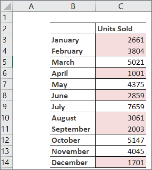
FIGURE 16.1 The cells in this table are conditionally formatted to show a red background for values less than 4000.
To build this basic formatting rule, follow these steps:
- Select the data cells in your target range (cells
C3:C14in this example). - Click the Home tab of the Excel Ribbon and then select Conditional Formatting ➪ New Rule. This will open the New Formatting Rule dialog box, shown in Figure 16.2.
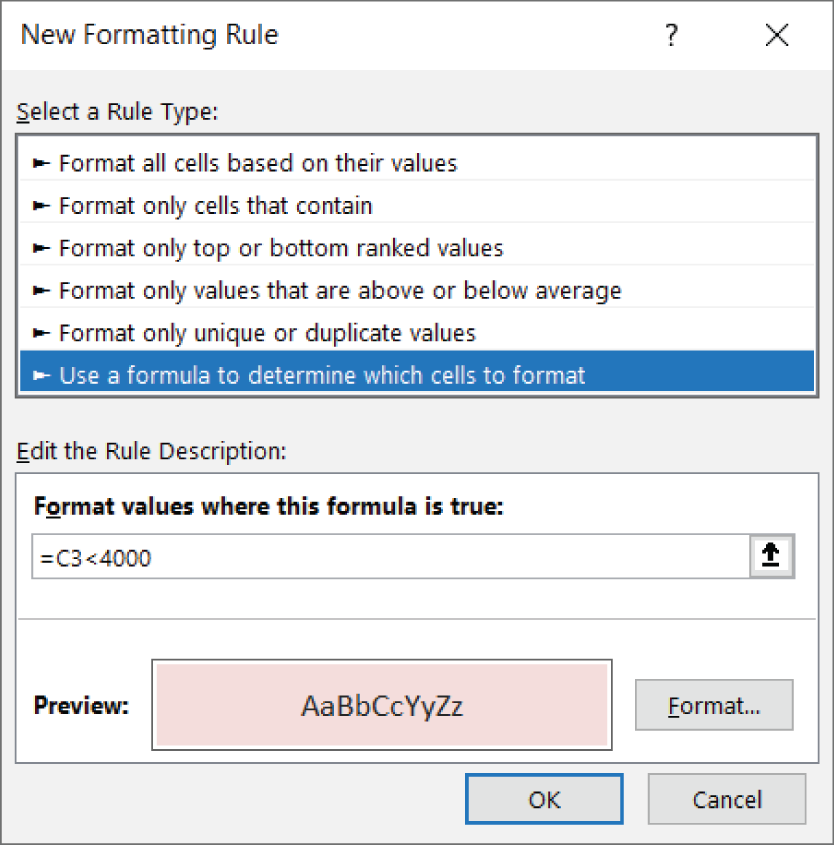
FIGURE 16.2 Configure the New Formatting Rule dialog box to apply the needed formula rule.
- In the list box at the top of the dialog box, click the option called Use a formula to determine which cells to format. This selection evaluates values based on a formula you specify. If a particular value evaluates to
TRUE, then the conditional formatting is applied to that cell. - In the formula input box, enter the formula shown here. Note that we are simply referencing the first cell in our target range. There is no need to reference the entire range.
=C3<4000 - Click the Format button and choose your desired formatting. This will open the Format Cells dialog box where you'll have a full set of options for formatting the font, border, and fill for your target cell.
- Click the OK button once you've completed choosing your formatting options.
- Click the OK button again to confirm your formatting rule in the New Formatting Rule dialog box.
Highlighting cells based on the value of another cell
In many cases, the formatting rule for your cells will be based on how they compare to the value of another cell. Take the example illustrated in Figure 16.3. Here the cells are conditionally highlighted if their respective values fall below the Prior Year Average value shown in cell B3.
To build this basic formatting rule, follow these steps:
- Select the data cells in your target range (cells
E3:E14in this example). - Click the Home tab of the Excel Ribbon and then select Conditional Formatting ➪ New Rule. This will open the New Formatting Rule dialog box shown in Figure 16.4.
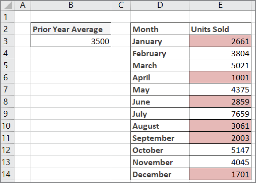
FIGURE 16.3 The cells in this table are conditionally formatted to show a red background for values falling below the Prior Year Average value.
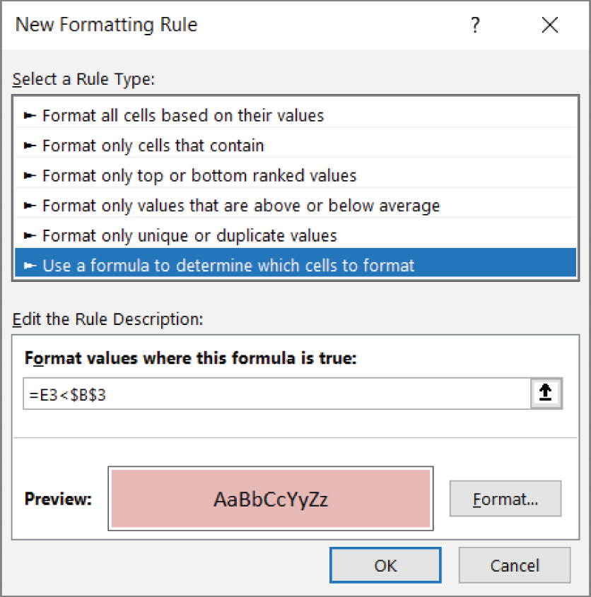
FIGURE 16.4 Compare our target cell (E3) with the value in the comparison cell ($B$3).
- In the list box at the top of the dialog box, click the option called Use a formula to determine which cells to format. This selection evaluates values based on a formula you specify. If a particular value evaluates to
TRUE, then the conditional formatting is applied to that cell. - In the formula input box, enter the formula shown here. Note that we are simply comparing our target cell (E3) with the value in the comparison cell ($B$3). As with standard formulas, you'll need to ensure that you use absolute references so that each value in your range is compared to the appropriate comparison cell.
=E3<$B$3 - Click the Format button and choose your desired formatting. This will open the Format Cells dialog box, where you'll have a full set of options for formatting the font, border, and fill for your target cell.
- Click the OK button once you've completed choosing your formatting options.
- Click the OK button again to confirm your formatting rule in the New Formatting Rule dialog box.
Highlighting Values That Exist in List1 but Not List2
You'll often be asked to compare two lists and pick out the values that are in one list but not the other. Conditional formatting is an ideal way to present your findings. Figure 16.5 illustrates a conditional formatting exercise that compares customers from 2020 and 2021, highlighting those customers in 2021 that are new customers, that is, those customers who did not exist in 2020.
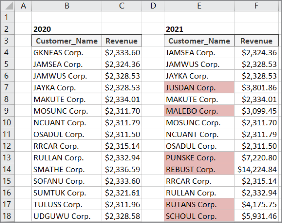
FIGURE 16.5 You can conditionally format the values that exist in one list but not the other.
To build this basic formatting rule, follow these steps:
- Select the data cells in your target range (cells
E4:E28in this example). - Click the Home tab of the Excel Ribbon and then select Conditional Formatting ➪ New Rule. This will open the New Formatting Rule dialog box shown in Figure 16.6.
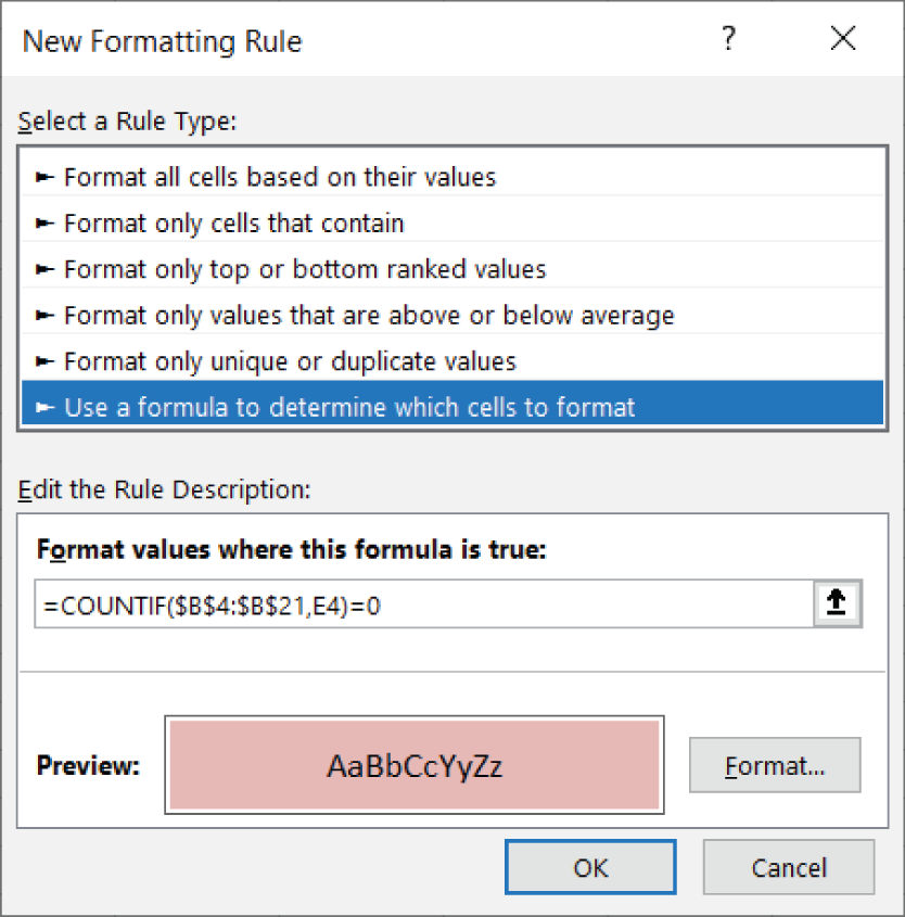
FIGURE 16.6 Apply the conditional format if there are zero instances of the value in the target cell (E4) found in our comparison range ($B$4:$B$21).
- In the list box at the top of the dialog box, click the option called Use a formula to determine which cells to format. This selection evaluates values based on a formula you specify. If a particular value evaluates to
TRUE, then the conditional formatting is applied to that cell. - In the formula input box, enter the formula shown here. Note we're using the
COUNTIFfunction to evaluate whether the value in the target cell (E4) is found in our comparison range($B$4:$B$21). If the value is not found, theCOUNTIFfunction will return a 0, thus triggering the conditional formatting. As with standard formulas, you'll need to ensure that you use absolute references so that each value in your range is compared to the appropriate comparison cell.=COUNTIF($B$4:$B$21,E4)=0 - Click the Format button and choose your desired formatting. This will open the Format Cells dialog box, where you'll have a full set of options for formatting the font, border, and fill for your target cell.
- Click the OK button once you've completed choosing your formatting options.
- Click the OK button again to confirm your formatting rule in the New Formatting Rule dialog box.
Highlighting Values That Exist in List1 and List2
Sometimes, you'll need to compare two lists and pick out only the values that exist in both lists. Again, conditional formatting is an ideal way to present your findings. Figure 16.7 illustrates a conditional formatting exercise that compares customers from 2020 and 2021, highlighting those customers in 2021 who are in both lists.
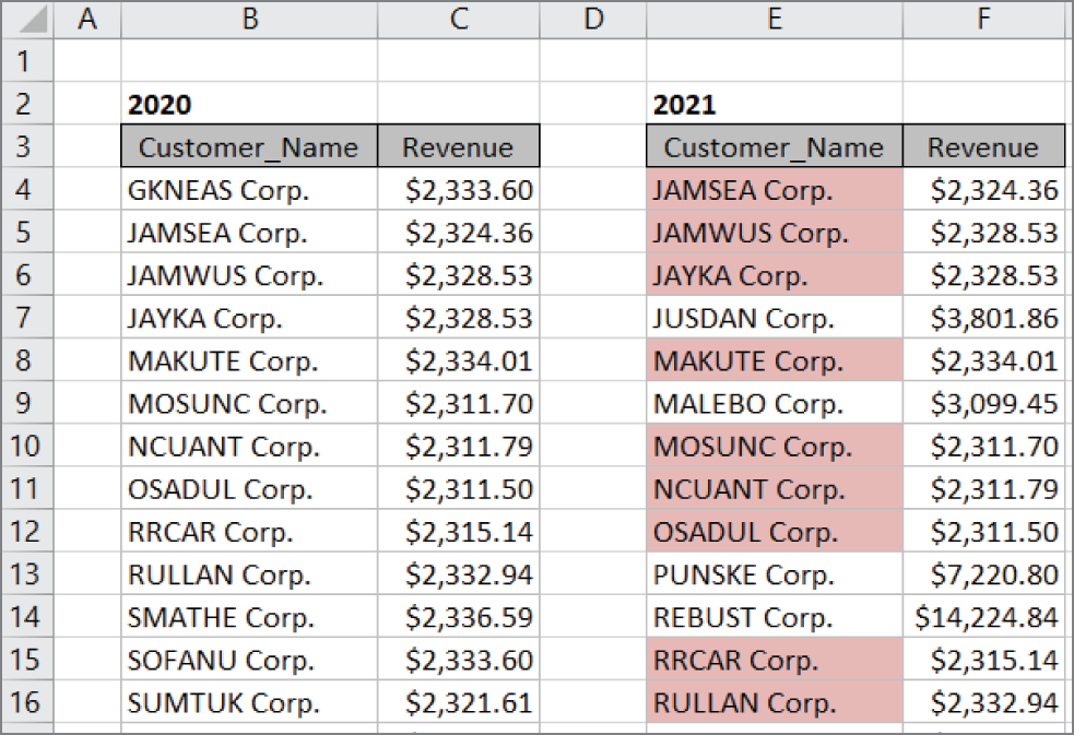
FIGURE 16.7 You can conditionally format the values that exist in both lists.
To build this basic formatting rule, follow these steps:
- Select the data cells in your target range (cells
E4:E28in this example). - Click the Home tab of the Excel Ribbon and then select Conditional Formatting ➪ New Rule. This will open the New Formatting Rule dialog box shown in Figure 16.8.
- In the list box at the top of the dialog box, click the option called Use a formula to determine which cells to format. This selection evaluates values based on a formula you specify. If a particular value evaluates to
TRUE, then the conditional formatting is applied to that cell.
FIGURE 16.8 Apply the conditional format if there is at least one instance (>0) of the value in the target cell (E4) found in our comparison range ($B$4:$B$21).
- In the formula input box, enter the formula shown here. Note we're using the
COUNTIFfunction to evaluate whether the value in the target cell (E4) is found in our comparison range($B$4:$B$21). If the value is found, theCOUNTIFfunction will return a number greater than 0, thus triggering the conditional formatting. As with standard formulas, you'll need to ensure that you use absolute references so that each value in your range is compared to the appropriate comparison cell.=COUNTIF($B$4:$B$21,E4)>0 - Click the Format button and choose your desired formatting. This will open the Format Cells dialog box, where you'll have a full set of options for formatting the font, border, and fill for your target cell.
- Click the OK button once you've completed choosing your formatting options.
- Click the OK button again to confirm your formatting rule in the New Formatting Rule dialog box.
Highlighting Based on Dates
You may find it useful to indicate visually when certain dates trigger a certain scenario. For instance, when working with timecards and scheduling, it is often beneficial to be able to easily pinpoint any dates that fall on weekends. The conditional formatting rule illustrated in Figure 16.9 highlights all of the weekend dates in the list of values.

FIGURE 16.9 You can conditionally format any weekend dates in a list of dates.
To build this basic formatting rule, follow these steps:
- Select the data cells in your target range (cells
B3:B18in this example). - Click the Home tab of the Excel Ribbon and then select Conditional Formatting ➪ New Rule. This will open the New Formatting Rule dialog box, shown in Figure 16.10.
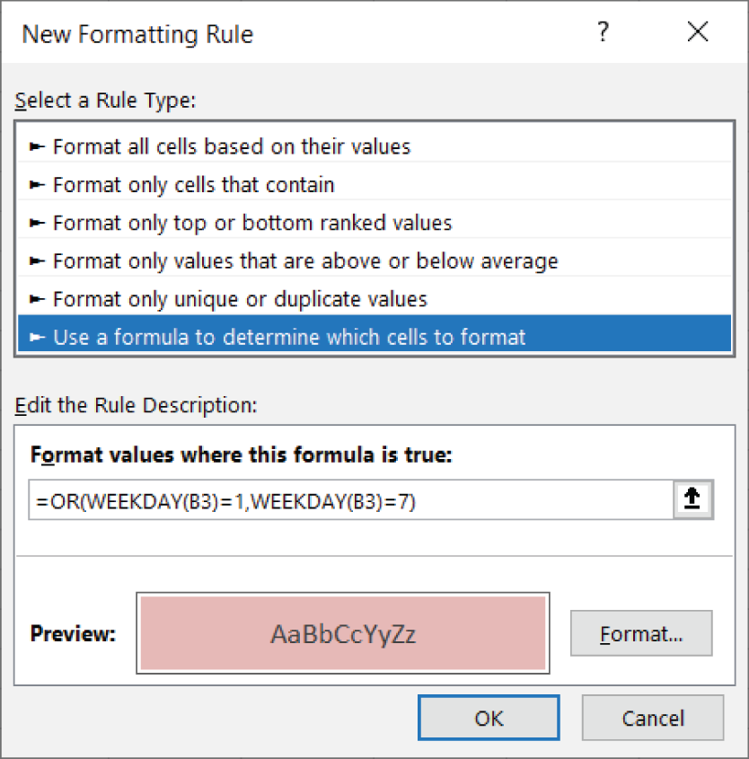
FIGURE 16.10 Using the
WEEKDAYfunction to evaluate the weekday number of the target cell (B3) - In the list box at the top of the dialog box, click the option called Use a formula to determine which cells to format. This selection evaluates values based on a formula you specify. If a particular value evaluates to
TRUE, then the conditional formatting is applied to that cell. - In the formula input box, enter the formula shown here. Note we're using the
WEEKDAYfunction to evaluate the weekday number of the target cell (B3). If the target cell returns as weekday 1 or 7, it means that the date in B3 is a weekend date. In this case, the conditional formatting will be applied.=OR(WEEKDAY(B3)=1,WEEKDAY(B3)=7) - Click the Format button and choose your desired formatting. This will open the Format Cells dialog box, where you'll have a full set of options for formatting the font, border, and fill for your target cell.
- Click the OK button once you've completed choosing your formatting options.
- Click the OK button again to confirm your formatting rule in the New Formatting Rule dialog box.
Highlighting days between two dates
Some analysis requires the identification of dates that fall within a certain time period. Figure 16.11 demonstrates how you can apply conditional formatting that highlights dates based on a start date and end date. As the start and end dates are adjusted, the conditional formatting adjusts with them.
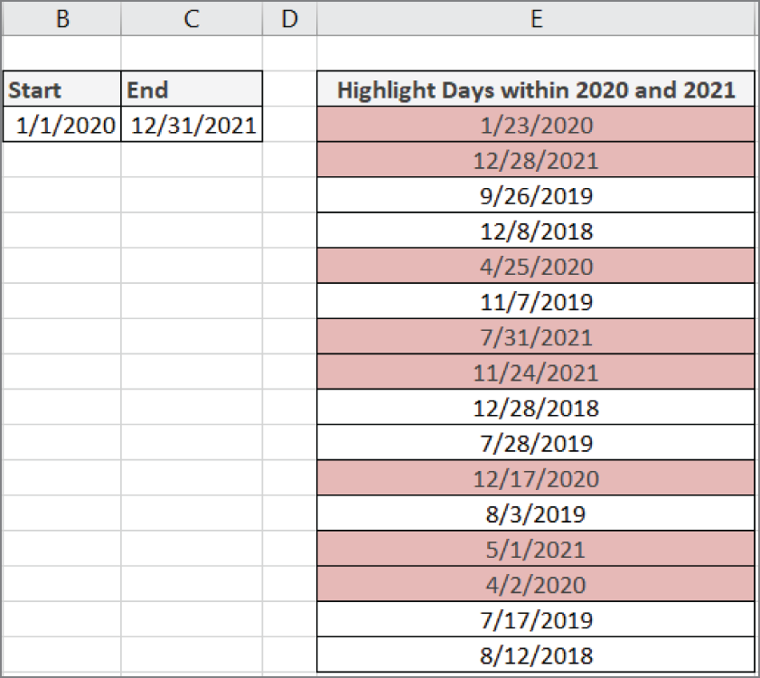
FIGURE 16.11 You can conditionally format dates that fall between a start and end date.
To build this basic formatting rule, follow these steps:
- Select the data cells in your target range (cells
E3:E18in this example), click the Home tab of the Excel Ribbon, and then select Conditional Formatting ➪ New Rule. This will open the New Formatting Rule dialog box shown in Figure 16.12.
FIGURE 16.12 Using the
ANDfunction to compare the date in our target cell (E3) to both the start and end dates found in cells $B$3 and $C$3 - In the list box at the top of the dialog box, click the option called Use a formula to determine which cells to format. This selection evaluates values based on a formula you specify. If a particular value evaluates to
TRUE, then the conditional formatting is applied to that cell. - In the formula input box, enter the formula shown here. Note we're using the
ANDfunction to compare the date in our target cell (E3) to both the start and end dates found in cells $B$3 and $C$3, respectively. If the target cell falls within the start and end dates, the formula will evaluate toTRUE, thus triggering the conditional formatting.=AND(E3>=$B$3,E3<=$C$3) - Click the Format button and choose your desired formatting. This will open the Format Cells dialog box, where you'll have a full set of options for formatting the font, border, and fill for your target cell.
- Click the OK button once you've completed choosing your formatting options.
- Click the OK button again to confirm your formatting rule in the New Formatting Rule dialog box.
Highlighting dates based on a due date
The example shown in Figure 16.13 demonstrates that you can conditionally format dates that are past due by a given number of days. In this scenario, the dates that are over 90 days overdue are highlighted with a red background.

FIGURE 16.13 You can conditionally format dates based on due date.
To build this basic formatting rule, follow these steps:
- Select the data cells in your target range (cells
C4:C9in this example), click the Home tab of the Excel Ribbon, and then select Conditional Formatting ➪ New Rule. This will open the New Formatting Rule dialog box, shown in Figure 16.14.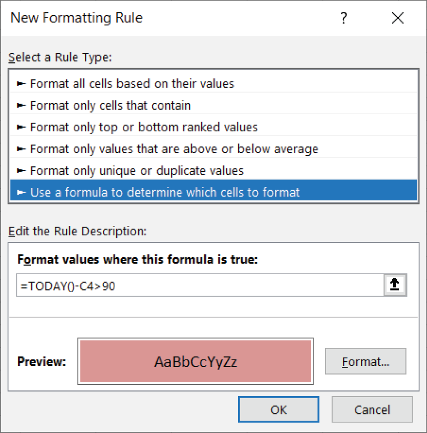
FIGURE 16.14 Evaluating whether today's date is greater than 90 days past the date in our target cell (C4)
- In the list box at the top of the dialog box, click the option called Use a formula to determine which cells to format. This selection evaluates values based on a formula you specify. If a particular value evaluates to
TRUE, then the conditional formatting is applied to that cell. - In the formula input box, enter the formula shown here. In this formula, we're evaluating whether today's date is greater than 90 days past the date in our target cell (C4). If so, the conditional formatting will be applied.
=TODAY()-C4>90 - Click the Format button and choose your desired formatting. This will open the Format Cells dialog box, where you'll have a full set of options for formatting the font, border, and fill for your target cell.
- Click the OK button once you've completed choosing your formatting options.
- Click the OK button again to confirm your formatting rule in the New Formatting Rule dialog box.