
CHAPTER 15
Using Formulas for Matching and Lookups
This chapter discusses various techniques that you can use to look up a value in a range of data. Excel has three worksheet functions (LOOKUP, VLOOKUP, and HLOOKUP) designed for this task, but you may find that these functions don't quite cut it.
In this chapter you'll explore many lookup examples, including alternative techniques that go well beyond the Excel program's normal lookup capabilities.
Introducing Lookup Formulas
A lookup formula returns a value from a table by looking up another related value. A common telephone directory (remember those?) provides a good analogy. If you want to find a person's telephone number, you first locate the name (look it up) and then retrieve the corresponding number.
Several Excel functions are useful when writing formulas to look up information in a table. Table 15.1 describes these functions.
TABLE 15.1 Functions Used in Lookup Formulas
| Function | Description |
|---|---|
CHOOSE
| Returns a specific value from a list of values supplied as arguments. |
HLOOKUP
| Horizontal lookup. Searches for a value in the top row of a table and returns a value in the same column from a row that you specify in the table. |
IF
| Returns one value if a condition you specify is TRUE and returns another value if the condition is FALSE. |
IFERROR
| If the first argument returns an error, the second argument is evaluated and returned. If the first argument does not return an error, then it is evaluated and returned. |
INDEX
| Returns a value (or the reference to a value) from within a table or range. |
LOOKUP
| Returns a value from either a one-row or one-column range. Another form of the LOOKUP function works like VLOOKUP but is restricted to returning a value from the last column of a range. |
MATCH
| Returns the relative position of an item in a range that matches a specified value. |
OFFSET
| Returns a reference to a range that is a specified number of rows and columns from a cell or range of cells. |
VLOOKUP
| Vertical lookup. Searches for a value in the first column of a table and returns a value in the same row from a column that you specify in the table. |
Leveraging Excel's Lookup Functions
Finding data in a list or table is central to many Excel formulas. Excel provides several functions to assist in looking up data vertically, horizontally, left to right, and right to left. By nesting some of these functions, you can write a formula that looks up the correct data even after the layout of your table changes.
Let's take a look at some of the more common ways to utilize Excel's lookup functions.
Looking up an exact value based on a left lookup column
Many tables are arranged so that the key piece of data, the data that makes a certain row unique, is in the far-left column. While Excel has many lookup functions, VLOOKUP was designed for just that situation. Figure 15.1 shows a table of employees. We want to fill out a simplified paystub form by pulling the information from this table when an employee's ID is selected.
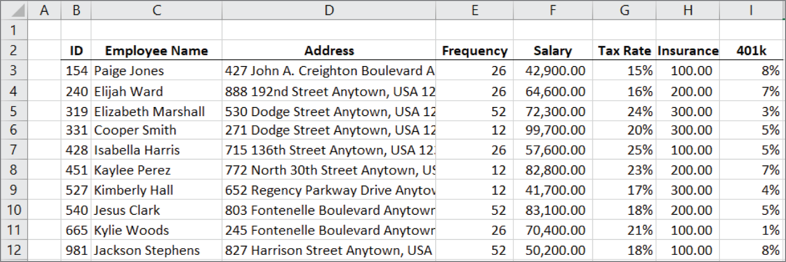
FIGURE 15.1 A table of employee information
The user will select an employee ID from a data validation list in cell L3 (see Figure 15.2). From that piece of data, the employee's name, address, and other information will be pulled into the form. The formulas for the paystub form in Figure 15.2 are shown here:
The formula to retrieve the employee's name uses the VLOOKUP function. VLOOKUP takes four arguments: lookup value, lookup range, column, and match. VLOOKUP will search down the first column of the lookup range until it finds the lookup value. Once the lookup value is found, VLOOKUP returns the value in the column identified by the column argument. In this case, the column argument is 2, and VLOOKUP returns the employee's name from the second column of the lookup range.
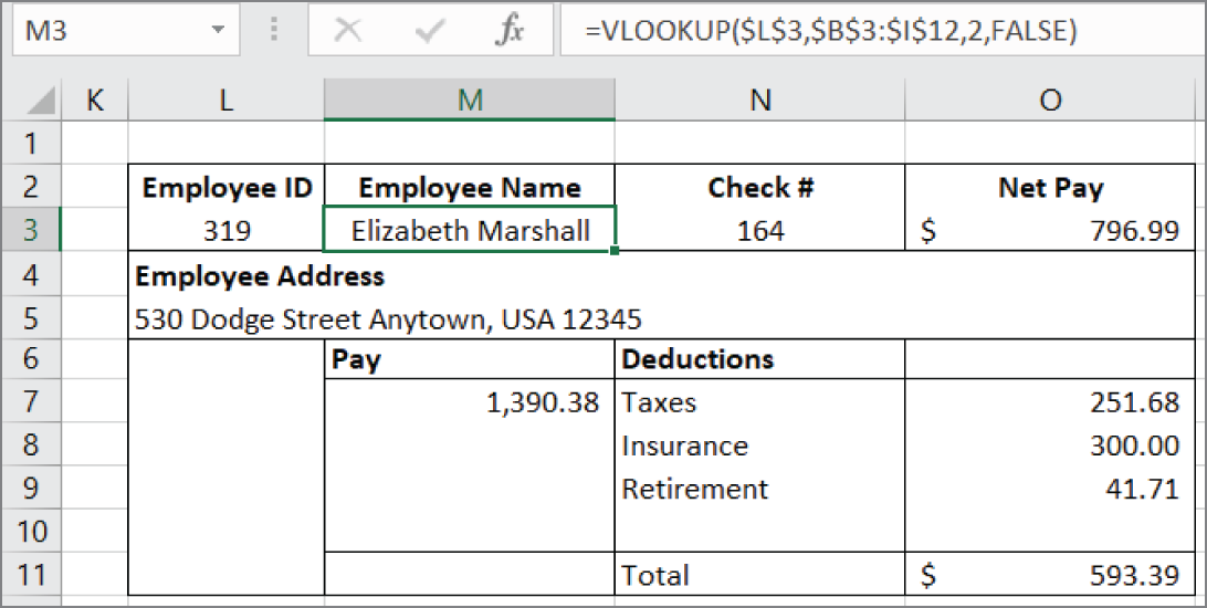
FIGURE 15.2 A simplified paystub form
The other formulas also use VLOOKUP with a few twists. The address and insurance formulas work just like the employee name formula, but they pull from a different column. The pay formula uses two VLOOKUP
s; one is divided by the other. The employee's annual pay is pulled from the fifth column, and that is divided by the frequency from the fourth column, resulting in the pay for one paystub.
The retirement formula pulls the percentage from the eighth column and multiplies that by the gross pay to calculate the deduction. Finally, the taxes formula deducts both insurance and retirement from gross pay and multiplies that by the tax rate, found with VLOOKUP pulling from the sixth column.
Of course, payroll calculations are a little more complex than this, but once you understand how VLOOKUP works, you can build ever more complex models.
Looking up an exact value based on any lookup column
Unlike the table used in Figure 15.1, not all tables have the value that you want to look up in the leftmost column. Fortunately, Excel provides some functions for returning values that are to the right of the value you're looking up.
Figure 15.3 shows the locations of our stores by city and state. We want to return the city and store number when the user selects the state from a drop-down list.
City: =INDEX(B3:D25,MATCH(G4,C3:C25,FALSE),1)Store: =INDEX(B3:D25,MATCH(G4,C3:C25,FALSE),3)
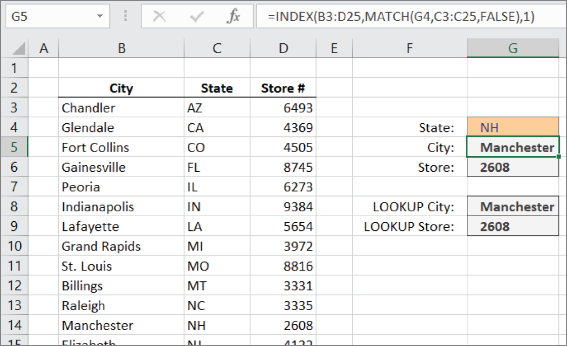
FIGURE 15.3 A list of stores with their city and state locations
The INDEX function returns the value from a particular row and column of a range. In this case, we pass it our table of stores, a row argument in the form of a MATCH function, and a column number. For the City formula, we want the first column, so the column argument is 1. For the Store formula, we want the third column, so the column argument is 3.
Unless the range you use starts in A1, the row and column will not match the row and column in the spreadsheet. They relate to the top-left cell in the range, not the spreadsheet as a whole. A formula like =INDEX(G2:P10,2,2) would return the value in cell H3. The cell H3 is in the second row and the second column of the range G2:P10.
To get the correct row, we use a MATCH function. The MATCH function returns the position in the list in which the lookup value is found. It has three arguments.
- Lookup value: The value we want to find.
- Lookup array: The single column or single row to look in.
- Match type: For exact matches only, set this argument to
FALSEor 0.
The value we want to match is the state in cell G4, and we're looking for it in the range C3:C25, our list of states. MATCH looks down the range until it finds NH. It finds it in the 12th position, so 12 is used by INDEX as the row argument.
With MATCH computed, INDEX now has all it needs to return the right value. It goes to the 12th row of the range and gets the value from either the first column (for City) or the third column (for Store #).
Looking up values horizontally
If the data is structured in such a way that your lookup value is in the top row rather than the first column and you want to look down the rows for data rather than across the columns, Excel has a function just for you.
Figure 15.4 shows a table of cities and their temperatures. The user will select a city from a drop-down box, and you will return the temperature to the cell just below it.
=HLOOKUP(C5,C2:L3,2,FALSE) 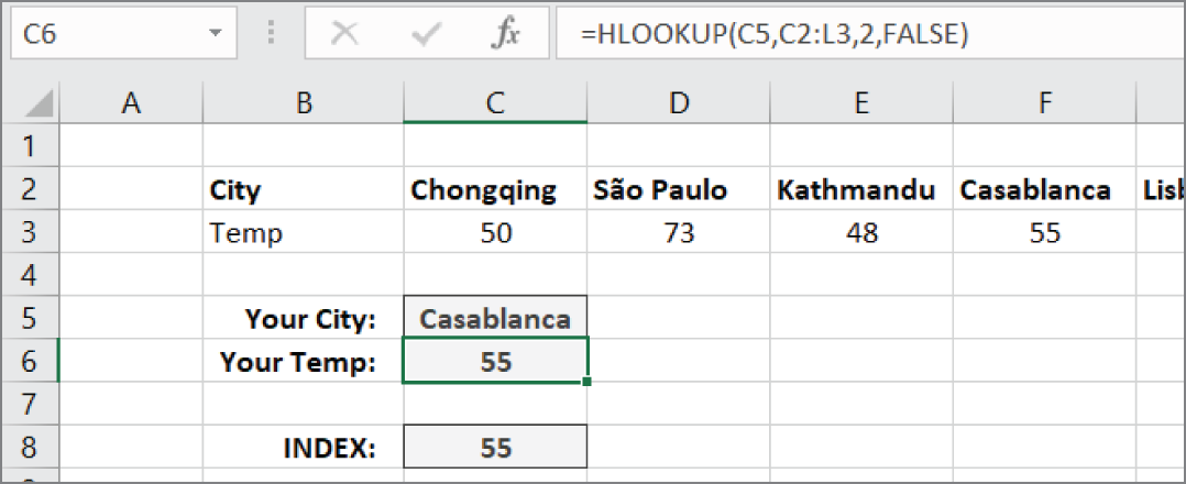
FIGURE 15.4 A table of cities and temperatures
The HLOOKUP function has the same arguments as VLOOKUP. The H in HLOOKUP stands for “horizontal,” while the V in VLOOKUP stands for “vertical.” Instead of looking down the first column for the lookup_value argument, HLOOKUP looks across the first row. When it finds a match, it returns the value from the second row of the matching column.
Hiding errors returned by lookup functions
So far, we've used FALSE for the last argument of our lookup functions so that we return only exact matches. When we force a lookup function to return an exact match and it can't find one, it returns the #N/A error.
The #N/A error is useful in Excel models because it alerts you when a match cannot be found. But you may be using all or a portion of your model for reporting, and #N/A
s are ugly. Excel has functions to see those errors and return something different.
Figure 15.5 shows a list of companies and CEOs. The other list shows CEOs and salaries. A VLOOKUP function is used to combine the two tables. But we obviously don't have salary information for all of the CEOs, so we have a lot of #N/A errors.
=VLOOKUP(C3,$F$3:$G$11,2,FALSE) 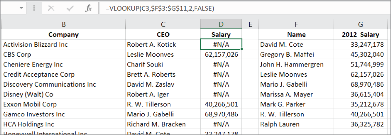
FIGURE 15.5 A report of CEO salaries
In Figure 15.6, the formula has been changed to use the IFERROR function to return a blank if there's no information available.
=IFERROR(VLOOKUP(C3,$F$3:$G$11,2,FALSE),"") The IFERROR function accepts a value or formula for its first argument and an alternate return value for its second argument. When the first argument returns an error, the second argument is returned. When the first argument is not an error, the results of the first argument are returned.
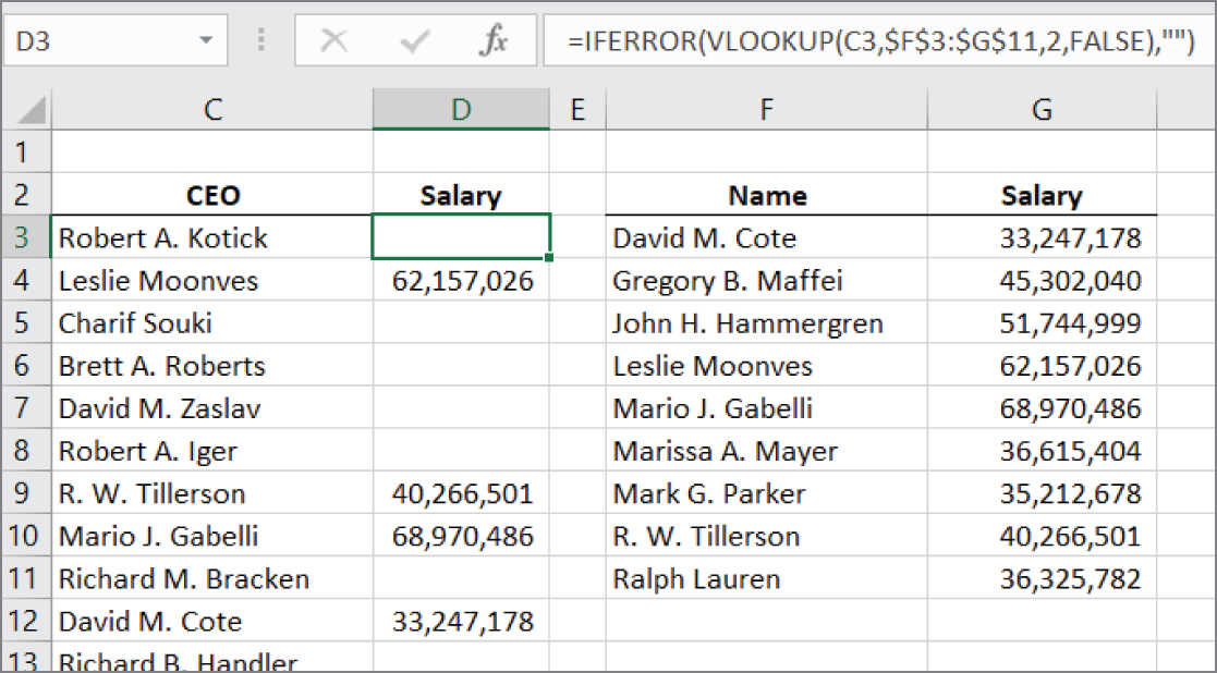
FIGURE 15.6 A cleaner report
In this example, we've made our alternate return value an empty string (two double quotes with nothing between them). That keeps the report nice and clean. But you could return anything you want, such as “No info” or zero.
Finding the closest match from a list of banded values
The VLOOKUP, HLOOKUP, and MATCH functions allow the data to be sorted in any order. Each of them has a final argument that will force the function to find an exact match or return an error if it cannot.
These functions also work on sorted data for the times when you want only an approximate match. Figure 15.7 shows a method for calculating income tax withholding. The withholding table doesn't have every possible value; rather, it has bands of values. You first determine into which band the employee's pay falls, and then you use the information on that row to compute the withholding in cell D16.
=VLOOKUP(D15,B3:E10,3,TRUE)+(D15-VLOOKUP(D15,B3:E10,1,TRUE))*VLOOKUP(D15,B3:E10,4,TRUE) 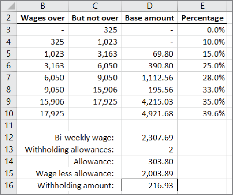
FIGURE 15.7 Computing income tax withholding
The formula uses three VLOOKUP functions to get three pieces of data from the table. The final argument for each VLOOKUP formula is set to TRUE, indicating that we want only an approximate match.
To get a correct result when using a final argument of TRUE, the data in the lookup column (column B in Figure 15.7) must be sorted lowest to highest. VLOOKUP looks down the first column and stops when the next value is higher than the lookup value. In that way, it finds the largest value that is not larger than the lookup value.
In the example in Figure 15.7, VLOOKUP stops at row 5 because 1,023 is the largest value in the list that's not larger than our lookup value of 2,003.89. The three sections of the formula work as follows:
- The first
VLOOKUPreturns the base amount in the third column, or 69.80. - The second
VLOOKUPsubtracts the “Wages over” amount (from the first column) from the total wages. - The last
VLOOKUPreturns the percentage in the fourth column. This percentage is multiplied by the “excess wages,” and the result is added to the base amount.
When all three VLOOKUP functions are evaluated, the formula computes as follows:
=69.80 + (2,003.89 – 1,023.00) * 15.0%Finding the closest match with the INDEX and MATCH functions
As with all of our lookup formulas, the INDEX and MATCH combination can be substituted. Like VLOOKUP and HLOOKUP, MATCH also has a final argument to find approximate matches. MATCH has the added advantage of being able to work with data that is sorted highest to lowest (see Figure 15.8).
The VLOOKUP
-based formula from Figure 15.7 returns #N/A as shown in cell D16 in Figure 15.8. This is because VLOOKUP looks at the middle of the lookup column, determines that it is higher than the lookup value, and then looks only at values before the middle value. Because our data is sorted in descending order, there are no values before the middle value that are lower than the lookup value.
The INDEX and MATCH formula in cell D18 of Figure 15.8 returns the correct result and is shown here:
=INDEX(B3:E10,MATCH(D15,B3:B10,-1)+1,3)+(D15-INDEX(B3:E10,MATCH(D15,B3:B10, −1)+1,1))*INDEX(B3:E10,MATCH(D15,B3:B10,−1)+1,4)
The final argument of MATCH can be −1, 0, or 1.
- −1 is used for data that is sorted highest to lowest. It finds the smallest value in the lookup column that is larger than the lookup value. There is no equivalent method using
VLOOKUPorHLOOKUP. - 0 is used for unsorted data to find the exact match. It is equivalent to setting the final argument of
VLOOKUPorHLOOKUPtoFALSE. - 1 is used for data that is sorted lowest to highest. It finds the largest value in the lookup column that is smaller than the lookup value. It is equivalent to setting the final argument of
VLOOKUPorHLOOKUPtoTRUE.
With a final argument of −1, MATCH finds a value that is larger than the lookup value, and the formula adds 1 to the result to get the proper row.
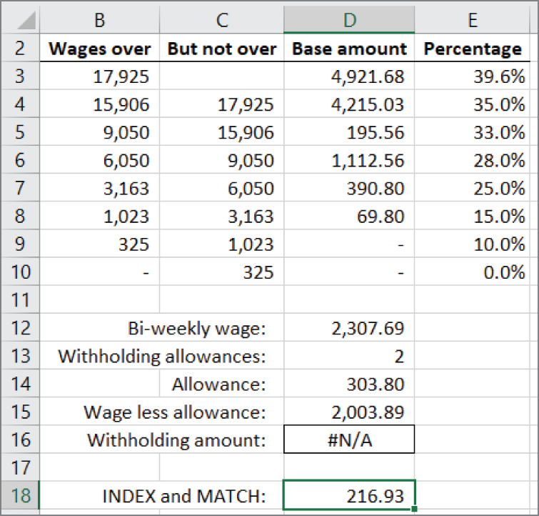
FIGURE 15.8 The same withholding table as Figure 15.7 except the data is sorted in descending order
Looking up values from multiple tables
Sometimes the data that you want to look up can come from more than one table, depending on a choice that the user makes. In Figure 15.9, a withholding calculation similar to Figure 15.7 is shown. The difference is that the user can select whether the employee is single or married. If the user chooses Single, the data is looked up in the single-person table, and if the user chooses Married, the data is looked up in the married table.
In Excel, we can use named ranges and the INDIRECT function to direct our lookup to the appropriate table. Before we can write our formula, we need to name two ranges: Married for the married-person table and Single for the single-person table. Follow these steps to create the named ranges:
- Select the range B4:E11.
- Choose Define Name from the Formulas tab on the Ribbon. The New Name dialog box shown in Figure 15.10 is displayed.
- Change the Name box to Married.
- Click OK.
- Select the range B15:E22.
- Choose Define Name from the Formulas tab on the Ribbon.
- Change the Name box to Single.
- Click OK.
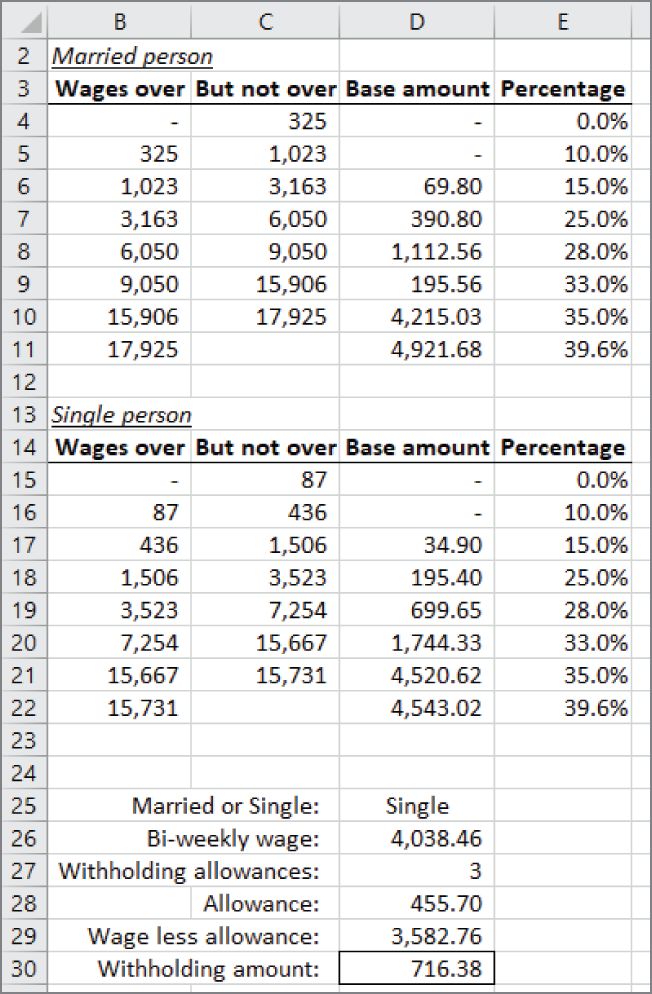
FIGURE 15.9 Computing income tax withholding from two tables
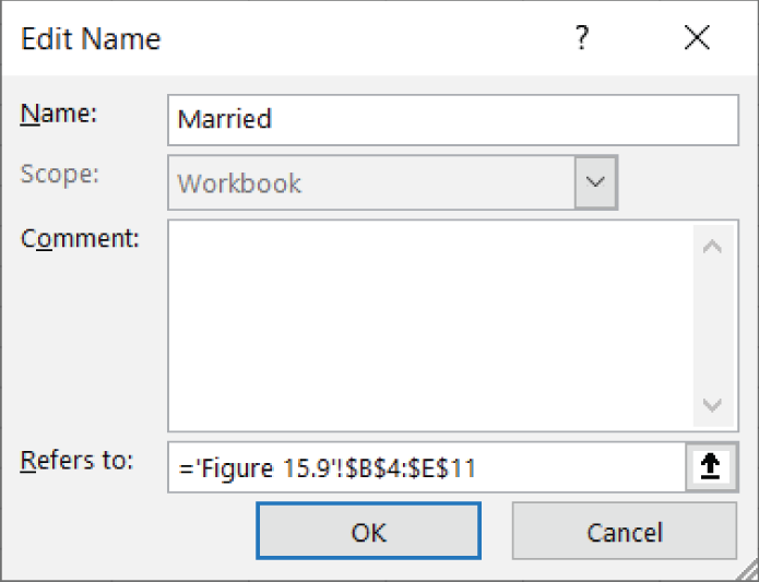
FIGURE 15.10 The New Name dialog box
There is a data validation drop-down in cell D25 in Figure 15.9. The drop-down box contains the terms Married and Single, which are identical to the names that we just created. We'll be using the value in D25 to determine in which table we'll look, so the values must be identical.
The revised formula for computing the withholding follows:
=VLOOKUP(D29,INDIRECT(D25),3,TRUE)+(D29-VLOOKUP(D29,INDIRECT(D25),1, TRUE))*VLOOKUP(D29,INDIRECT(D25),4,TRUE)
The formula in this example is strikingly similar to the one shown in Figure 15.7. The only difference is that an INDIRECT function is used in place of the table's location.
INDIRECT takes an argument named ref_text. The ref_text argument is a text representation of a cell reference or a named range. In Figure 15.9, cell D25 contains the text Single. INDIRECT attempts to convert that into a cell or range reference. If ref_text is not a valid range reference, as in our case, INDIRECT checks the named ranges to see whether there is a match. Had we not already created a range named Single, INDIRECT would return the #REF! error.
INDIRECT has a second optional argument named a1. The a1 argument is TRUE if ref_text is in the A1 style of cell references and FALSE if ref_text is in the R1C1 style of cell references. For named ranges, a1 can be either TRUE or FALSE, and INDIRECT will return the correct range.
Looking up a value based on a two-way matrix
A two-way matrix is a rectangular range of cells. That is, it's a range with more than one row and more than one column. In other formulas, we've used the INDEX and MATCH combination as an alternative to some of the lookup functions. But INDEX and MATCH were made for two-way matrices.
Figure 15.11 shows a table of sales figures by region and year. Each row represents a region, and each column represents a year. We want the user to select a region and a year and return the sales figure at the intersection of that row and column.
=INDEX(C4:F9,MATCH(C13,B4:B9,FALSE),MATCH(C14,C3:F3,FALSE)) By now you're no doubt familiar with INDEX and MATCH. Unlike with other formulas, we're using two MATCH functions within the INDEX function. The second MATCH function returns the column argument of INDEX as opposed to hard-coding a column number.
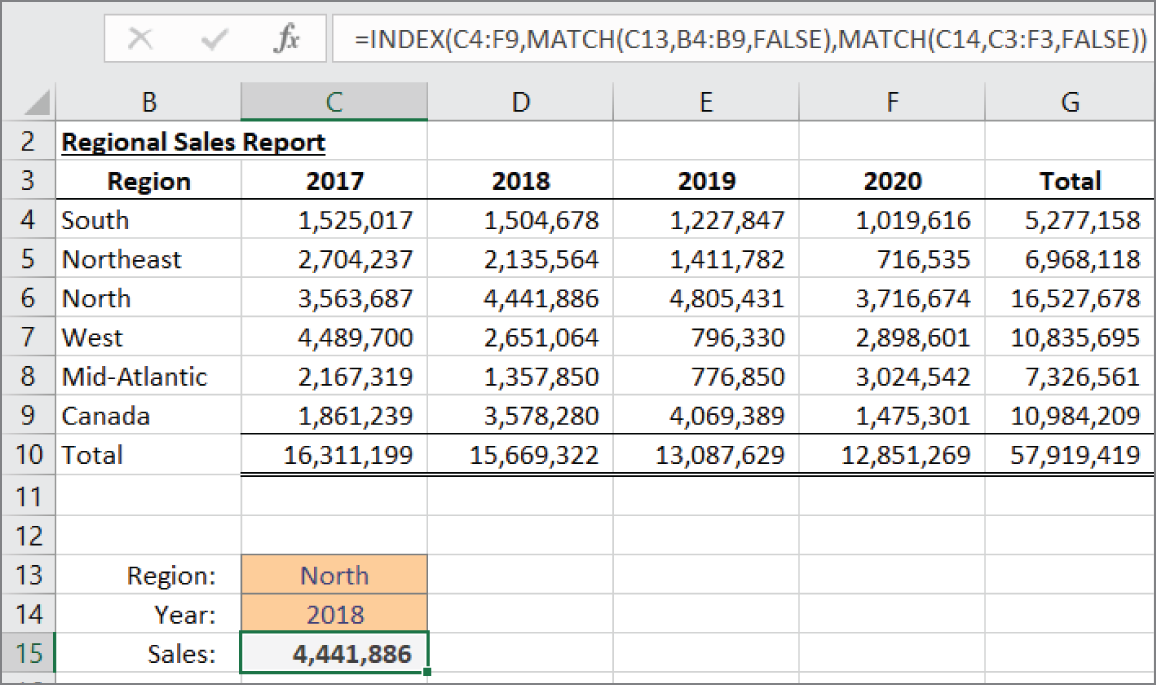
FIGURE 15.11 Sales data by region and year
Recall that MATCH returns the position in a list of the matched value. In Figure 15.11, the North region is matched, so MATCH returns 3 because it's the third item in the list. That becomes the row argument for INDEX. The year is matched across the header row, and since 2018 is the second item, MATCH returns 2. INDEX then takes the 3 and 2 returned by the MATCH functions to return the proper value.
Using default values for match
Let's add a twist to our sales lookup formula. We'll change the formula to allow the user to select only a region, to select only a year, or to select neither. If one of the selections is omitted, we'll assume that the user wants the total. If neither is selected, we'll return the total for the whole table.
=INDEX(C4:G10,IFERROR(MATCH(C13,B4:B10,FALSE),COUNTA(B4:B10)),IFERROR(MATCH(C14,C3:G3, FALSE),COUNTA(C3:G3)))
The overall structure of the formula is the same, but we've changed a few details. The range we're using for INDEX now includes row 10 and column G. Each MATCH function's range is also extended. Finally, both MATCH functions are surrounded by an IFERROR function that will return the Total row or column.
The alternate value for IFERROR is a COUNTA function. COUNTA counts both numbers and text and, in effect, returns the position of the last row or column in our range. We could have hard-coded those values, but if we happen to insert a row or column, COUNTA will adjust to always return the last one.
Figure 15.12 shows the same sales table, but the user has left the Year input blank. Since there are no blanks in the column headers, MATCH returns #N/A. When it encounters that error, IFERROR passes control to the value_if_error argument, and the last column is passed to INDEX.
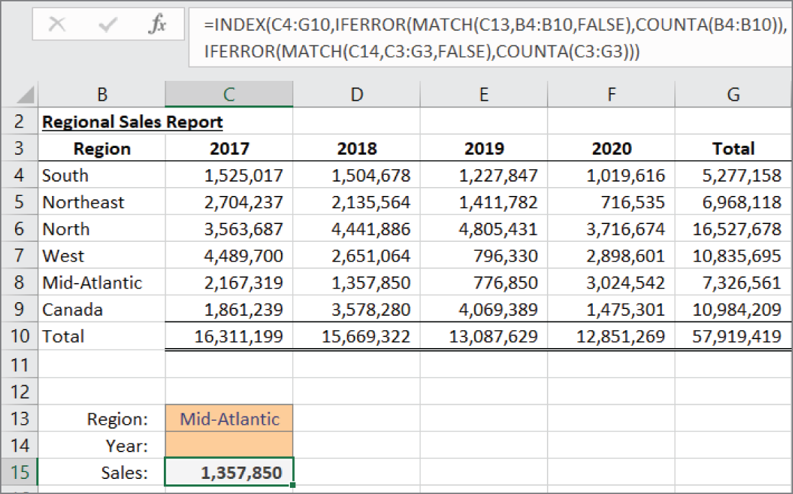
FIGURE 15.12 Returning totals from the sales data
Finding a value based on multiple criteria
Figure 15.13 shows a table of departmental budgets. When the user selects a region and department, we want a formula to return the budget. We can't use VLOOKUP for this formula because it accepts only one lookup value. You need two values because the regions and departments appear multiple times.
You can use the SUMPRODUCT function to get the row that contains both lookup values as follows:
=SUMPRODUCT(($B$3:$B$45=H5)*($C$3:$C$45=H6)*($E$3:$E$45))
SUMPRODUCT compares every cell in a range with a value and returns an array of TRUEs and FALSE
s depending on the result. When multiplied with another array, TRUE becomes 1 and FALSE becomes 0. The third parenthetical section in the SUMPRODUCT function does not contain a comparison because that range contains the value we want to return.
If either the Region comparison or the Department comparison is FALSE, the total for that line will be 0. A FALSE result is converted to zero, and anything times zero is zero. If both Region and Department match, both comparisons return 1. The two 1s are multiplied with the corresponding row in column E, and that's the value returned.
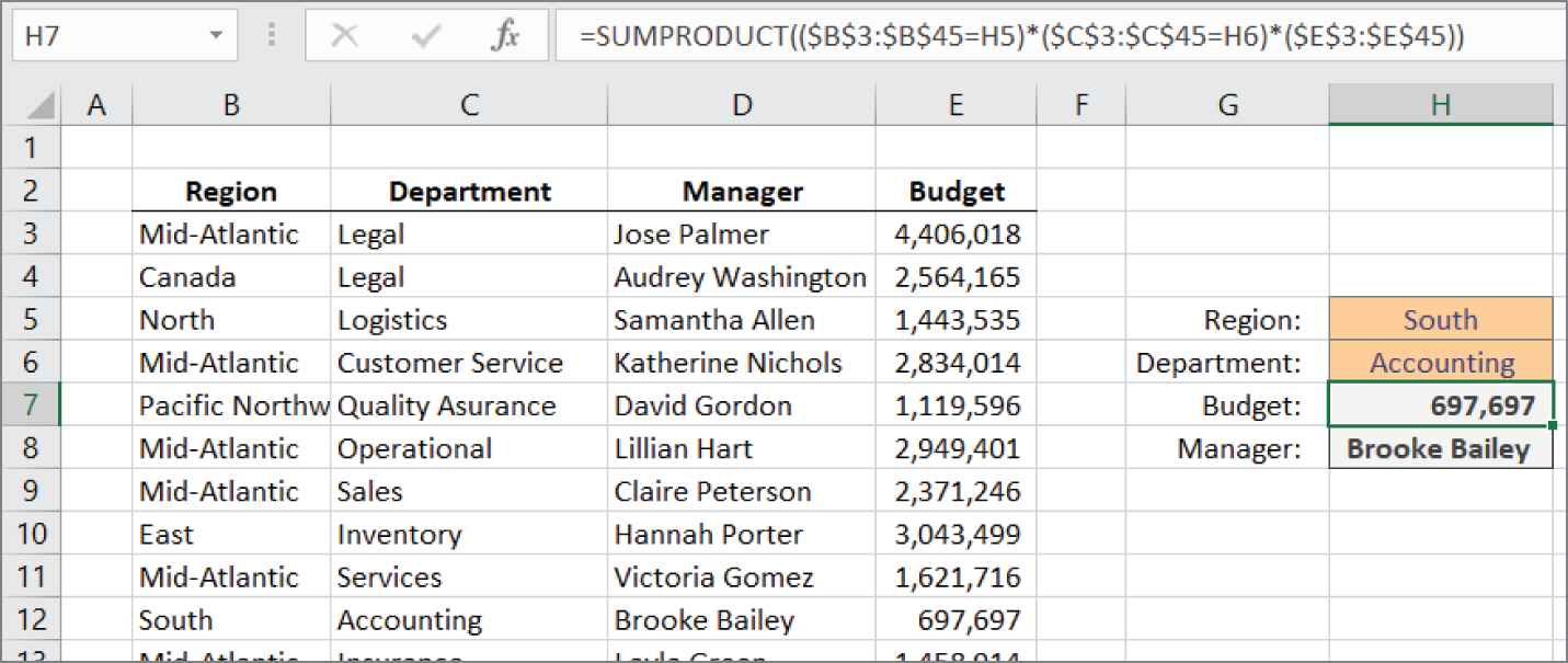
FIGURE 15.13 A table of departmental budgets
In the example shown in Figure 15.13, when SUMPRODUCT gets to row 12, it multiplies 1 * 1 * 697,697. That number is summed with the other rows, all of which are zero because they contain at least one FALSE. The resulting SUM is the value 697,697.
Returning text with SUMPRODUCT
SUMPRODUCT works this way only when we want to return a number. If we want to return text, all of the text values would be treated as zero, and SUMPRODUCT would always return zero.
However, we can pair SUMPRODUCT with the INDEX and ROW functions to return text. If we want to return the manager's name, for example, we could use the following formula:
=INDEX(D:D,SUMPRODUCT(($B$3:$B$45=H5)*($C$3:$C$45=H6)*(ROW($E$3:$E$45))),1)Instead of including the values from column E, the ROW function is used to include the row numbers in the array. SUMPRODUCT now computes 1 * 1 * 12 when it gets to row 12. The 12 is then used for the row argument in INDEX against the entire column D:D. Because the ROW function returns the row in the worksheet and not the row in our table, INDEX uses the whole column as its range.
Finding the last value in a column
Figure 15.14 shows an unsorted list of invoices. We want to find the last invoice in the list. A simple way to find the last item in the column is to use the INDEX function and count the items in the list to determine the last row.
=INDEX(B:B,COUNTA(B:B)+1) 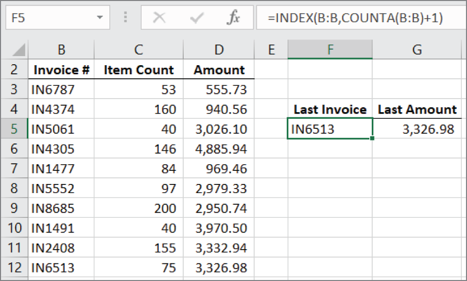
FIGURE 15.14 A list of invoices
The INDEX function when used on a single column needs only a row argument. The third argument indicates the column isn't necessary. COUNTA is used to count the nonblank cells in column B. That count is increased by 1 because we have a blank cell in the first row. The INDEX function returns the 12th row of column B.
Finding the last number using LOOKUP
INDEX and COUNTA are great for finding values when there are no blank cells in the range. If you have blanks and the values you're searching for are numbers, you can use LOOKUP and a really large number. The formula in cell G5 of Figure 15.14 uses this technique.
=LOOKUP(9.99E+307,D:D)The lookup value is the largest number that Excel can handle (just under 1 with 308 zeros behind it). Since LOOKUP won't find a value that large, it stops at the last value it does find, and that's the value returned.
This LOOKUP method has the additional advantage of returning the last number, even if there are text, blanks, or errors in the range.