
6
Topological Study of Electrical Networks
6.1. Introduction
In the face of large numbers of interconnections, electric energy transmission networks are experiencing increasing levels of complexity. For economic reasons, they are often operated close to their operational limit conditions. Most faults, such as cascade tripping or electrical faults, in these systems have serious consequences [TEA 06]. Although any power failure can be attributed to a particular cause (equipment failure, human error, etc.), the electric network should be considered as a complex system and special attention should be paid to its overall behavior, both static and dynamic. This is the main objective of the theory of complex networks [BOC 06]. In this sense, the study of electrical networks has had and is gaining considerable momentum [ALB 04, CAR 02, CRU 05, KIN 05].
Similarly to many systems, an electrical network must face faults which, given its great connectivity, can extend to entire regions: this is known as a blackout (a snow ball effect), that is to say one which has large-scale consequences. The size of electrical networks and their complexity can make it difficult to understand these phenomena which also can emerge locally. With regard to issues such as voltage collapse, network congestion or the blackout phenomenon, the topological complexity of the electrical network is one of the reasons why electrical networks operate within limiting operational conditions. There is a certain number of existing works that are based on the intensive use of statistical physics tools. The adaptation of percolation methods, characteristic degreeless networks and self-organized critical systems are the tools of choice to describe the statistical and topological properties of a network.
The main objective of this chapter is to determine the ability of electrical networks to overcome disruptions or failures (load variations, power lines outage, etc.) through the study of static robustness (namely without taking into account power flows transiting in the network). To this end, we first begin by a “non-comprehensive” study of phenomenological characteristics, or still of observables, which are extracted from the corpus of measures traditionally used for the description of complex networks. We will also study the vulnerability of the network through a study of robustness to attacks and failures. Second, in order to complete this static analysis, we will study the fractality of the network in question by applying three algorithms for the determination of the associated fractal dimension. In addition, we propose a model that may be representative of the dynamics of electrical networks in the last part of the chapter.
6.2. Topological study of networks
Complex systems are a major concern for engineers. For example, electrical networks can be considered as being complex systems with limiting operational conditions where steady increase in electricity demand associated with improving the quality of the network (dimensioning, maintenance, stability, etc.) can become an antagonistic force, leading then to sensitive perturbations. From the analysis of works issued in the scientific literature, different modeling avenues can be put forward, some focusing on the topological nature of the network, others following the direction provided by the dynamics of phenomena involved.
These works, essentially developed in the United States, emerge as the builders of the bridge bringing together the field of statistical physics and the electrical world. Rightly so, we can cite:
- – highly optimized tolerant (HOT) models, introduced by Carlson and Doyle in 1999 [DOY 00, MAN 05, CAR 99], which are intended to model complex and robust systems within an uncertain environment;
- – Dobson et al.’s models [DOB 01, CAR 01] based on stochastic processes whose authors have established close links between self-organized critically systems (SOC) and the electrical network;
- – the structural approaches of the problem making use of graph theory.
In any case, the common denominator of these is the analysis of complexity to better serve it. The first order in this complexity is the existence of scale distributions, thus explaining a dynamic between these different levels of scales through, for instance, the appearance of low power distributions.
6.2.1. Random graphs
The concept of random graphs was introduced for the first time by Erdös and Rényi in 1959 [ERD 59]. Their first approach for the construction of a random graph consisted of establishing a number of links K to be connected and then in randomly selecting two nodes to be connected at each stage of the construction. This type of graph is denoted by ![]() . Another alternative to this approach involves the selection of two nodes and connecting them with probability 0 < p < 1. This type of graph is denoted by
. Another alternative to this approach involves the selection of two nodes and connecting them with probability 0 < p < 1. This type of graph is denoted by ![]() .
.
In the case of small-sized random networks ![]() the distribution of degrees p(k) is a binomial distribution with parameter p unlike large-sized random networks
the distribution of degrees p(k) is a binomial distribution with parameter p unlike large-sized random networks ![]() which have distribution degrees following the Poisson distribution with parameter p(n − 1).
which have distribution degrees following the Poisson distribution with parameter p(n − 1).
In the following, the Erdös and Rényi graphs ![]() and
and ![]() are designated by ER.
are designated by ER.
6.2.2. Generalized random graphs
Despite ER graphs being the most studied models, they are still less representative of real networks. Therefore, it would be interesting to be able to reproduce the characteristics (degree distribution) of a certain type of network.
Random generalized networks allow us to build networks having a degree distribution [BEN 78] p(k) by defining a sequence of integers D = {k1, …, kN} such that 
For the various construction methods of networks with a certain degree distribution p(k), we will refer to Newman et al.’s works [NEW 02, NEW 03].
6.2.3. Small-world networks
One of the most surprising of Milgram’s experiences was to deliver letters to a hundred people whose senders did not know the identity of the recipients and then to assess the number of steps necessary until targeted people received their package. The delivery of someone’s letter to someone else is done in the following way: if the person holding the letter knows the recipient’s identity, it is directly delivered to the latter; otherwise, it is given to another person who has a strong chance of knowing them. Milgram observed that only six steps (on average) are enough to ensure that recipients receive their parcel, hence, the “six degrees” theorem.
This impressive result can be explained by the “small-world” (small diameter) effect of a number of complex networks. Such networks are called “small world”. They are usually characterized by:
- – their small diameter that can be substituted by a small mean of geodesic paths;
- – a large clustering coefficient C.
The Watts and Strogatz (WS) model [WAT 98] is one of the methods generating graphs denoted by ![]() taking into account these two characteristics of small-world networks (small diameter and large clustering coefficient C).
taking into account these two characteristics of small-world networks (small diameter and large clustering coefficient C).
6.2.4. Scale-free networks
Several real networks (Internet networks, protein interaction networks, etc.) have a degree distribution of power distribution of the form P (k) ∼ ck−α. These networks are called scale-free networks and are characterized by the presence of a very small number of nodes of strong degrees. The concept of “scale-free“ comes from power laws that are the only functionals f(x) remaining unchanged (up to a multiplicative factor) after a change of scale.
Barabási-Albert (BA) models [ALB 02] are examples of models that produce scale-free networks. The basic principle for the construction of this kind of networks is that, starting from m0 isolated nodes, we successively add N − m0 nodes having degrees mk ≤ m0, k = 1…N − m0, and which are next connected to an already existing node proportionally to the degree of the latter. Thus, nodes with strong degrees will tend to become more easily connected to a new arriving node. In other words, arriving nodes connect to existing nodes in the graph in a preferential manner.
For more details on the definitions and models previously introduced, the reader can refer to [BOC 06, DOR 08, DOR 03, NEW 03].
6.2.5. Some results inspired by the theory of percolation
In [COH 00, COH 01], a general condition κ is defined, based on the theory of percolation, namely on the fraction of nodes to be removed before a complex network disintegrates (equation [6.1]). It is shown in particular that, in degree distribution networks of power P (k) ∼ ck−α (“scale-free” networks), the fraction pc of nodes to be removed (faults) is expressed according to the connectivity k and quantity fc (equation [6.2]).
This means that for α ≤ 3, the network almost never disintegrates, regardless of the fraction of nodes removed (pc ∼ 0.99 %). As a matter of fact, in this case, κ0 in equation [6.2] converges, proportionally to K, to infinity. Consequently, the quantity 1 − pc in equation [6.1] in turn converges to 0.
It should be recalled that the degree distribution of scale-free networks is given by P (k) ∼ ck−α, designating by k = m, m+1, …, K node connectivity, and m, K, respectively, the minimal and maximal network connectivities. The quantity < kn > designates the n-order moment of variable k.
The general condition for the existence of a large connected component is:

for “scale-free” networks:

In [COH 02], Cohen et al. expressed the percolation threshold by the probability P∞ (equation [6.3)] that a node of connectivity k belongs to the largest connected component that depends of a criticality exponent β, which itself depends on α in the case of scale-free networks (equation [6.5]). On the one hand, results are found again for α ≤ 3 [COH 00] and on the other hand, it is shown that for 3 < α < 4, the criticality exponent β strongly depends on α. Moreover, they have been able to express the mean of connected components < s > after removing a fraction pc of nodes (governed by an exponent γ, equation [6.6]), by equation [6.4]:
by designating q = 1− p (p being the fraction of nodes removed or faulty).
Thus, for “scale-free” networks, the exponents of equations [6.3] and [6.4] can be reduced to:


In [SCH 02], Schwartz et al. have performed the same work as in [COH 02] to express critical exponents β and γ on oriented graphs correlated to the power law (equation [6.8]). They defined a phase diagram that indicates the existence of three states (Figure 6.1) determined by the degree distribution exponent α∗:

designating by αin, αout, respectively, the connectivity of the incoming and outgoing arcs.
They concluded that in this type of network, the critical exponent β is the same as in the case of correlated graphs, by substituting α by α∗:

The study of the diameter of a complex network is one of the most important. In fact, a network becomes effective for energy (or information) transportation when its diameter is small. The small diameter characterizes small-world networks.
In [COH 03], Cohen et al. studied the diameter of random “scale-free” networks and showed that the latter is very small compared to regular random networks:
- – for ER random networks, small-world networks:

- – for “scale-free” networks:

and designating by:
- – d: the network diameter;
- – N: the number of nodes;
- – α: the power law parameter.

Figure 6.1. Phase diagram of the various states in networks oriented and correlated to a power law
In [BRA 03], the authors studied the average length of the optimal paths lopt of ER and WS random networks as well as of small-world networks in the presence of heterogeneities (disorder):
- – in the case of uncorrelated and disorderless networks, the average length of optimal paths is:
- - for the three networks (ER, WS and small-world): lopt ∼ ln N,
- - for “scale-free” networks:

- – in the case of uncorrelated and disorderless networks, the average length of optimal paths is:
- - for ER and WS networks:

- - for “scale-free” networks:

- - for ER and WS networks:
- – in the case of correlated and disordered networks, the average optimal path length is:
- - for “scale-free” networks:

- - for “scale-free” networks:
being the same exponent as in (∗).
In the presence of low heterogeneity, the length of the optimal path is the same as in disorderless networks. In contrast, in the presence of strong heterogeneity, the length of the optimal path lopt is affected by disorder. The same authors [WU 06] have modeled correlations between distribution degrees in a network and have studied the average length of optimal paths of a scale-free network with correlations between distribution degrees. They have concluded that the length of the optimal path lopt increases very significantly in strong heterogeneous networks.
Wang et al. [WAN 08a] have modeled the disorder of a weighted network with a blocking coefficient J:
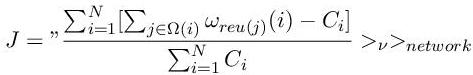
designating by Ω(i) the set of neighbors of the node i:
ωreu(j)(i) is the weight of the link (node i to node j), Ci the total weight coming out of node i, < … >ν is the average under the distribution ν, ν, < … >network is the average under different network configurations.
They show, as in [BRA 03], that blocking (that is disintegration) in a network increases with its heterogeneity. Wang et al. [WAN 08b] studied the robustness of “scale-free” networks by attacking not the nodes of the network, but its links by partitioning the graph in two to find a minimum cut. They concluded that this kind of attack does not necessarily destroy the network and that the latter still remains a “scale-free” network with a very small diameter.
The heterogeneity can be measured by an entropy of the network [FER 03]. In [WAN 06], the authors have showed that maximizing robustness in a “scale-free” network is equivalent to maximizing the entropy of the network degree distribution (equation [6.11]). The entropy of a network is given by the quantity (equation [6.10]):

designating by p(k) the degree distribution of the network and m, the minimal network connectivity.
As a result, it has been shown that the entropy is maximal for exponential networks (the degree distribution of exponential networks is: ![]() .
.
Gallos et al. [GAL 05] have introduced a probability w(ki) (equation [6.12]) that a node with ki links suffers a fault in order to consider the percolation threshold pc when the degrees with highest significance are not known or, in other words, when the attackers do not know the positions of vulnerable nodes in the network:

This modeling provides a means to define a defense strategy against attacks when the costs necessary for the immunization of vulnerable nodes are too high. The authors conclude that a weak knowledge of the “scale-free” network quickly degrades the latter in the event of an attack (α > 0). On the other hand, little knowledge (scale-free) of the network makes it possible to reduce the propagation of faults when defending (α < = 0) against attacks (propagation of viruses in a social network, for example). Paul et al. [PAU 07] studied the percolation threshold pc of regular random graphs by making use of the METIS graph partitioning algorithm [KAR 98], that is:

where k is the network connectivity and pc is the fraction of nodes removed.
At the percolation threshold pc, the diameter and the size of the largest connected component are, respectively, l ∼ N0,25 and S ∼ N0,4.
They concluded that regular random graphs are difficult to attack, possibly to be immunized, because of their homogeneity.
It has been proven that bimodal degree distribution networks are optimal against attacks and failures separately [TAN 05].
Tanizawa et al. [TAN 05] studied the robustness of random “scale-free” and bimodal degree distribution networks, in particular, after a series of simultaneous attacks. They showed that n successive attacks weaken the network more than n simultaneous attacks because the attackers are informed of vulnerable nodes (degree distribution) after each attack. In addition, they concluded that as in [TAN 05], bimodal distribution networks were robust when facing attacks and successive faults.
Robust graphs are characterized by a fraction r of degree distribution nodes: k2 = (< k > −1+r)/r and the other nodes of degree 1. Bimodal distribution networks are optimal for 0.03 <>< 0.9 if pt/pr ≤ 1, otherwise uniform distribution networks are more robust, designating by pt and pr the fractions of faulty and attacked nodes, respectively.
In [SHA 03], by means of algorithmics, Shargel et al. built a class of networks where “scale-free” and exponential networks are special cases and therefore inherit the benefits of both networks, namely, the robustness to attacks from exponential networks [SOL 08] and robustness to faults from “scale-free” networks [COH 00, COH 01].
The degree distribution of exponential networks is ![]() . The critical threshold pc is given by:
. The critical threshold pc is given by: ![]() .
.
In summary, due to their low global connectivity (mean degree) and their small diameter, so-called small-world networks and “scale-free“ networks are effective for routing information (globally and locally). In other words, similarly to purely random networks, small-world graphs are statically robust (resistant to random failure). In contrast, they are more vulnerable to attacks (removal of elements of the highest degree or of more loaded nodes, for instance) [BOC 06, NEW 03, DOR 08]. Similarly, homogeneous networks, such as exponential networks, appear to be more resistant to attacks than heterogeneous networks [WU 08, MOT 02].
6.2.6. Network dynamic robustness
Several models can be found in the literature [CRU 04, KIN 05, CAR 02, WAT 02] destined to reproduce as faithfully as possible the life (or the dynamics) of a network and generally based on an iterative concept. Whether the network is weighted [WU 08, BOC 06, CRU 05, KIN 05] or not [BOC 06], the authors try to define laws for the redistribution of power flows by removing the faulty element (in most of the cases) or by penalizing power flows of faulty elements (for example according to their mean degree and their maximum capacity) [CRU 04, KIN 05]. This study allows, among other things, for the definition of a critical threshold cascade tripping. It is clear that the dynamics of a network strongly depends on its topology.
Rosas-Casas and Corominas-Murtra [ROS 12] in their study of the European electrical network have highlighted this relationship. They have identified three variables that affect the dynamics of a network:
- – the mean degree < k >;
- – the regularity of the distribution of optimal paths in the network;
- – patterns in the graphs (or subgraphs).
In summary, the study of the robustness of a complex network consists of determining the ability of the system to survive disruptions (faults, attacks or load variations in the network). For this purpose, several vulnerability indices have been introduced, of which the most important are the degree distribution of the network (or its connectivity), the network homogeneity, the network diameter and the distribution of geodesic paths within the network, which can be expressed by centrality and betweenness coefficients of nodes or links and patterns (or the subgraphs of the network).
6.3. Topological analysis of the Colombian electrical network
In this section, an arsenal of topological and robustness indicators of electric networks is presented. First of all, we begin by drafting a few observables extracted from the lexicon of graph theory [BER 73] and complex systems [BOC 06, NEW 03] by applying them to the Colombian electrical network. Second, we focus on the study of the robustness and the fractality of the network and in particular, three algorithms will be presented.
6.3.1. Phenomenological characteristics
6.3.1.1. Some topological indicators
Before introducing some definitions (characteristics) of a graph, the latter is defined as follows.
A graph G, often denoted by G = (V, E), is a pair of set (V, E) where V = {v1, …, vN} and E = {e1, …, eK}, respectively, designates the sets of N nodes and K links (i, j) ∈ V2 of the graph G.
The graph G can be described in the form of a matrix in two different manners:
- – adjacency matrix A: this is a square matrix N × N of elements aij (i, j = 1, …, N) where aij = 1 if the node i is adjacent to the node j and 0 otherwise;
- – incidence matrix B: this is a matrix of dimension N × K of elements bik (i = 1, …, N ; k = 1, …, K), where bik = 1 if the node i ∈ V is adjacent to the link k ∈ E and 0 otherwise.
6.3.1.2. Node degree, mean graph degree, homogeneity and correlations
The degree, sometimes referred to as connectivity, of a node i ∈ V denoted by ki is the number of links (i, j) ∈ V2 adjacent to the node i (that is the number of neighbors of i). More formally, ![]() designating by aij the elements of the adjacency matrix A corresponding to the graph G. Thus, the mean degree of the graph G is the first-order moment (expectancy) < k > of the degree distribution P (k):
designating by aij the elements of the adjacency matrix A corresponding to the graph G. Thus, the mean degree of the graph G is the first-order moment (expectancy) < k > of the degree distribution P (k):

When the degree distribution P (k) is not regular, it is said that the graph G is heterogeneous. Otherwise, the graph is known as homogeneous (regular).
The degree distribution p(k) provides us with a representation of the connectivity of the nodes as they are actually connected in the graph. Nonetheless, correlations between node degrees can hide in the graph, that is to say, the probability that a node of degree k becomes connected to another node of degree k′ depends on k. In other words, it is possible that there is a preferential linkage relationship between nodes. The correlations of the degrees of node i, knn,i, can be measured by introducing the mean degree of nearest neighbors of node i, defined as follows:

where ηi and ki, respectively, designates the set of the neighbors of node i and its degree in the graph.
Therefrom, the nearest neighbors mean degree, knn(k), of any node of degree k can be expressed by the quantity [PAS 01]:

in which P (k′|k) designates the conditional probability of a node of degree k′ to become connected to another node of degree k.
When knn(k) is increasing, the correlation is known as being assortative. It is referred to as diassortative, when knn(k) is decreasing. In the absence of correlations, the quantity knn(k) decreases to ![]() that is knn(k) is independent of k.
that is knn(k) is independent of k.
In reality, formula [6.15] is hardly computable. To address this problem, the Pearson correlation coefficient r constitutes another alternative to calculate the quantity knn(k). It is defined as follows [NEW 02]:

designating by ji, ki, respectively, the degrees of both nodes constituting the link i, with i = 1, …, K.
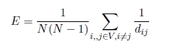
6.3.1.3. Geodesic paths mean, diameter and efficiency
The geodesic path is one of the most important parameters of a graph. In fact, the transmission of information in a graph G necessarily involves the manipulation of the geodesic paths of the latter. Formally, the geodesic path between a node i and a node j, denoted by dij, is the quickest existing path in the graph between the two nodes. The maximal value of all the dij is called the graph diameter (Diam(G)). Therefrom, the mean geodesic path L of a graph G can be defined as follows:

In case the graph G is not connected (that is there are nodes unreachable from other nodes in the graph), the mean geodesic path L and the diameter of the graph diverge. Moreover, the latter are one of the efficiency measures of a network that can be used as network robustness indicators. In order to address this divergence problem, the global efficiency E of the graph G is defined as being the harmonic mean of geodesic paths, namely:
6.3.1.4. Centrality and betweenness coefficient
The nodes centrality and betweenness coefficient (eventually of links) is one of the most widespread characteristics of a graph. In fact, this measure allows us to determine the role or importance of each node (possibly a link) of the graph. Originally, the centrality and betweenness coefficient had been introduced to measure the importance of an individual in social networks [WAS 94]. It is defined as the number of times that a node (link) has appeared in the construction of the geodesic paths of the graph. More specifically, the centrality and betweenness coefficient of a node i, which will be denoted by bi, is defined by the relation [6.19]:

designating by njk, the number of geodesic paths between the node j and node k and njk(i), the number of geodesic paths between nodes j and k, passing through node i.
As an illustration in graph G in Figure 6.2, we have:

Figure 6.2. a) Triangle, b) triplet and c) illustrative graph
6.3.1.5. Clustering coefficient
People usually say “my friend’s friend is my friend”. This expression has nothing banal. As matter of fact, friends of an individual have a strong chance of knowing each other due to their similarity (interests, meeting places, proximity, etc.). This probability of relation between the friends of an individual can be measured by the clustering coefficient or transitivity of the latter. More formally, the clustering coefficient ci of a node i is defined as follows:

designating by ei the maximum number of links in the subgraph of the neighbors of node i.
As an illustration in graph G of Figure 6.2(c), ![]() and
and ![]()
The quantity ci is not a measure common to all nodes of the graph G. As a result, the overall behavior of the latter is difficult to define when using equation [6.20] only. Another quantity called “mean clustering coefficient” of a graph G can then be introduced, which is defined as the mean of all cluster coefficients of the nodes of G:

The formula [6.21] measures the density of triangles that are present in the graph G (Figure 6.2) for the definition of a triangle and a triplet. Consequently, the measure ci can be replaced by transitivity T defined as follows:

The examinations of equations [6.20]–[6.22] brings us to the following comments:
- – 0 ≤ ci ≤ 1, 0 ≤ C ≤ 1;
- – the cluster coefficient of the links can be similarly defined as for the nodes;
- – the cluster coefficient c(k) of a class of nodes of degree k can be defined.
As an illustration in graph G in Figure 6.2(c), we have:

As stated at the beginning of the chapter, this list of indicators is far from being exhaustive. For other characteristics of a graph, we will refer to: [BOC 06, NEW 03, DOR 03, DOR 08].
6.3.1.6. Results
We have focused on the Colombian electrical network. The information available to us concerns the structure of the network, its workload and the history of incidents. In the data provided by the Colombian operator, we can find an a priori comprehensive map of its network and a database of incidents that occurred in the network since 1996. The map comes in the form of a backup file of a case study from the software program DigSilent. This software is a complete environment for the study of Power Flow published by a German company. Moreover, the GPS coordinates of the Colombian network have been provided in the form of a Keyhole Markup Language (KML) file.
To make these raw data usable by our algorithms, it has been necessary to extract them from their software environment (DigSilent). The procedure has consisted of exporting in a proprietary DigSilent format (.dgs ASCII format) the database of the operator and writing Python scripts to read the text file to extract the relevant data. Those of interest to us in this section of the chapter concern the topology (lines, stations and substations) of the network. It has thus been possible to perform the manipulation and the interaction of the results in the form of the KML language (Google Earth) by means of programs developed in Python. An example of a KML file of the resulting Colombian network is presented in Figure 6.3. Despite this Google Earth presentation being more elegant and practical, in the following we will make use of a module in the graph processing library in Python for visualization purposes: NetworkX.
Once a workable version of the Colombian network has been obtained, we have compiled the set of codes related with the characterization of graphs to make a coherent and comprehensive application, capable of executing all the processes in a target graph. This program has been named BTGT. It comprises a main kernel, including processing unit modules and a graph manager.

Figure 6.3. Colombian network (500 kV and 220 kV lines) in KML file format (Google Earth). For a color version of this figure, see www.iste.co.uk/heliodore/metaheuristics.zip
It has been designed in a modular to allow, via the Python legacy, the addition of future modules. The integrated modules are the modules for the computation of betweennesses, clustering indices and degree distributions. Subsequently, attack and fault vulnerability tests as well as a module for the computation of the fractal dimension of graphs have been added. Moreover, the Python program BTGT implemented generates a text file containing the main phenomenological characteristics of a network.
An example of a file obtained using the program applied to the Colombian network is outlined as follows:


Figure 6.4. Results with the Colombian network: a) link centrality coefficient (betweennesses); b) knot centrality coefficient; c) clustering coefficient (clustering); d) center and periphery
The results obtained with the Colombian network are represented in Figures 6.4 and 6.5. Figures 6.4(a)–(c), (e) and (f), respectively, represent the links and the nodes centrality coefficients, the nodes clustering coefficients, the degree distribution in linear evolution and in loglog diagram of the Colombian electrical network.
The attenuated colors of the nodes or links in Figures 6.4(a)–(c), respectively, indicate that they are small centrality or clustering coefficients. In contrast, the nodes or links of larger coefficients are represented with darker colors.
In Figure 6.4(d), nodes having a square scheme represent the center of the network, those with a triangular scheme represent its periphery and darker colors indicate distance from the center network nodes. Conversely, nodes close to the center are represented by faded colors.

Figure 6.5. Results with the Colombian network: a) degree distribution; b) degree distribution in a loglog diagram
After examination of these curves, the following comments can be made:
- – the Colombian network is not locally efficient. In fact, clustering indices indicate the local efficiency of the network. In other words, if a node with a high clustering index (dark color) suffers a fault, its strong connectivity makes it possible to bring the energy through its nearest neighbors. Figure 6.4(d) clearly shows that there are few regions with a high clustering coefficient;
- – the Colombian network can be considered as scale free, with as exponent: γ =3.26. Furthermore, Figure 6.4(f) shows a linear behavior in the loglog diagram of the degree distribution of the Colombian network. Moreover, the network cannot be considered as being small world. As a matter of fact, the diameter and the mean geodesic path of the network are too large to be considered as such;
- – the negative value of the Pearson correlation coefficient r suggests that the Colombian network is disassortative. In other words, preferential linkages are possible in the network.
6.3.2. Fractal dimension
The fractal dimension, denoted by D, is a quantity that gives an indication of how a fractal set fills the space. There are many definitions of the fractal dimension [THE 90]. The most important fractal dimensions encountered in the literature and formally defined are the Rényi dimension and the Hausdorff dimension.
Fractal dimensions are used in many research areas such as physics [ZHA 10], image processing [SOI 96, TOL 03], acoustics [EFT 04] and chemistry [EFT 04]. In addition to formal and theoretical aspects, many organizations and phenomena of the real world exhibit fractal properties (vegetation, cellular organisms, seismicity, etc.), namely self-similarity properties (deterministic or stochastic).
For this chapter, the need to be able to dispose of the estimation of the fractal dimension is what we will recall from this chapter because phenomena involved in the dynamics of electric networks suggest scale properties:
- – scale properties at the level of the electrical network graph, knowing that the definition of the fractal dimension of graphs is carried out by extension, the concept of metric is hardly apprehensible [TAN 05, THE 90, SON 07];
- – scale properties in the dynamics itself of these networks, from the moment the self-organized criticality model becomes relevant to them [CAR 02]. The object in question is a time series or a set of sampled data.
Concerning the estimation of graphs fractal dimensions, we present three of the most used algorithms namely:
- – the graph coloring (GC) algorithm;
- – the Compact–Box–Burning (CBB) algorithm;
- – the Maximum-Excluded-Mass-Burning (MEMB) algorithm.
The benefit of the description of these algorithms is directly connected to the study of random walks in a graph, the emergence of faults in a node, eventually a link, and the topology of the graph. In other words, it would be interesting to detect self-similarity properties governing the graph (failure, random walk in the graph, topology of the graph, etc.).
Before presenting these methods, it is necessary to formally define what is a “box” and what is a “fractal” dimension:
DEFINITION 6.1.– In a graph G = (V, E), we call a box of size lB (respectively, of radios rB), a subgraph H = (V ′, E′) of G such that ∇(i, j) ∈ V′2, lij < lB (respectively, lij ≤ 2 ∗ rB).
DEFINITION 6.2.– Let K be a compact subset of ![]() Nε(K) designates the minimum number of closed balls of radius ε necessary to cover K. The fractal dimension is then defined (if it exists), denoted Df, by:
Nε(K) designates the minimum number of closed balls of radius ε necessary to cover K. The fractal dimension is then defined (if it exists), denoted Df, by:

Referring to definition 6.2, the fractal dimension of the compact subset K then corresponds to the slope in the loglog diagram of Nε(K) and ![]()
Despite the fact that in the field of mathematics the notion of fractal dimension is very specific, it remains, however, less obvious regarding its definition in a graph. In effect, we can define as many metrics as we wish in a graph. In the following and referring to definitions 6.1 and 6.2, we define a fractal dimension of graph G = (V, E) in two ways [COS 07]:
- – the first, originating from the box method, covers the network with NB boxes with a side (diameter) ℓB, that is the distance between two nodes in a box is less or equal to ℓB. By denoting the fractal dimension by dB, a fractal graph will then follow the law [6.24]:
- – the second, issued from the Cluster Growing method, randomly chooses a seed node and forms a cluster from this node, that it to say, it takes all available nodes within a distance less than or equal to ℓ, then resumes operation until exhaustion of available nodes. Denoting by Mc the mean mass of the set of resulting clusters and the fractal dimension of the associated graph dC, a fractal graph will then follow the law [6.25]:
Despite the fact that these two definitions are exclusive in some cases, that is, there are situations where a graph is fractal following only one of these two definitions, these cases are, nonetheless, still rare. Subsequently, the first definition will be preferred because it is more consensual in the literature.
6.3.2.1. The GC algorithm
In [SON 07], it has been found that the problem of the optimal coverage of a graph G employing boxes with maximal size lB is tantamount to solving the coloring problem of the associated dual graph G′. Starting from the initial graph G and by setting the boxes maximal size to lB, two nodes i and j of the graph G′ are connected if they are separated by a geodesic distance, in the original graph G, lij ≥ lB. In Figure 6.6(a), nodes 2, 3 and 8 are, relatively to node 1, at a distance less than or equal to 3. Therefore, they cannot be connected to node 1 in the dual graph G′ (Figure 6.6(b)).
Algorithm 6.1: Greedy coloring, GC
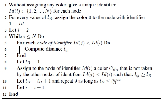
The algorithm proposed in [SON 07] utilizes a conventional constructive coloring method called (Greedy) and at the same time builds the dual graph G′. The general operating principle of the approach is described in algorithm [6.1].
It first starts by the indexation of the nodes, next the color 0 is assigned to the node of identifier Id = 1 and continues for all the values of lB. In effect, each node of the graph will have as many colors as the number of variations of lB. As an example, if lB takes its values within {1,2,…,M}, each node will consequently have M colors. At each iteration i, the calculation of distances lij are only performed for nodes j of identifier Id(j) < Id(i). At the end of the algorithm, the fractal dimension of the graph is identified as the slope in the loglog diagram of the number of boxes needed to cover the whole of the graph according to the maximal size of the latter (that is lB).

Figure 6.6. Example of the application of the coloring algorithm, lB = 3 : a) the initial graph G; b) the dual graph G′; c) solution of the coloring problem of the dual graph G′; d) the final result (number of boxes NB = 2). For a color version of this figure, see www.iste.co.uk/heliodore/metaheuristics.zip
6.3.2.2. The CBB algorithm
The general operating principle of the CBB algorithm is outlined as follows:
- – first, all nodes are likely to be selected to belong to the current box. A node p is randomly selected in the graph (Figure 6.7(a)), this node represents the center of the box under consideration (the nodes in black in Figure 6.7);
- – next, all nodes i of the graph (nodes in red in Figure 6.7) that are at a geodesic distance lip ≥ lB are set aside;
- – the selection process is reiterated for a new center of the box in the subgraph resulting from every selection stage until none of the node is likely to belong to the box (Figures 6.7(b) and (c));
- – at the end of these steps, a box is built containing nodes at geodesic distance at most lB − 1 (Figure 6.7(c));
- – lastly, the procedure for the construction of the boxes is repeated until all nodes are assigned to a box (Figures 6.7(d)–(f) for iteration 2, Figure 6.7(g)–(i) for iteration 3, Figure 6.7(j) for iteration 4).
The summary of the CBB technique is presented in algorithm 6.2.
Algorithm 6.2: Compact–Box–Burning, CBB

6.3.2.3. The MEMB algorithm
The MEMB algorithm aims to improve the randomness aspect in the selection of the central nodes of the boxes of the CBB algorithm. The concept of the algorithm is based on the choice of hubs (nodes with stronger degree) as boxes centers, which a priori brings us closer to the optimal solution.
To this end, we first define the notion of “excluded mass” as follows:
- – for a given covering radius rB, the “excluded mass” of a node i is equal to the number of nodes j (including the node i in question) that are at geodesic distance lij ≤ rB and which are not yet assigned to a box (visited). In Figure 6.8(a), node 3 includes three nodes that are at geodesic less than rB = 1, its ”excluded mass” is thus equal to 4;
- – it then simply suffices to calculate the “excluded masses” of all the non-central nodes at every stage of the algorithm and choose the node p of the most significant “excluded mass” as the new center of the new box and then mark all the nodes i at geodesic distance ljp ≤ rB as being “marked”.
The summary of the MEMB technique is presented in algorithm 6.3 and Figure 6.8 illustrates the application of the MEMB algorithm when rB = 1.

Figure 6.7. Application example of the CBB algorithm, lB = 2: nodes in red correspond to nodes “set aside” (geodesic distance ≥ lB), in black to “central” nodes, in green to nodes that are at geodesic < lB. a) Random selection of node 3 and removal of nodes at a distance ≥ lB from node 3. b) Random selection of node 4 and removal of nodes at distance ≥ lB from node 2. c) Selection of the remaining node 5. Iteration 1: (a)–(c). Iteration 2: d)–f). Iteration 3: g)–i). Iteration 4: j). (d) The final result (number of boxes NB =4). For a color version of this figure, see www.iste.co.uk/heliodore/metaheuristics.zip
Algorithm 6.3: Maximum–Excluded–Mass–Burning, MEMB


Figure 6.8. Application example of the MEMB algorithm, rB = 1: nodes in green correspond to “unmarked” nodes, in yellow to “marked nodes” and black nodes to “central nodes”. The gray nodes are nodes that already belong to a box. (a)–(c) Intermediate results of the MEMB algorithm; (d) final result (number of boxes NB = 2 = number of hubs). For a color version of this figure, see www.iste.co.uk/heliodore/metaheuristics.zip
6.3.2.4. Results
Figures 6.9(a)–(c), respectively, represent the results obtained when applying algorithms GC, CBB and MEMB to the IEEE 57-node, 118-node and 300-node networks benchmarks.
On the other hand, Figures 6.10(a) and (b) represent the comparison of fractal dimensions obtained by the application of the three algorithms to the IEEE 57-node network (the number of executions of each algorithm is 102).
Finally, Figure 6.11 represents the results obtained by the application of CBB and MEMB algorithms to the Colombian network.
The measurements performed on electrical networks considered as benchmarks (IEEE 57-, 118- and 300-node) reveal that the notion of fractal dimension may have a meaning. In effect, we find a linear behavior over approximately two decades and this occurs in all cases. Although the three algorithms (GC, CBB and MEMB) give almost similar results on the estimation of the fractal dimension with the various benchmarks (Figure 6.10(a)), it can, however, be observed that the fractal dimension of the IEEE 57-node network (which is approximately 1.6) is not the same as those of IEEE 118- and 300-node networks (which are approximately 1.8). Nonetheless, taking into consideration that the three benchmark networks originate from the same main network (the northeast American network), Figure 6.9 appears to suggest that their fractal dimension is approximately equal to 1.8. On the other hand, the examination of Figure 6.11 reveals that the determination of the fractal dimension of the Colombian network, regardless of the method being used, leads to a value of d = 2.1.

Figure 6.9. Results of the three algorithms applied to the IEEE 57-node, 118-node and 300-node networks: a) coloring algorithm (Greedy algorithm), b) CBB algorithm and c) MEMB algorithm. For a color version of this figure, see www.iste.co.uk/heliodore/metaheuristics.zip
Moreover, Figure 6.10(b) shows that the MEMB algorithm is slightly less sensitive to the realizations of the latter. As a matter of fact, the results obtained after 1,000 realizations of the MEMB algorithm are closer to the mean than the other two algorithms. This means that the MEMB algorithm needs less realizations to provide us with a “good” solution close to the optimum, in addition, the complexity in terms of computational time of the MEMB algorithm is better than those of the other two algorithms.
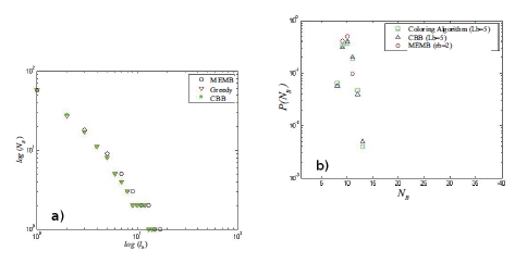
Figure 6.10. a) Comparison of the fractal dimensions obtained by the application of the three algorithms to the IEEE 57-node network (the number of executions of each algorithm is 102). b) Comparison of the distributions of the number of boxes NB necessary to cover the IEEE 57-node network (the number of realizations of each algorithm is 103). For a color version of this figure, see www.iste.co.uk/heliodore/metaheuristics.zip

Figure 6.11. Fractal dimension of the Colombian network (in red, the CBB algorithm and in blue the MEMB algorithm). Case of the Colombian network (1,873 nodes)
In conclusion, it appears that the notion of graph fractal dimension of electrical networks can have a legitimate existence. We will not go further with the interpretation because additional tests must be established to strengthen the physical meaning. In particular, one of the avenues that we are conceiving is to consider the perspective of scale relativity developed by Nottale [NOT 11] in which the notion of fractal dimension becomes relative and consequently is no longer a constant.
6.3.3. Network robustness
In the previous sections, a few indicators of the topology of electric networks have been outlined. Therefore, the determination of the general characteristics of a network, namely the degree distribution, the clustering coefficient, the diameter, etc., have allowed us to gain an overall perspective (in statics) about the robustness of a network by comparing it to already existing models (small-world, “scale-free”, random graphs, etc.). In this section, we are going to look at the robustness of electrical networks by simulating faults therein.
The safety of a network breaks down into two subproblems, static and dynamic:
- – a static robustness study refers to the fact that no consideration of the power flow, and possibly of information flow, are taken into account;
- – a dynamic study of robustness needs to take into consideration power flows circulating in the electric network. In other words, when a fault occurs in a node or a link of the electrical network, a redistribution of power flows is performed in order to determine the state t + 1 of the network.
In the following, we will mainly focus on the static robustness of complex networks.
Several efficiency measures can be used as network robustness indicators [NEW 03, DOR 08, BOC 06]. For instance, it is possible to study a network by quantifying the largest connected component (or subnetwork) after voluntary and random removal of a fraction of the system components, commonly known as fault, or after removing a fraction of components of the utmost importance (more precisely, the nodes with a strong degree, high load, etc.), commonly known as attack. The larger the size of the largest connected component is, the more reliable the network remains. Moreover, the mean of geodesic paths L (equation [6.17]), which can be replaced by E the overall or Eloc the local efficiency (which are the harmonic means of the geodesic paths between each node, equation [6.18]), is another network indicator of the robustness [CRU 05, MOT 02]. A highly robust network has thus an overall efficiency close to 1.
Another approach to measure the network robustness consists very simply of counting the number of defective elements in the system [CAR 09]. Other robustness indicators can be defined depending on the type of network, such as the loss of connectivity CL utilized in [ALB 04]:

where NG is the total number of generators and ![]() is the number of generators connected to the node i.
is the number of generators connected to the node i.
The study of the robustness of a network by means of removing an element of the system is called “N-1 study” (or N-1 contingency) [BOC 06, ROZ 09].
Faults (Figure 6.12(a)) and attacks simulations (Figure 6.12(b)) have been made with our real test network, the Colombian electrical network. Indicators such as the overall efficiency, the mean geodesic path, the diameter and the size of the giant component indicate that the Colombian network is vulnerable to attacks and moderately robust to faults. Indeed, it can be observed that removing a ratio of 10% of the most important nodes (attack case) is enough for the network to break down. However, in the event of faults, a ratio of 50% of the nodes is necessary for the network to collapse.
However, although the network is scale-free, it is, nevertheless, slightly more robust to attacks than a scale-free graph model of the Barabási type. In fact, simply removing 2% of highest degree nodes in the Barabási network is enough for it to sag.
This slight difference can be explained by the fractal character of the Colombian network, which we have developed in section 6.3.2. The latter can increase robustness to intentional attacks if compared to the robustness of scale-free networks having the same exponent γ = 3.26. In effect, the fractal property provides better protection when “hubs” are removed from the system due to dispersion effect (isolation of “hubs” between them).

Figure 6.12. Robustness of the Colombian network: a) to faults and b) attacks
6.4. Conclusion
This chapter is dedicated to the topological study of electrical networks, including the Colombian network. First, a few indicators and observables, which have been helpful in guiding us in the description of electric networks, have been presented and then applied to the Colombian electrical network.
After examination of the different results obtained, four key findings can be outlined concerning the Colombian network:
- – the Colombian network proves to be particularly vulnerable to attacks (intentional faults) and moderately robust to random failures. Therefore, it suffices that 10% of the nodes of stronger degree do break down for the whole network to become inoperative;
- – the Colombian network exhibits “scale-free” properties, which would explain its vulnerability with regard to intentional attacks;
- – nevertheless, the Colombian network, which is also the case of the Northeastern American network, a priori presents fractal properties, which would enable it to be a little more robust to attacks than “scale-free” networks;
- – because of its low consolidation coefficient, the Colombian network is not “locally” efficient, inasmuch as it does not belong to the family of small-word networks.