
5
Genetic Algorithm-based Wind Farm Topology Optimization
5.1. Introduction
A wind farm installation consists of using the wind to rotate a large-sized propeller. When the wind reaches the propeller, the particular shape of the blades allows it to easily be put into motion. At a height, the wind is stronger because it is free from the roughness of the ground. The propeller is therefore placed on top of a tower of several tens of meters. The addition of an automatic system enables the wind turbine to be placed facing the wind, which increases its efficiency. When the propeller starts to turn, it acquires the energy of the motion transmitted by the wind. The latter is then transformed into electric energy due to the dynamo effect and sent into the network.
Several wind turbines can be grouped on the same site to form a wind farm. In this case, maintenance is simpler and billing is easier. On the other hand, the operating strategy and the management of the complexity and risks incurred by such a farm become a sensitive matter. These difficulties include connecting wind turbines to the electric grid, which is not an easy task for operators. As a matter of fact, given the high cost of wires, the cost of feeders and their eventual unavailability, a bad interconnection in a wind farm can result in very significant safety and pecuniary losses.
In this chapter, the main objective of the work carried out was to satisfy a specific requirement, namely the implementation of a computational tool which makes it possible to “optimally” determine the interconnection of a wind farm. This study has been voluntarily achieved over a limited time period in order to validate, on the one hand, the contribution of optimization techniques, especially that of genetic algorithms, and, on the other hand, to develop a computational tool that can be directly exploited by the user.
5.2. Problem statement
Wind energy is one of the main components of renewable energy sources. Apart from the difficulty in designing wind farms (position facing the wind, wind turbine height, etc.), the connection to the electric network turns out to be a difficult task from an expert point of view.
5.2.1. Context
Wind power project developers can resort to tools for decision support during the design of their farm, in particular for the optimization of the internal electrical architecture. Their requirements mainly take into consideration the definition:
- – of the internal network topology of the farm (20 kV or 33 kV);
- – of the cable type of this internal network (section);
- – of the location of the substation (MV/HV) in the case of an offshore wind farm with platform;
- – of the substation configuration (MV/HV);
- – of compensation requirements.
The first three points can be formulated in the form of an optimization problem and solved via a metaheuristic.
In this design phase of the farm, developers have knowledge:
- – of the masts layout map (X, Y coordinates of wind turbines);
- – of the location of the substation (MV/HV) for connection to the electric grid and thus of the connection voltage level (HV);
- – of the turbine type (P, Q, U diagrams);
- – of cables’ parameters (section, impedance, cost, etc.).
The parameters of the cables (section, impedance, cost, etc.) are standardized. As an application of our decision-support tool, the values in Table 5.1 will be used for buried cables. However, this type of table is dedicated to a particular project.
Table 5.1. Reference parameters by phase for buried cables 33 kV (onshore farm)

The option of placing two cables in parallel can be considered, if the power to evacuate requires it. In this case, a declassifying factor is applied to the maximal current-carrying capacity in parallel lines (typically 0.83).
In this chapter, a group of wind turbines radially connected to a substation is called a “cluster”. Figure 5.1 represents a four-clustered topology. The cost of an MV feeder is estimated at e20,000.
It should be noted that the present problem can be modeled in the form of a multiobjective problem. As a matter of fact, increasing the number of clusters:
- – increases the number of feeders (cost deterioration);
- – decreases cable section (cost reduction);
- – increases the availability of the farm (the loss of a feeder is less critical) and makes maintenance easier.
In this case, the number of feeders (clusters) is no longer a decision variable but rather a criterion to be optimized, which will reduce, without any doubt, the number of possibilities for interconnections (Table 5.3). On the other hand, this will complicate the problem’s solution. This is the reason why initially we focused on solving the problem in its single-objective form.
In the case of an offshore farm, it is possible for an MV/HV substation to be installed on a platform. The positioning of this platform is free (provided a safety distance of 100 m from the nearest wind turbine). The offshore platform substation is then connected in HV to the onshore substation of the electrical network (via an HV submarine cable).

Figure 5.1. Four-cluster solution
The criterion to be minimized is a cost criterion consisting of four basic costs, namely:
- – cable cost (depending on their length and their section);
- – Joule losses cost (according to the resistance and current flowing in the cable);
- – feeder cost (depending on the number of clusters);
- – non-distributed energy cost (depending in particular on the number of clusters).
As in the majority of real optimization problems, the objectives to minimize are subject to a set of constraints, which complicates the problem’s solution. In this case, the minimization of the “cost” must take into account the following constraints:
- – it is necessary to ensure that the number of different sections used in cables remains below a certain value (typically no more than five types of sections);
- – the types of cable used must be those in Table 5.1;
- – the crossing of cables is to be avoided;
- – the voltage drop in a cluster must be less than 2%;
- – each wind turbine can have only one or two feeders (see Figure 5.2);
- – all turbines must be connected (directly or via other turbines) to the connection substation;
- – the positioning of masts is not reversible;
- – the current-carrying capacity for each cable must be higher than the current flowing through the cable under consideration.

Figure 5.2. Connection of a wind turbine (1/2 feeders)
5.2.2. Calculation of power flow in wind turbine connection cables
For power flow calculations, we consider the most critical case in terms of losses, permanent maximum current and voltage drop, namely:
- – each turbine is operating at Pmax, Qmax;
- – a minimal voltage at the supply point (MV/HV substation).
Furthermore, it should be noted that cables are modeled by an electrical π model.
5.2.2.1. Calculation of non-distributed energy
The optimization algorithm requires, among other things, a cost criterion (or objective function). The latter is based on the cost of Joule losses in cables and on the cost of the initial investment related to the lengths and types of cable used. It is also important to recall that the voltages calculated at each of the nodes verify imposed constraints (the voltage drop along a cluster must be less than 2%).
Joule losses are determined by the calculation of the current in each cable (through an AC Power Flow based calculation.) This latter also provides the voltage in each node. Losses and resulting voltages will be used for the calculation of the objective function described hereafter.
The goal is to determine the cost of non-distributed energy updated over 20 years. In fact, if a failure occurs in circuit breakers or in transformers, the energy produced by wind turbines cannot be distributed. This represents a loss of profit that must be quantified.
Each feeder is associated with an average downtime μ per year (typically μc = 5 h/year). The average downtime μf of the farm is therefore:
From which, the non-distributed energy cost Σe is expressed as:

In the end, the formula for the cost of non-distributed energy is:

and designated by:
- – Nd, the number of feeders (clusters);
- – Pmax, the maximal power (nominal power) of the wind farm;
- – κ, the load factor (that is the mean power actually produced from the nominal power);
- – τ, the update rate;
- – ψ, the redemption price of the KW/h.
The calculation of non-distributed energy is achieved on the basis of the data in Table 5.2.
Table 5.2. Parameters to be used for the calculation of non-distributed energy
| Redemption price MWh(e) | 180 |
| Factor load | 0.34246575 |
| Update rate | 2 % |
| Cluster downtime (μc in h/year) | 5 |
5.2.2.2. Computation of losses cost
Joule losses are evaluated according to the formula φ = RI2.
The purchase price ψ of the MWh allows the cost of losses to be quantified (Table 5.2). These losses must also be updated over 20 years; which amounts to stating that losses costs Σp are calculated as follows (equation [5.4]):
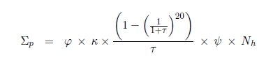
At this level of formalism, all the ingredients necessary to understanding, to the calculations of installation costs and to the modeling of the interconnection problem of a wind farm are drafted. In summary, the decision-support tool, which will be detailed in the following sections assumes as parameters and input variables:
- – the layout of the masts plan in the form of (X, Y) coordinates;
- – the location of the onshore substation in the form of (X, Y) coordinates;
- – the wind turbine type (Pmax, Qmax);
- – the parameters of cables to use (section, R, L, C, ampacity I, cost, Unominal);
- – the feeder cost;
- – the MWh purchase price;
- – the projected load factor of the farm;
- – the cluster downtime;
- – the update rate.
On output, the optimization program that will be implemented return, as output variables:
- – the internal network topology of the farm;
- – the cable types of this internal network (sections);
minimizing losses Σ in the internal network of the farm (equation [5.5]):
where Σe and Σp, respectively, are the non-distributed energy cost and the losses cost, defined earlier.
Although the problem that is described in this section is purely combinatorial and non-hybrid, it, nevertheless, presents a complexity which increases very quickly with the number of wind turbines to be connected. As a matter of fact, the number of possibilities (for configurations) is of the order of:
where n denotes the number of existing turbines in the farm and Nb_Type refers to the number of cable types available, namely (n − 1) × (Nb_Type)n times more complex than the traveling salesman problem.
Table 5.3 shows the combinatorial explosion of the problem. It is assumed that one configuration is evaluated in 1 μs.
Table 5.3. Number of possibilities for five cable types based on the number of wind turbines
| Number of wind turbines | Number of possibilities | Computational time |
|---|---|---|
| 5 | 1,500,000 | 1.5 sec |
| 10 | 3.1894e+014 | 10 years |
| 15 | 5.5870e+023 | 17,716 billion years |
| 20 | 4.4084e+033 | 1.3979e+020 billion years |
| 30 | 7.1640e+054 | 2.2717e+041 billion years |
5.3. Genetic algorithms and adaptation to our problem
5.3.1. Solution encoding
Coding individuals is a crucial phase in the design of a genetic algorithm. It must comprehensively cover the search space and satisfy, among other things, the maximum number of constraints. Crossover and mutation operators should be easily adaptable to the chosen type of encoding.
Within the context of our problem, an individual (chromosome) is represented as follows:
where ![]() form a permutation, li ∈ {1, −i}:
form a permutation, li ∈ {1, −i}:
- – when li is equal to 1, this means that the element Ei+1 of the permutation is connected to the connection substation;
- – when li is equal to −i, this means that the element Ei+1 of the permutation is connected to the element Ei of the same permutation.
Such coding ensures that all turbines be connected and that each turbine be connected at most to only two elements (turbine or connection substation).

Figure 5.3. Graph corresponding to the individual Example_Coding. For a color version of this figure, see www.iste.co.uk/heliodore/metaheuristics.zip
EXAMPLE 5.1.– The graph corresponding to the next Example_Coding individual is shown in Figure 5.3:

In this example, the permutation elements Ei, i ∈ {1, …, 6}, respectively, correspond to wind turbines 2, 4, 1, 5, 3 and 6 and the elements lj, j ∈ {1, …, 6} are, respectively, equal to 1, −1, 1, −3, −4 and 1. The elements l1, l3 and l6 are equal to 1, which means that turbines 2, 1 and 6 are connected to the connection substation. Moreover, the element l4 is equal to −3, which means that the element E4 of the permutation, that is turbine 5, will be connected to the element E3 of the permutation, that is turbine 1 (Figure 5.3).
It should be observed that the element E1 in equation [5.6] is always equal to 1, which means that the turbine corresponding to the first element E1 of the permutation is by default connected to the link substation. Furthermore, a topology that respects the constraints predefined in section 5.2.1 must have at least one turbine connected to the station.
5.3.2. Selection operator
Although this phase does not present any adjustment problems to any selection operator, it is part of the crucial phases of genetic algorithms. In fact, a bad selection of individuals systematically leads to the premature convergence of the algorithm or, if this is the case, to the divergence of the algorithm.
As a general rule, parents are selected for the reproduction phase (crossover) according to their performance (equation [5.7]), where f(Ai) and P[Ai] are, respectively, the performance and the probability with which chromosome Ai will be reintroduced in the new population:
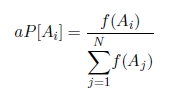
In our case, the selection operator implemented is that of the biased roulette wheel. For this purpose, the procedure is as follows:
- – the individuals of the population are sorted according to performance order by means of equation [5.7];
- – a surface section is attributed to each individual starting from the best to the worst;
- – a random number between [0, 1] is generated;
- – a search is carried out to find out which interval the number generated belongs to and the corresponding individual is selected.
For instance, on four individuals, if the sum of performances equals 10 and if the performance of each individual is, respectively, 2.5, 2, 1 and 4.5, the state of the corresponding biased roulette wheel will be represented as shown in Figure 5.4.
The individual corresponding to the surface (a) has a 45% chance of being selected, whereas the individual corresponding to the white surface has only a 10% chance of being selected.

Figure 5.4. Biased roulette wheel example
To guarantee the elitism of our algorithm, the best individual will be kept at each generation. Furthermore, to avoid a premature convergence of the algorithm, a few bad individuals will be systematically kept (typically two).
5.3.3. Crossover
The crossover operator used in section 5.4 is the one described in [POO 95]. Its principle is the following:
- – given two parents
 and
and 
- – randomly select two crossover positions. Let Pos1 and Pos2 denote these positions;
- – copy the portion
 of the parent P1 into the portion
  of the parent P2;
 - – remove the elements
 .
.
The operator is then defined in two stages and one proceeds as follows.
Stage 1 (search for cycles):
- – given two parents P1 and P2;
- – consider the positions of the elements corresponding to the permutations of the two parents as being unmarked;
- – let i = 1 :
- a) randomly generate an unmarked position (Posi denotes this position and Elti the corresponding element in the permutation of individual P1). Mark the position Posi with i;
- b) let y be the permutation element of the parent P2 corresponding to position Posi:
- – if y = Elti, let i = i + 1 and move to 1 (if there are unmarked positions remaining);
- – otherwise let Posi be the position corresponding to the element y of the permutation of the parent P1 and mark the position Posi with i and move to 2;
- c) at the end of the previous steps, a sequence of numbers is obtained indicating which cycle each element of the two permutations of P1 and P2 belongs to. Denote by Cycle this sequence of numbers.
Stage 2 (mix obtained cycles):
- – randomly create a crossover mask M whose corresponding elements indicate which parent the child will inherit from in each cycle. There are as many elements in the mask as detected cycles (example: if there are three detected cycles, the mask will be, for instance, M = P1P2P1);
- – convert the sequence of numbers Cycle into a permutation based on the mask in the following manner: Cycle(i) ← M(i). For example, if the element i of the digit sequence Cycle equals 2 and M = P1P2P1, then Cycle(i) ← P2. This means that the element 2 of the permutation of the resulting child will inherit element 2 of the permutation of the parent P2.
EXAMPLE 5.2.– The application of the geometric crossover to these two parents is performed in the following manner (Figure 5.5).
Given the two parents in Figure 5.5(a). Let i = 1 and generate a position between 1 and 6 (6 being the number of genes or elements in our coding), let Pos1 = 5 be this position. The cycle i = 1 is then assigned to this position. The value of the element Elt1 corresponding to the parent A equals 1 and that corresponding to the parent B equals 3. A search is performed for the gene that takes 3 as value in the parent A, this gene has position 4. The cycle i = 1 is then assigned to position 4. The element corresponding to position 4 of parent B is equal to 1, which also corresponds to the initial element Elt1, a cycle is then obtained (Figure 5.5(b)). Let i = 2, in other words, a second cycle is searched for, and the same procedure is repeated until all cycles are obtained (all positions are marked).

Figure 5.5. Principle of geometric crossover applied to the two parents A and B. For a color version of this figure, see www.iste.co.uk/heliodore/metaheuristics.zip
Now suppose that all cycles have been identified (Figure 5.5(e)). The sequence of identified cycles is then equal to, in order, {3, 3, 2, 1, 1, 4}. The number of cycles obtained is equal to 4, a four-value mask is then generated in {A, B}, namely ABBA, the mask thus generated. This means that the first cycle is attributed to the parent A, the second and third to the parent B and finally the fourth to parent A. To convert the sequence {3, 3, 2, 1, 1, 4} in a permutation, the values 1, 2, 3 and 4 therefore have to be replaced by A, B, B and A, respectively, which yields: {3, 3, 2, 1, 1, 4} ⇒ {B, B, B, A, A, A}.
Figure 5.6(c) represents the graph of the child obtained by crossing over the parents A and B in Figure 5.5. This figure shows that the resulting child has indeed inherited from both parents. In effect, wind turbines 1 and 4 of the child are only connected to the link substation, which is the signature of the parent A. Moreover, the connection of turbines 6, 5 and 3 has the same signature as parent B.

Figure 5.6. Graphical representation of the example of the crossover in Figure 5.5: a) parent A, b) parent B, and c) the child obtained by crossing over parent A and B. For a color version of this figure, see www.iste.co.uk/heliodore/metaheuristics.zip
REMARK 5.1.– In our application cases, the geometric crossover is applied to the permutations of individuals with high probability, whereas conventional crossover described in section 2.2 is applied to the second part (the links li)of individuals with low probability.
5.3.4. Mutation
Unlike crossover, standard mutation operators can, usually, be adapted to any type of coding. In our coding case, the mutation of individuals is achieved as follows:
- – generate a position Pos1 where the mutation can take place;
- – if position Pos1 corresponds to the “permutation” portion of the individual then (Figure 5.7(a)):
- - generate another position Pos2, corresponding to the “permutation” part of the individual;
- - permute the two elements corresponding to both positions Pos1 and Pos2;
- – otherwise, with fair probabilities:
- - increase, if possible, the number of turbines connected to the substation by 1, that is;
- - generate a position in the second part of the individual whose elements are negative;
- - mutate the corresponding element in 1 (Figure 5.7(b));
- - decrease, if possible, by 1 the number of wind turbines, connected to the substation, that is;
- - generate a position in the second part of the individual whose elements are equal to 1, namely position Posi;
- - mutate the corresponding element in −i (Figure 5.7(c));
- - randomly change the position of one of the elements equal to 1 of the second portion of the individual (do not alter the first 1 because the first element of the permutation is always connected to the stepup substation) (Figure 5.7(d)).

Figure 5.7. Mutation examples of an individual. For a color version of this figure, see www.iste.co.uk/heliodore/metaheuristics.zip
Therefore, the mutation operator defined as such allows any topology to be obtained, namely, the modification the turbines order within a cluster (Figure 5.8(b)), the addition of a cluster (Figure 5.8(c)), the removal of a cluster (Figure 5.8(d)) and finally, modification the number of turbines in each cluster (Figure 5.8(e)).
In addition, managing constraints in section 5.2.1 becomes simpler:
- – the encoding thus defined in section 5.3.1 takes into account constraints 5 and 6, discussed in section 5.2.1;
- – constraint 2 is an input variable; it is therefore considered a priori and cannot be breached, similarly for constraint 7;
- – constraint 4 is taken into consideration by penalizing the objective function in the event of a breach;
- – placing two cables in parallel, eventually several cables, makes it possible to satisfy constraint 8 in the event of overloading (that is to say, current too high);
- – constraint 3 is not explicitly taken into account in the optimization process. However, due the high cost of cables, an optimal solution will necessarily involve few crossings, or even none (in a quadrilateral, the sum of the two diagonals is greater than the sum of both sides). In addition, the solutions which comprise cables that are too long will be penalized, which will favor the connection of turbines with their closest neighbors.
5.4. Application
Although on average a farm only comprises around 20 turbines, it is nonetheless considered as part of the world of electric networks. Consequently, similarly to all electric networks, it is governed by the equations and the constraints of the Power Flow model described in section 4.3.1. Thus, power flows circulating in a given topology are only valid if they satisfy equations in section 4.3.1. The nonlinear system of this model can easily be solved by descent methods and, in particular, Newton–Raphson-based methods.

Figure 5.8. Mutation examples: a) the graph in Figure 5.7, b) modification of the turbines order in a cluster, c) addition of a cluster, d) removal of a cluster and e) modification of the number of turbines in a cluster. For a color version of this figure, see www.iste.co.uk/heliodore/metaheuristics.zip
The calculation of the current in each cable and of the voltage in each node is carried out by a function (NewtonPF) from the Pylon module, which is a translation in Python 2.6 of the Matlab Matpower program for Power Flow computations.
This function assumes the description (topology) of the network of cables interconnecting the turbines as input, that is:
- – the definition of buses (bus type, active and reactive power demand, etc.);
- – the definition of branches between buses (numbers of buses connected to each branch, resistance p.u., reactance p.u., susceptance p.u., etc.);
- – the definition of generators (number of buses to which the generators are connected, active and reactive powers generated, etc.).
The NewtonPF function provides, as output, the voltage p.u. in each node (amplitude and phase) and the admittance matrix.
The currents p.u. in branches (amplitude and phase) are calculated by means of the admittance matrix determined by NewtonPF. A test is also carried out to know if currents in branches are compatible with the current-carrying capacity of the cable type of each branch. If necessary, and taking into account a declassification factor, the number of cables in parallel is corrected such as to comply with this constraint. In this case, if the number of cables in parallel has been changed in at least one branch, the Power Flow computation is relaunched.
Throughout applications that follow, the parameters of the algorithm will be fixed as follows:
- – number of iterations: 1,000 (arbitrarily fixed, for a reasonable computation time);
- – population size: 50;
- – mutation probability: Pm =0.1;
- – crossover probability: Pc =0.8;
- – Pmax : 1 MW;
- – Qmax : 0.283 MW;
- – number of regenerated individuals: 20% of the initial population;
- – cable types: those in Table 5.1 of section 5.2.1;
- – redemption price, load factor, update rate and downtime of a cluster: those in Table 5.2 of section 5.2.1;
- – feeder cost; €20,000.
5.4.1. Application to farms of 15–20 wind turbines
Figure 5.9 shows the wiring proposed by the algorithm of a farm comprising 15 turbines. The outputs summary is presented in Table 5.4.

Figure 5.9. Topology of a farm with 15 turbines obtained by the genetic algorithm. For a color version of this figure, see www.iste.co.uk/heliodore/metaheuristics.zip
Figure 5.10 shows the wiring proposed by the algorithm of a farm comprising 20 turbines. The outputs summary is presented in Table 5.5.
5.4.2. Application to a farm of 30 wind turbines
Figure 5.11 shows the wiring proposed for a farm comprising 30 turbines. The outputs summary is presented in Table 5.6. The figure on the top-left represents the evolution of the three economic criteria (non-distributed energy cost, cables cost and joule losses cost) defined in section 5.2.1. The figure center-left represents the evolution of the objective function of the problem being addressed (the sum of the three economic costs defined in section 5.2.1). The bottom-left figure represents voltage drops at the edges of the turbines (as a percentage of the nominal voltage). Finally, the large figure to the right represents the topology of the wind farm proposed by the genetic algorithm.
Table 5.4. Outputs summary of a solution corresponding to a farm of fifteen turbines
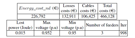

Figure 5.10. Topology of a farm with 20 turbines obtained by the genetic algorithm. For a color version of this figure, see www.iste.co.uk/heliodore/metaheuristics.zip
Table 5.7 represents the detail of the solution outputs corresponding to Figure 5.11.
Table 5.5. Outputs summary of a proposed solution corresponding to a farm of twenty turbines

Table 5.6. Outputs summary of a solution proposed by genetic algorithm, corresponding to a farm of thirty turbines


Figure 5.11. Topology of a farm with 30 turbines obtained by the genetic algorithm. For a color version of this figure, see www.iste.co.uk/heliodore/metaheuristics.zip
Table 5.7. Outputs details of a solution proposed by genetic algorithm, corresponding to a farm of thirty wind turbines

5.4.3. Solution of a farm of 30 turbines proposed by human expertise
Figure 5.12 shows the wiring proposed by human expertise for the same farm comprising 30 wind turbines. The summary of the outputs is presented in Table 5.8.

Figure 5.12. Topology of a farm of 30 turbines proposed by human expertise. For a color version of this figure, see www.iste.co.uk/heliodore/metaheuristics.zip
It should be observed from Tables 5.7 and 5.8 that the genetic algorithm reduces the costs by 22.5% compared to the solution proposed by human expertise.
Table 5.9 presents the details of outputs from the solution corresponding to Figure 5.12, which can then be compared to Table 5.7.
Table 5.8. Outputs summary of a solution proposed by human expertise, corresponding to a farm of thirty turbines

5.4.4. Validation
The solutions obtained, on the one hand, by an expert and, on the other, numerically by means of a “genetic algorithm” are absolutely consistent. It has been found that the numerical solution exhibits an advantage that makes it possible to reduce costs by about 22%: this result is therefore significant.
The choice on genetic algorithms was conditioned by the discrete nature of the problem. Nevertheless, it seems natural to substitute them with population-based techniques (particle swarms, ant colonies, etc.).
5.5. Conclusion
In this chapter, a tool for decision making using genetic algorithms has been proposed. This tool can be utilized by electric network operators aiming to optimize the internal topology of their wind farms. Initially, an encoding model efficient for this kind of problem was proposed. We have seen through supported examples that this type of encoding gives significant flexibility regarding constraint management and the implementation of our genetic algorithm. Second, the implementation of a Python function performing an AC Power Flow computation was carried out. It is based only on Python code whose sources are accessible and free (Pylon module). We are therefore totally free from the MATLAB/MATPOWER environment whose usage implies costs that can be quite high. Although this is not mentioned in this chapter, a validation of this code by comparing the results given by a similar MATLAB/MATPOWER program has been successfully conducted.
Thus, entirely developed based on the Python platform, the executable available (version 1.0) allows for the determination of relevant solutions concerning the internal connection of a wind farm. A second version will enable the time necessary for the computation to obtain an “optimal” solution to be reduced.
Table 5.9. Outputs details of a solution proposed by human expertise, corresponding to a farm of thirty wind turbines

The following elements are to be considered:
- – based on the choices made, the number of iterations and the size of the population can be parametrized;
- – the initialization of the genetic algorithm makes it possible to decrease the exploration domain in a meaningful way. The introduction of physical considerations should enable an acceleration of convergence;
- – the graphical interface developed does not constitute a final version. It can be re-laid out at will, depending on the user’s desiderata.
The design of the genetic algorithm (selection, crossover and mutation) may be the subject of further reflection. A preliminary study will then be required in order to identify sustainable avenues concerning the optimality of the solution.