9

Reversing Bytecode Languages – .NET, Java, and More

The beauty of cross-platform compiled programs is in their flexibility as you don’t need to spend lots of effort porting each program to different systems. In this chapter, we will learn how malware authors are trying to leverage these advantages for malicious purposes. In addition, you will be provided with an arsenal of techniques and tools whose aim is to make analysis quick and efficient.

In this chapter, we will cover the following topics:

• The basic theory of bytecode languages
• .NET explained
• .NET malware analysis
• The essentials of Visual Basic
• Dissecting Visual Basic samples
• The internals of Java samples
• Analyzing compiled Python threats

The basic theory of bytecode languages

.NET, Java, Python, and many other languages are designed to be cross-platform. The corresponding source code doesn’t get compiled into an assembly language (such as Intel, ARM, and so on), but gets compiled into an intermediate language that is called bytecode language. Bytecode language is a type of language that’s close to assembly languages, but it can easily be executed by an interpreter or compiled on the fly into a native language (this depends on the CPU and operating system it is getting executed in) in what’s called Just-in-Time (JIT) compiling.

Object-oriented programming

Most of these bytecode languages follow state-of-the-art technologies in the programming and development fields. They implement what’s called object-oriented programming (OOP). If you’ve never heard of it, OOP is based on the concept of objects. These objects contain properties (sometimes called fields or attributes) and contain procedures (sometimes called functions or methods). These objects can interact with each other.

Objects can be different instances of the same design or blueprint, which is known as a class. The following diagram shows a class for a car and different instances or objects of that class:

Figure 9.1 – A car class and three different objects

In this class, there are attributes such as fuel and speed, as well as methods such as accelerate() and stop(). Some objects could interact with each other and call these methods or directly modify the attributes.

Inheritance

Another important concept to understand is inheritance. Inheritance allows a subclass to inherit (or include) all the attributes and methods that are included in the parent class (with the code inside). This subclass can have more attributes or methods, and it can even reimplement a method included in the parent class (sometimes called a super or superclass).

Polymorphism

Inheritance allows one class to represent many different types of objects in what’s called polymorphism. A Shape class can represent different subclasses, such as Line, Circle, Square, and others. A drawing application can loop through all Shape objects (regardless of their subclasses) and execute a paint() method to paint them on the screen or the program canvas without having to deal with each class separately.

Since the Shape class has the paint() method and each of its subclasses has an implementation of it, it becomes much easier for the application to just execute the paint() method, regardless of its implementation.

.NET explained

.NET languages (mainly C# and VB.NET) are languages that were designed by Microsoft to be cross-platform. The corresponding source code is compiled into a bytecode language, originally named Microsoft Intermediate Language (MSIL), which is now known as Common Intermediate Language (CIL). This language gets executed by the Common Language Runtime (CLR), which is an application virtual machine that provides memory management and exception handling.

.NET file structure

The .NET file structure is based on the PE structure that we described in Chapter 3, Basic Static and Dynamic Analysis for x86/x64. The .NET structure starts with a PE header that contains the last but one entry in the data directory pointing to .NET’s special CLR header (COR20 header).

.NET COR20 header

The COR20 header starts after 8 bytes of the .text section and contains basic information about the .NET file, as shown in the following screenshot:

Figure 9.2 – CLR header (COR20 header) and CLR streams

Some of the values of this structure are as follows:

• cb: Represents the size of the header (always 0x48)
• MajorRuntimeVersion and MinorRuntimeVersion: Always with values of 2 and 5 (even with runtime 4)
• Metadata address and size: This contains all the CLR streams, which will be described later
• EntryPointToken (or EntryPointRVA): This represents the entry point – for example, for the 0x6000012 value, we have the following:
  • 0x06: Represents the sixth table of the #~ stream (we will talk about streams in detail later). In the following screenshot, we can see that it corresponds to the Methods table.
  • 0x0012 (18): Represents the method ID in the aforementioned table (in this case, number 6). As shown in the following screenshot, the pointed method here is Main:

Figure 9.3 – The entry point method in the methods table in the first stream, #~

Now, let’s talk about streams.

Metadata streams

Metadata contains five sections that are similar to the PE file sections, but they are called streams. The streams’ names start with # and are as follows:

• #~: This stream contains all the tables that store information about classes, namespaces (classes' containers), events, methods, attributes, and so on. Each table has a unique ID (for example, the Methods table has an ID of 0x6).
• #Strings: This stream includes all the strings that are used in the #~ stream. This includes the methods’ names, classes’ names, and so on. Here, each item starts with its length, followed by the string, and then the next item’s length followed by the string, and so on.
• #US: This stream is similar to the #Strings stream, but it contains the strings that are used by the application itself, as shown in the following screenshot (with the same structure of item length followed by the string):

Figure 9.4 – The #US Unicode string started with the length and was followed by the actual string

• #GUID: Stores the unique identifiers (GUIDs).
• #blob: This stream is similar to #US and #Strings, but it contains all Binary data related to the application. It has the same format as the item length, followed by the data blob.

So, this is the structure of the .NET application. Now, let’s look at how to distinguish the .NET application from other executable files.

How to identify a .NET application from PE characteristics

The first way that a .NET PE file can be identified is by using a PEiD or CFF Explorer that includes signatures that cover .NET applications, as shown in the following screenshot:

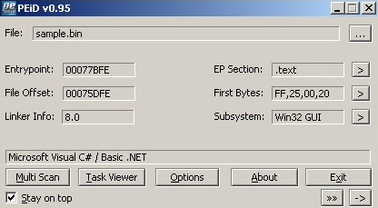
Figure 9.5 – PEiD detecting that malware is a .NET application

The second way is to check the import table inside the data directory. .NET applications always import only one API, which is _CorExeMain from mscoree.dll, as shown here:

Figure 9.6 – .NET application import table

Finally, you can check the last but one (15th) entry in the data directory, which represents the CLR header. If it’s populated (that is, contains values other than NULL), then it’s a .NET application, and this should be a CLR header (you can use CFF Explorer to check that).

The CIL language instruction set

The CIL (also known as MSIL) language is quite similar to Reduced Instruction Set Computer (RISC) assembly languages. However, it doesn’t include any registers, and all the variables, classes, fields, methods, and so on are accessed through their ID in the streams and their tables. Local variables are also accessed through their ID in methods. Most of the code is based on loading variables and constants into the stack, performing an operation (whose result is stored on the stack), and popping this result back into a local variable or field in an object.

This language consists of a set of opcodes and arguments for these opcodes (if necessary). Most of the opcodes take up 1 byte. Let’s take a look at the instructions in this language.

Pushing into stack instructions

There are many instructions for storing values or IDs in the stack. These can be accessed later by an operation or stored in another variable. Here are some examples of them:

Important Note

For all the instructions that take an ID, they take an ID in a 2-byte form. There is a shorter version of them that has the .s suffix added to them, which takes an ID in a 1-byte form.

The instructions that deal with the constants or elements of an array (ldc and ldelem) take a suffix that describes the type of that value. Here are the used types:

Now, let’s learn how to pull a value from the stack out into another variable or field.

Pulling out a value from the stack

Here are the instructions that let you pull out (pop) a value or a reference from the stack into another variable or field:

Important Note

The instructions that take IDs also have a shorter version with the .s suffix. Some instructions, such as stind and stelem, may have a value type suffix as well (such as .i4 or .r8).

Mathematical and logical operations

The CIL language implements the same operations that you will see in any assembly language, such as add, sub, shl, shr, xor, or, and, mul, div, not, neg, rem (the remainder from a division), and nop (for no operation).

These instructions take their arguments from the stack and save the result back into the stack. These can be stored in a variable using any store instruction (such as stloc).

Branching instructions

This is the last important set of instructions to learn. These instructions are related to branching and conditional jumps. These instructions are not so different from the assembly languages either, but they depend on the stack values for comparing and branching:

Now, let’s put this knowledge into practice and learn how the source code would translate into these instructions.

CIL language into higher-level languages

So far, we’ve discussed the various IL language instructions and the key differentiating factors of a .NET application, as well as its file structure. In this section, we will take a look at how these higher-level languages (VB.NET, C#, and others), as well as their statements, branches, and loops, get converted into CIL language.

Local variable assignments

Here is an example of setting a local variable value with a constant value of 10:

X = 10;

This will be converted into the following:

ldc.i4 10  // pushes an int32 constant with value 10 to the stack

stloc.0  // pops a value to local variable 0 (X) from stack

Easy peasy.

Local variable assignment with a method return value

Here is another more complicated example that shows you how to call a method, push its arguments to the stack, and store the return value in a local variable (here, it’s calling a static method from a class directly and not a virtual method from an object):

Process[] Process = System.Diagnostics.Process::GetProcessesByName("App01");

The intermediate code looks like this:

ldstr "App01" // here, ldstr accesses that string by its ID and the string itself is located in the #US stream

call class [System]System.Diagnostics.Process[] [System]System.Diagnostics.Process::GetProcessesByName(string)

Stloc.0       // store the return value in local variable 0 (X)

Basic branching statements

For if statements, the C# code looks like this:

if (X == 50)
{
  Y = 20;
}

The corresponding IL code will look like this (here, we are adding the line numbers for branching instructions):

00: ldloc.0  // load local variable 0 (X)

01: ldc.i4.s 50  // load int32 constant with value 50 into the stack

02: bne 5       // if not equal, branch/jump to line number 5

03: ldc.i4.s 20 // load int32 constant with value 20 into the stack

04: stloc.1     // place the value 20 from the stack to the local variable 1 (Y)

05: nop       // here, it could be any code that goes after the If statement

06: nop

These instructions will also help us understand the next topic – loops.

Loops statements

The last example we will cover in this section is the for loop. This statement is more complicated than if statements and even more complicated than the while statement for loops. However, it’s more widely used in C#, and understanding it will help you understand other complicated statements in the IL language. The C# code looks like this:

for (i = 0; i < 50; i++)
{
  X = i + 20;
}

The equivalent IL code will look like this:

00: ldc.i4.0 // pushes a constant with value 0

01: stloc.0  // stores it in local variable 0 (i). This represents i = 0

02: br 11    // unconditional branching to line 11

03: ldloc.0  // loads variable 0 (i) into stack

04: ldc.i4.s 20 // loads an int32 constant with value 20 into stack

05: add      // adds both values from the stack and pushes the result back to stack (i + 20)

06: stloc.1  // stores the result in a local variable 1 (X)

07: ldloc.0  // loads local variable 0 (i)

08: ldc.i4.1 // pushes a constant value of 1

09: add      // adds both values

10: stloc.0  // stores the result in local variable i (i++)

11: ldloc.0  // loads again local variable i (this is the branching destination)

12: ldc.i4.s 50 // loads an int32 constant with value 50 into stack

13: blt.s 3  // compares both values from stack (i and 50) and branches to line number 3 if the first value is lower

That’s it for the .NET file structure and IL language. Now, let’s learn how to analyze .NET malware.

.NET malware analysis

As you may know, .NET applications are easy to disassemble and decompile so that they become as close to the original source code as possible. This leaves malware more exposed to reverse engineering. We will describe multiple obfuscation techniques in this section, together with the deobfuscation process. First, let’s explore the available tools for .NET reverse engineering.

.NET analysis tools

Here are the most well-known tools for decompiling and analysis:

• ILSpy: This is a good decompiler for static analysis, but it can’t debug malware.
• dnSpy: Based on ILSpy and dnlib, it’s a disassembler and decompiler that also allows you to debug and patch code.
• .NET reflector: A commercial decompiler tool for static analysis and debugging in Visual Studio.
• .NET IL Editor (DILE): Another powerful tool that allows you to disassemble and debug .NET applications.
• dotPeek: A tool that’s used to decompile malware into C# code. It’s good for static analysis and for recompiling and debugging with the help of Visual Studio.
• Visual Studio: Visual Studio is the main IDE for .NET languages. It allows you to compile the source code and debug .NET applications.
• SOSEX: A plugin for WinDbg that simplifies .NET debugging.

Here are the most well-known deobfuscation tools:

• de4dot: Based on dnlib as well, it is very useful for deobfuscating samples that have been obfuscated by known obfuscation tools
• NoFuserEx: A deobfuscator for the ConfuserEx obfuscator
• Detect It Easy (DiE): A good tool for detecting.NET obfuscators

In the following examples, we are going to mainly use the dnSpy tool.

Static and dynamic analysis

Now, we will learn how to perform static analysis and dynamic analysis, and then patch the sample to delete or modify the obfuscator code.

.NET static analysis

Multiple tools can help you disassemble and decompile a sample, and even convert it completely into C# or VB.NET source code. For example, you can use dnSpy to decompile a sample by just dragging and dropping it into the application interface. This is what this application looks like:

Figure 9.7 – Static analysis of a malicious sample with dnSpy

You can click on File | Export To Project to export the decompiled source code into a Visual Studio project. Now, you can read the source code, modify it, write comments on it, or modify the names of the functions for better analysis. dnSpy can show the actual IL language of the sample if you right-click and choose Edit IL Language from the menu.

To go to the main function, you can right-click on the program (from the sidebar) and choose Go To Entry Point. However, the main functionality may be located in other functions, such as OnRun, OnStartup, or OnCreateMainForm, as well as in forms. When analyzing code associated with forms, start from their constructor (.ctor) and pay attention to what function is being added to base.Load, as well as what functions are called after this. Some methods, such as the form’s OnLoad method, may be overridden as well.

Another tool that you could use is dotPeek. It’s a free tool that can also decompile a sample and export it to C# source code. It has a very similar interface to Visual Studio. You can also analyze the CIL language using IDA.

Finally, a standard ildasm.exe tool can disassemble and export the IL code of a sample:

ildasm.exe <malware_sample> /output output.il

.NET dynamic analysis

For debugging, there are fewer tools to use. dnSpy is a complete solution when it comes to static and dynamic analysis. It allows you to set breakpoints and step into and step over for debugging. It also shows the variables’ values.

To start debugging, you need to set a breakpoint on the entry point of the sample. Another option is to export the source code to C#, and then recompile and debug the program in Visual Studio, which will give you full control over the execution. Visual Studio also shows the variables’ values and has lots of features to facilitate debugging.

If the sample is too obfuscated to debug or export to C# code by dotPeek or Dnspy, you can rely on ildasm.exe to export the sample code in IL language and use ilasm.exe to compile it again with debug information. Here is how to recompile it with ilasm.exe:

ilasm.exe /debug output.il /output=<new sample exe file>

With the /debug argument, a .pdb file for the sample has been created, which includes its debug information.

Patching a .NET sample

There are multiple ways to modify the sample code for deobfuscating, simplifying the code, or forcing the execution to go through a specific path. The first option is to use the dnSpy patching capability. In dnSpy, you can edit any method or class by right-clicking, selecting Edit Method (C#), modifying the code, and recompiling. You can also export the whole project, modify the source code, go to Edit Method (C#), and click on the C# icon to import a source code file to be compiled by replacing the original code of that class. You can also modify the malware source code (after exporting) in Visual Studio and recompile it for debugging.

In dnSpy, you can modify the local variables’ names by selecting Edit IL Instruction from the menu and selecting Locals to modify them by their local variable names, as shown in the following screenshot. Concerning the classes and methods, you can modify their names just by updating them using the Edit Method (C#) or Edit Class (C#) options:

Figure 9.8 – Editing local variables in dnSpy

You can also edit the IL code directly by selecting Edit IL Instruction and modifying the instructions. This allows you to choose the instruction and the field or variable you want to access.

Dealing with obfuscation

In this section, we will look at different common obfuscation techniques for .NET samples and learn how to deobfuscate them.

Obfuscated names for classes, methods, and others

One of the most common obfuscation techniques is to obfuscate the names of the classes, methods, variables, fields, and so on – basically everything that has a name.

Obfuscation can get even harder if you obfuscate the names into other alphabets or other symbols (since the names are in Unicode), such as Chinese or Japanese.

You can try to deobfuscate such samples automatically by running the de4dot deobfuscator from the command line, like so:

de4dot.exe <sample>

This will rename all the obfuscated names, as shown in the following screenshot (the HammerDuke sample is shown here):

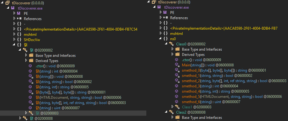
Figure 9.9 – The Hammerduke malware before and after running de4dot to deobfuscate the names

You can also rename the methods manually to add more meaningful names by right-clicking on the method and then selecting Edit Method or clicking Alt + Enter and changing the name of the method. After that, you need to save the module and reload it for the changes to be put into effect.

You can also edit local variable names by right-clicking on the method and choosing Edit Method Body or Edit IL Instructions and choosing Locals.

Encrypted strings inside the Binary

Another common technique used by .NET malware is encrypting its strings. This approach hides these strings from signature-based tools, as well as from less experienced malware analysts. Working with encrypted strings requires finding the decryption function and setting a breakpoint on each of its calls, as shown in the following screenshot:

Figure 9.10 – The Samsam ransomware encrypted strings getting decrypted in memory

Sometimes, there are hard-to-reach encrypted strings, so you may not see them decrypted in the default execution of the malware – for example, because the C&C is down, or maybe there are additional C&C addresses that won’t get decrypted if the first C&C is working. In these cases, you can do any of the following:

• You can try to use de4dot to decrypt the encrypted strings by giving it the method ID. You can find the method ID by checking the Methods table in the #~ stream, as shown in the following screenshot:

Figure 9.11 – The Samsam ransomware myff11() decryption function, ID 0x0600000C

Then, you can decrypt the strings dynamically using the following command:

de4dot <sample> --strtyp delegate --strtok <decryption method ID>

• You can modify the entry point code and add a call to the decryption function to decrypt the strings. The preceding screenshot is created by repointing calls to the decryption functions, including the encrypted strings. For dnSpy to process this code, you must use these strings by changing an object field or calling System.Console.Writeline() to print that string to the console. You will need to save the module after modifying it and reopen it for the changes to be put into effect.

Another option is to export the whole malware source code from dnSpy by clicking on File | Export To Project (other tools may have similar functionality), modifying it, and then recompiling it with Visual Studio before debugging it.

The sample is obfuscated using an obfuscator

There are many .NET obfuscators publicly available. They are generally supposed to be used for protecting intellectual property, but they are also commonly used by malware authors to protect their samples from reverse engineering. There are multiple tools for detecting known packers, such as Detect It Easy (DiE), as shown in the following screenshot:

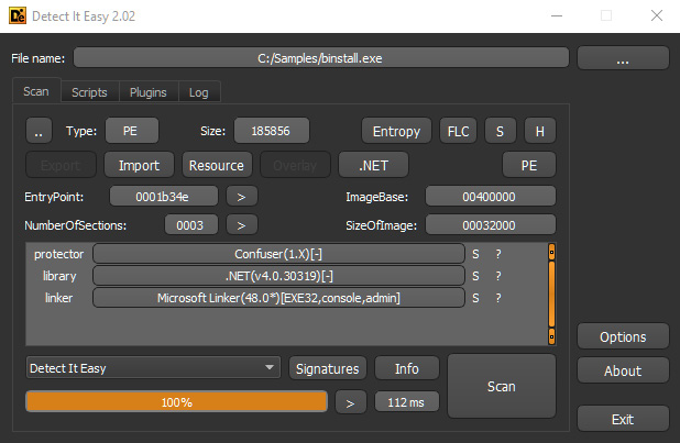
Figure 9.12 – Detect it Easy detecting the obfuscator (ConfuserEx) used to protect against malware

You can also use the de4dot tool to detect the obfuscator by only running the de4dot.exe -d <sample> command or deobfuscate the sample using the de4dot.exe <sample> command.

For custom and unknown obfuscators, you will need to go through debugging and patching processes to deal with them. Before doing so, check different sources, if there are solutions or deobfuscators for it. If the obfuscator is shareware, you may be able to communicate with the authors and get their aid to deobfuscate the sample (as these obfuscators are not designed to help malware authors protect their samples).

Compile after delivery and proxy code execution

Instead of distributing malicious .NET binaries directly, attackers may also attempt to dynamically compile the malicious payload on the victim’s machine using the standard csc.exe utility. This approach is commonly used with the help of scripts, which we will cover in the next chapter.

In addition, attackers may use the standard InstallUtil.exe tool to load malicious .NET samples instead of executing them directly. The main advantage of this approach for attackers is the fact that in this case, all the associated activity will be done on behalf of the signed legitimate application. It is important to know that in this case, the execution of the loaded module will start from the class inherited from the standard System.Configuration.Install.Installer class.

Dynamically loaded code blocks

Sometimes, malware may decrypt or decode the next block of code and load it dynamically using, for instance, the standard AppDomain.CurrentDomain.Load method. In this case, it is possible to reach the first instruction of this payload in dnSpy by stepping into this method and tracing the code until the UnsafeInvokeInternal -> RuntimeMethodHandle.InvokeMethod control transfer point is reached. Here is an example from the AgentTesla malware:

Figure 9.13 – Transferring control to the payload inside AppDomain.CurrentDomain.Load

Once the first line of the embedded payload is reached, dnSpy will handle the rest, decompiling this newly introduced block of code and adding it to the Assembly Explorer panel to be used for static analysis.

That’s it for .NET-based malware; we have learned everything we need to know to start analyzing the corresponding samples efficiently. Now, let’s talk about threats written in Visual Basic.

The essentials of Visual Basic

Visual Basic is a high-level programming language developed by Microsoft and based on the BASIC family of languages. Initially, its main feature was its ability to quickly create graphical interfaces and good integration with the COM model, which fostered easy access to ActiveX Data Objects (ADOs).

The last version of it was released in 1998 and the extended support for it ended in 2008. However, all modern Windows operating systems keep supporting it and, while it is rarely used by APT actors, many mass malware families are still written on it. In addition, many malicious packers use this programming language, often detected as Vbcrypt/VBKrypt or something similar. Finally, Visual Basic for Applications (VBA), which is still widely used in Microsoft Office applications and was even upgraded to version 7 in 2010, is largely the same language as VB6 and uses the same runtime library.

In this section, we will dive into two different compilation modes supported by the latest version of Visual Basic (which is 6.0 at the time of writing) and provide recommendations on how to analyze samples using them.

File structure

The compiled Visual Basic samples look like standard MZ-PE executables. They can easily be recognized by a unique imported DLL, MSVBVM60.DLL (MSVBVM50.DLL was used for the older version). PEiD tool is generally very good at identifying this programming language (when the sample is not packed, obviously):

Figure 9.14 – PEiD identifying Visual Basic

At the entry point of the sample, we can expect to see a call to the ThunRTMain (MSVBVM60.100) runtime function:

Figure 9.15 – Entry point of the Visual Basic sample

The Thun prefix here is a reference to the original project’s name, BASIC Thunder. This function receives a pointer to the following structure:

Now, let’s take a look at the ProjectInfo structure:

Here, one of the most interesting fields is NativeCode. This field can be used to figure out whether the sample has been compiled as p-code or native code. Now, let’s see why this information is important.

P-code versus native code

Starting from Visual Basic 5, the language supports two compilation modes: p-code and native code (before p-code was the only option). To understand the differences between them, we need to understand what p-code is.

P-code, which stands for packed code or pseudocode, is an intermediate language with an instruction format similar to machine code. In other words, it is a form of bytecode. The main reason behind introducing it is to reduce the program’s size at the expense of execution speed. When the sample is compiled as p-code, the bytecode is interpreted by the language runtime. In contrast, the native code option allows developers to compile a sample into the usual machine code, which generally works faster but takes up more space because of multiple overhead instructions being used.

It is important to know which mode the analyzed sample is compiled in as it defines what static and dynamic analysis tools should be used. As for how to distinguish them, the easiest way would be to look at the NativeCode field we mentioned previously. If it is set to 0, this means that the p-code compilation mode is being used. Another indicator here is that the difference between the CodeEnd and CodeStart values will only be a few bytes maximum as there will be no native code functions.

One more (less reliable) approach is to look at the import table:

• P-code: In this case, the main imported DLL will be MSVBVM60.DLL, which provides access to all the necessary VB functions:

Figure 9.16 – The import table of the Visual Basic sample compiled in p-code mode

• Native code: In addition to MSVBVM60.DLL, there will also be the typical system DLLs such as kernel32.dll and the corresponding import functions:

Figure 9.17 – The import table of the Visual Basic sample compiled in native code mode

A quick way to distinguish between these modes is to load a sample into a free VB Decompiler Lite program and take a look at the code compilation type (marked in bold) and the functions themselves. If the instructions there are typical x86 instructions, then the sample has been compiled as native code; otherwise, p-code mode has been used:

Figure 9.18 – P-code versus native code samples in VB Decompiler Lite

We will cover this tool in greater detail in the next section.

Common p-code instructions

Multiple basic opcodes take up 1 byte (0x00-0xFA); the bigger 2-byte opcodes that start with a prefix byte from the 0xFB-0xFF range are used less frequently. Here are some examples of the most common p-code instructions that are generally seen when exploring VB disassembly:

• Data storage and movement:
  • LitStr/LitVarStr: Initializes a string
  • LitI2/LitI4/...: Pushes an integer value to the stack (often used to pass arguments)
  • FMemLdI2/FMemLdRf/...: Loads values of a particular type (memory)
  • Ary1StI2/Ary1StI4/...: Puts values of a particular type into an array
  • Ary1LdI2/Ary1LdI4/...: Loads values of a particular type from an array
  • FStI2/FStI4/...: Puts a variable value into the stack
  • FLdI2/FLdI4/...: Loads a value into a variable from the stack
  • FFreeStr: Frees a string
  • ConcatStr: Concatenates a string
  • NewIfNullPr: Allocates space if null
• Arithmetic operations:
  • AddI2/AddI4/...: Adding operation
  • SubI2/SubI4/...: Subtraction operation
  • MulI2/MulI4/...: Multiplication operation
  • DivR8: Division operation
  • OrI4/XorI4/AndI4/NotI4/...: Logical operations
• Comparison:
  • EqI2/EqI4/EqStr/...: Check if equal
  • NeI2/NeI4/NeStr/...: Check if not equal
  • GtI2/GtI4/...: Check if greater than
  • LeI2/LeI4/...: Check if less than or equal to
• Control flow:
  • VCallHresult/VCallAd(VCallI4)/...: Calls a function
  • ImpAdCallI2/ImpAdCallI4/...: Calls an import function (API)
  • Branch/BranchF: Branches when the condition is met

There are many more of these. If some new opcode is not clear to you and you need to understand its functionality, it can be found in the unofficial documentation (not very detailed) or explored in the debugger.

Here are the most common abbreviations used in opcode names:

• Ad: Address
• Rf: Reference
• Lit: Literal
• Pr: Pointer
• Imp: Import
• Ld: Load
• St: Store
• C: Cast
• DOC: Duplicate opcode

All the common data type abbreviations that are used are pretty much self-explanatory:

• I: Integer (UI1 – byte, I2 – integer, I4 – long)
• R: Real (R4 – single, R8 – double)
• Bool: Boolean
• Var: Variant
• Str: String
• Cy: Currency

While it may take some time to get used to their notations, there aren’t that many variations, so after a while, it becomes pretty straightforward to understand the core logic. Another option would be to invest in a proper decompiler and avoid dealing with p-code instructions. We will cover this later.

Dissecting Visual Basic samples

Now that we have gained some knowledge of the essentials of Visual Basic, it’s time to shift our focus and learn how to dissect Visual Basic samples. In this section, we are going to perform a detailed static and dynamic analysis.

Static analysis

The common part of VB malware is that the code generally gets executed as part of the SubMain routine and event handlers, where timer and form load events are particularly typical.

As we have already mentioned, the choice of tools will be defined by the compilation mode that’s used when creating a malware sample.

P-code

For p-code samples, VB Decompiler can be used to get access to its internals. The Lite version is free and provides access to the p-code disassembly, which may be enough for most cases. If the engineer doesn’t have enough expertise or time to deal with the p-code syntax, then the paid full version provides a powerful decompiler that produces more readable Visual Basic source code as output:

Figure 9.19 – The same p-code function in VB Decompiler disassembled and decompiled

Another popular option is the P32Dasm tool, which allows you to obtain p-code listings in a few clicks:

Figure 9.20 – P32Dasm in action

One of its useful features is its ability to produce MAP files that can later be loaded into OllyDbg or IDA using dedicated plugins. Its documentation also mentions the Visual Basic debugger plugin for IDA, but it doesn’t seem to be available to the general public.

Important Note

A hint for first-time users – if necessary, put all requested .ocx files (can be downloaded separately if not available) into the P32Dasm’s root directory to make it work.

Native code

For samples compiled as native code, any Windows static analysis tool we’ve already discussed will do the trick. In this case, the solutions that can effectively apply structures (such as IDA, Binary Ninja, or radare2) can save time:

Figure 9.21 – The beginning of the native code after applying the ProjectInfo structure

VB Decompiler can be used to quickly access the names of procedures without digging into VB structures. For IDA, a free vb.idc script can be obtained from its official Download Center page. It automatically marks up most of the important structures, as well as the corresponding pointers, and this way makes the analysis much more straightforward. Regardless of the tool used, it is always possible to find the address of the SubMain function by taking the address of the VB header (as we know, it is passed to the ThunRTMain function in the first instruction at the sample’s entry point) and get the address of SubMain by its offset (0x2C). For example, in radare2, you would do the following:

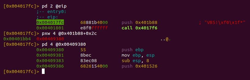
Figure 9.22 – Finding the SubMain address for the VB sample in radare2

Now, let’s talk about the dynamic analysis of Visual Basic samples.

Dynamic analysis

Just like static analysis, a dynamic analysis will be different for p-code and native code samples.

P-code

When there is a need to debug p-code compiled code, generally, there are two options available: debug the p-code instructions themselves or debug the restored source code.

The second option requires a high-quality decompiler that can produce something close to the original source code. Usually, VB Decompiler does this job pretty well. In this case, its output can be loaded into an IDE of your choice and after some minor modifications, it can be used to debug any usual source code. Often, it isn’t necessary to restore the whole project as only certain parts of the code need to be traced.

While this approach is more user-friendly in general, sometimes, debugging actual p-code may be the only option available, for example, when a decompiler doesn’t work properly or just isn’t available. In this case, the WKTVBDE project becomes extremely handy as it allows you to debug p-code compiled applications. It requires a malicious sample to be placed in its root directory to be loaded properly.

Native code

For native code samples, just like for static analysis, dynamic analysis tools for Windows can be used. The choice mainly depends on the analyst’s preferences and available budget.

At this stage, we have learned enough about VB to start analyzing the first few samples. Now, let’s talk about Java-based threats.

The internals of Java samples

Java is a cross-platform programming language that is commonly used to create both local and web applications. Its syntax was influenced by another object-oriented language called Smalltalk. Originally developed by Sun Microsystems and first released in 1995, it later became a part of the Oracle Corporation portfolio. At the time of writing, it is considered to be one of the most popular programming languages in use.

Java applications are compiled into the bytecode that’s executed by Java Virtual Machines (JVMs). The idea here is to let applications that have been compiled once be used across all supported platforms without any changes required. There are multiple JVM implementations available on the market and at the time of writing (starting from Java 1.3), HotSpot JVM is the default official option. Its distinctive feature is its combination of the interpreter and the JIT compiler, which can compile bytecode into native machine instructions based on the profiler output to speed up the execution of slower parts of the code. Most PC users get it by installing the Java Runtime Environment (JRE), which is a software distribution that includes the standalone JVM (HotSpot), the standard libraries, and a configuration toolset. The Java Development Kit (JDK), which also contains JRE, is another popular option since it is a development environment for building applications, applets, and components using the Java language. For mobile devices, the process is quite different. We will cover it in Chapter 13, Analyzing Android Malware Samples.

In terms of malware, Java is quite popular among Remote Access Tool (RAT) developers. Examples include jRAT or the Frutas/Adwind families distributed as JAR files. Exploits used to be another big problem for users until recent changes were introduced by the industry. In this section, we will explore the internals of the compiled Java files and learn how to analyze malware while leveraging it.

File structure

Once compiled, text .java files become .class files and can be executed by the JVM straight away.

Here is their structure according to the official documentation:

ClassFile {
  u4 magic;
  u2 minor_version;
  u2 major_version;
  u2 constant_pool_count;
  cp_info constant_pool[constant_pool_count-1]; 
  u2 access_flags;
  u2 this_class; 
  u2 super_class;
  u2 interfaces_count;
  u2 interfaces[interfaces_count]; 
  u2 fields_count;
  field_info fields[fields_count]; 
  u2 methods_count;
  method_info methods[methods_count]; 
  u2 attributes_count;
  attribute_info attributes[attributes_count];
}

The magic value that’s used in this case is a hexadecimal DWORD, 0xCAFEBABE. The other fields are self-explanatory.

The most common way to release a more complex project is to build a JAR file that contains multiple compiled modules, as well as auxiliary metadata files such as MANIFEST.MF. JAR files follow the usual ZIP archive format and can be extracted using any unpacking software that supports it.

Finally, the Java Network Launch Protocol (JNLP) can be used to access Java files from the web using applets or Java Web Start software (included in the JRE). JNLP files are XML files with certain fields that are expected to be populated. Generally, except for the generic information about the software, it makes sense to pay attention to the <jar> field, which is a reference to the actual JAR file, and the <applet-desc> field, which, among other things, specifies the name of the main Java class to be loaded.

There are numerous ways that Java-based samples can be analyzed. In this section, we are going to explore multiple options available for both static and dynamic analysis.

JVM instructions

The list of supported instructions is very well-documented, so generally, it isn’t a problem to find information about any bytecode of interest. Let’s look at some examples of what they look like.

Data transfer:

Arithmetic and logical operations:

Control flow:

Interestingly enough, other projects can produce Java bytecode, such as JPython, which aims to compile Python files into Java-style bytecode. However, in reality, in the absolute majority of cases, working with them is not necessary as modern decompilers are doing their job extremely well.

Static analysis

Since the Java bytecode remains the same across all platforms, it speeds up the process of creating high-quality decompilers as developers don’t have to spend much time supporting different architectures and operating systems. Here are some of the most popular tools available to the general public:

• Krakatau: This is a set of three tools written in Python that allows you to decompile and disassemble Java bytecode, as well as assemble it. Don’t forget to specify the path to the rt.jar file from your Java folder via the -path argument when using it.
• Procyon: Another powerful decompiler, this can process both Java files and raw bytecode.
• FernFlower: A Java decompiler that’s maintained as a plugin for IntelliJ IDEA. It has a command-line version as well.
• CFR: A JVM bytecode decompiler written in Java that can process individual classes and entire JAR files as well.
• d4j: A Java decompiler built on top of the Procyon project.
• Ghidra: This reverse-engineering toolkit supports multiple file formats and instruction sets, including Java bytecode:

Figure 9.23 – Disassembled and decompiled Java bytecode in Ghidra

• JD Project: A venerable Java decompiler project, this provides a set of tools for analyzing Java bytecode. It includes a library called JD-Core, a standalone tool called JD-GUI, and several plugins for major IDEs.
• JAD: A classic decompiler that has assisted generations of reverse engineers with Java malware analysis. It’s now discontinued:

Figure 9.24 – Decompiled code of the Adwind RAT malware written in Java

It always makes sense to try several different projects and compare their output since all of them implement different techniques, so the quality may vary, depending on the input sample.

To know where to start the analysis, look inside the MANIFEST.MF file as it will indicate from which class of the corresponding JAR sample the execution will start (the Main-Class field).

Finally, if necessary, Java bytecode disassembly can be obtained using a standard javap tool with the -c argument.

Dynamic analysis

Modern decompilers generally produce a reasonably high-quality output, which, after minor modifications, can be read and debugged as any usual Java source code. Multiple IDEs support Java that provide debugging options for this purpose: Eclipse, NetBeans, IntelliJ IDEA, and others.

If the original bytecode tracing is required, it is possible to achieve this with the -XX:+TraceBytecodes option, which is available for debug builds of the HotSpot JVM. If step-by-step bytecode debugging is required, then Dr. Garbage’s Bytecode Visualizer plugin for Eclipse IDE appears to be extremely handy. It allows you to not only see the disassembly of the compiled modules inside the JAR but also debug them.

Dealing with anti-reverse engineering solutions

At the time of writing, there is an impressive number of commercial obfuscators for Java available on the market. As for malware developers, many of them use either cracked versions or demos and leaked licenses. An example is Allatori Obfuscator, which is misused by Adwind RAT.

When the obfuscator’s name is confirmed (for example, by unique strings), it generally makes sense to check whether any of the existing deobfuscation tools support it. Here are some of them:

• Java Deobfuscator: A versatile project that supports a decent amount of commercial protectors
• JMD: A Java bytecode analysis and deobfuscation tool that can remove obfuscation implemented by multiple well-known protectors
• Java DeObfuscator (JDO): A general-purpose deobfuscator that implements several universal techniques, such as renaming obfuscated values to be unique and indicative of their data type
• jrename: Another universal deobfuscator that specializes in renaming values to make the code more readable

If nothing ready-to-use has been found, it makes sense to search for articles covering this particular obfuscator as they may give you valuable insight into how it works and what approach is worth trying.

If no information has been found, then it is time to explore the logic behind the obfuscator from scratch, trying to get the most valuable information first, such as strings and then the bytecode. The more information that can be collected about the obfuscator, the less time will be spent on the analysis itself later.

That’s it for Java-based threats. Now, let’s talk about malware written in Python.

Analyzing compiled Python threats

Python is a high-level general-purpose language that debuted in 1990 and since that time has gone through several development iterations. At the time of writing, there are two branches actively used by the public, Python 2 and Python 3, which are not fully compatible. The language itself is extremely robust and easy to learn, which eventually lets engineers prototype and develop ideas rapidly.

As for why compiled Python is used by malware authors when there are so many other languages, this language is cross-platform, which allows an existing application to be easily ported to multiple platforms. It is also possible to create executables from Python scripts using tools such as py2exe and PyInstaller.

You may be wondering, why is Python being covered in this chapter when it is a scripting language? The truth is, whether the programming language uses bytecode or not depends on the actual implementation and not on the language itself. Active Python users may notice files with the .pyc extension appearing, for example, when the Python modules get imported. These files contain the code that’s been compiled into Python’s bytecode language and can be used for various purposes, including malicious ones. In addition, the executables that are generated from Python projects can generally be reverted to these bytecode modules first.

In this section, we will explain how such samples can be analyzed.

File structure

There are three types of compiled files associated with Python: .pyc, .pyo, and .pyd. Let’s go through the differences between them:

• .pyc: These are standard compiled bytecode files that can be used to make future module importing easier and faster
• .pyo: These are compiled bytecode files that are built with the -O (or -OO) option, which is responsible for introducing optimizations that affect the speed they will be loaded (not executed)
• .pyd: These are traditional Windows DLL files that implement the MZ-PE structure (for Linux, it will be .so)

Since MZ-PE files have been covered multiple times throughout this book, we won’t talk about them too much, nor spend much time on .pyd files. Their main feature is having a specific name for the initialization routine that should match the name of the module.

Particularly, if you have a module named foo.pyd, it should export a function called initfoo so that later, when imported using the import foo statement, Python can search for the module with such a name and know the name of the initialization function to be loaded.

Now, let’s focus on the compiled bytecode files. Here is the structure of the .pyc file:

Interestingly enough, the .pyc modules are platform independent, but at the same time Python version-dependent. Thus, .pyc files can easily be transferred between systems with the same Python version installed, but files that are compiled using one version of Python generally can’t be used by another version of Python, even on the same system.

Bytecode instructions

The official Python documentation describes the bytecode that’s used in both versions 2 and 3. In addition, since it is open source software, all bytecode instructions for a particular Python version can be also found in the corresponding source code files, mainly ceval.c.

The differences between the bytecode that’s used in Python 2 and 3 aren’t that drastic, but still noticeable. For example, some instructions that were implemented for version 2 are gone in version 3 (such as STOP_CODE, ROT_FOUR, PRINT_ITEM, PRINT_NEWLINE/PRINT_NEWLINE_TO, and so on):

Figure 9.25 – Different bytecode for the same HelloWorld script produced by Python 2 and 3

Here are the groups of instructions that are used in the official documentation for Python 3, along with some examples:

• General instructions: Implements the most basic stack-related operations:
  • NOP: Do nothing (generally used as a placeholder)
  • POP_TOP: Removes the top value from the stack
  • ROT_TWO: Swaps the top items on the stack
• Unary operations: These operations take the first item on the stack, process it, and then push it back:
  • UNARY_POSITIVE: Increment
  • UNARY_NOT: Logical NOT operation
  • UNARY_INVERT: Inversion
• Binary operations: For these operations, the top two items are taken from the stack and the result is pushed back:
  • BINARY_MULTIPLY: Multiplication
  • BINARY_ADD: Addition
  • BINARY_XOR: XOR operation
• In-place operations: These instructions are pretty much the same as Binary analogs, with the difference mainly being in the implementation (the operations are done in-place). Examples of such instructions are as follows:
  • INPLACE_MULTIPLY: Multiplication
  • INPLACE_SUBTRACT: Subtraction
  • INPLACE_RSHIFT: Right shift operation
• Coroutine opcodes: Coroutine-related opcodes:
  • GET_AITER: Call the get_awaitable function for the output of the __aiter__() method of the top item on the stack
  • SETUP_ASYNC_WITH: Create a new frame object
• Miscellaneous opcodes: The most diverse category, this contains bytecode for many different types of operations:
  • BREAK_LOOP: Terminate a loop
  • SET_ADD: Add the top item on the stack to the set specified by the second item
  • MAKE_FUNCTION: Push a new function object to the stack

The bytecode instruction names are quite self-explanatory. For the exact syntax, please consult the official documentation.

After discussing the various aspects of Python as a scripting language, we will now pay attention to how to analyze compiled Python code. In this section, we will go through the practical analysis techniques from a Python perspective.

Static analysis

In many cases, the analysts don’t get the compiled Python modules straight away. Instead, they get a sample, which is a set of Python scripts that’s been converted into an executable using either py2exe or PyInstaller solutions. So, before digging into bytecode modules themselves, we need to obtain bytecode modules. Luckily, several projects can perform this task:

• unpy2exe.py: This script can handle samples built using py2exe
• pyinstxtractor.py: As the name suggests, this tool can be used to extract Python modules from the executables built using the PyInstaller solution

An open source project called python-exe-unpacker combines both of these tools and can be run against the executable sample without any extra checks.

After extracting the files that were packed using PyInstaller, there is one moment that can be quite frustrating for anybody who just started analyzing compiled Python files. In particular, the main extracted module may be missing the first few bytes preceding the marshaled code (see the preceding table for the exact number that depends on the Python version), so it can’t be processed by other tools straight away. The easiest way to handle this is to take them from any compiled file on the current machine and then add them there using any hex editor. Such a file can be created by importing (not executing) a simple Hello World script.

Since analyzing Python source code is pretty straightforward, it makes sense to stick to this option where possible. In this case, the decompilers, which can restore the original code, appear to be extremely useful. At the time of writing, multiple options are available:

• uncompyle6: An open source native Python decompiler that supports multiple versions of it. It does exactly what it promises – translates bytecode back into equivalent source code. There were several older projects preceding it (decompyle, uncompyle, and uncompyle2).
• decompyle3: A reworking of the uncompyle6 project that supports Python versions 3.7+
• Decompyle++ (also known as pycdc): A disassembler and decompiler written in C++, it seeks to support bytecode from any version of Python.
• Meta: A Python framework that allows you to analyze Python bytecode and syntax trees.
• UnPYC: A versatile GUI tool for Python decompiling that relies on other projects to do the actual code restoration.

After obtaining the source code, it can be reviewed in any text editor with convenient syntax highlighting or an IDE of your choice.

However, in certain cases, the decompiling process is not possible straight away. For example, when the module was built using the newest version of Python, it became corrupted during a transfer, partial decoding/decryption, or maybe due to some anti-reverse engineering technique. Such tasks can also be found in some CTF competitions. In this case, the engineer has to stick to analyzing the bytecode. Apart from the tools we mentioned previously, the marshal.load and dis.disassemble methods can be used to translate the bytecode into a readable format.

Dynamic analysis

In terms of dynamic analysis, usually, the output of decompilers can be executed straight away. Step-by-step execution is supported by any major IDE that supports the Python language. In addition, step-by-step debugging is possible with the trepan2/trepan3k debugger (for recent versions of Python 2 and 3, respectively), which automatically uses uncompyle6 if there is no source code available. For Python before 2.6, the older packages, pydbgr and pydb, can be used.

If there is a necessity to trace the bytecode, there are several ways it can be handled, as follows:

• Patching the Python source code: In this case, usually, the ceval.c file is amended to process (for example, print) executed instructions.
• Amending the .pyc file itself: Here, the source code line numbers are replaced with the index of each byte, which eventually allows you to trace executed bytecode. Ned Batchelder covered this technique in his Wicked hack: Python bytecode tracing article.

There are also existing projects such as bytecode_tracer that aim to handle this task (at the time of writing, it only supports .pyc files with a header format that’s generated by the current version of Python 2, so update it if necessary).

Some examples of common anti-reverse engineering techniques include doing the following:

• Manipulating non-existing values on the stack
• Setting up a custom exception handler (for this purpose, the SETUP_EXCEPT instruction can be used)

When editing the bytecode (for example, to get rid of anti-debugging or anti-decompiling techniques or to restore a corrupted code block), the dis.opmap mapping appears to be extremely useful to find the binary values of opcodes and later replace them, and the bytecode_graph module can be used to seamlessly remove unwanted values.

Summary

In this chapter, we covered the fundamental theory of bytecode languages. We learned what their use cases are and how they work from the inside. Then, we dived deep into the most popular bytecode languages used by modern malware families, explained how they operate, and looked at their unique specifics that need to be paid attention to. Finally, we provided detailed guidelines on how such malware can be analyzed and the tools that can facilitate this process.

Equipped with this knowledge, you can analyze malware of this kind and get an invaluable insight into how it may affect victims’ systems.

In Chapter 10, Scripts and Macros – Reversing, Deobfuscation, and Debugging, we are going to cover various script and macros languages, explore the malware that misuses them, and find interesting links between them, as well as already covered technologies.