Chapter 8: Reinforcement Learning
The reinforcement learning paradigm is very different than standard machine learning and even the online machine learning methods that we have covered in earlier chapters. Although reinforcement learning will not always be a better choice than "regular" learning for many use cases, it is a powerful tool for tackling re-learning and the adaptation of models.
In reinforcement learning, we give the model a lot of decisive power to do its re-learning and to update the rules of its decision-making process. Rather than letting the model make a prediction and hardcode the action to take for this prediction, the model will directly decide on the action to take.
For automated machine learning pipelines in which actions are effectively automated, this can be a great choice. Of course, this must be complemented with different types of logging, monitoring, and more. For cases in which we need a prediction rather than an action, reinforcement learning will not be appropriate.
Although very powerful in the right use case, reinforcement learning is currently not a standard choice with respect to regular machine learning. In the future, reinforcement learning may very well gain popularity for a larger number of use cases.
In this chapter, you will first be thoroughly introduced to the different concepts behind reinforcement learning. You will then see an implementation of reinforcement learning in Python.
This chapter covers the following topics:
- Defining reinforcement learning
- The main steps of reinforcement learning models
- Exploring Q-learning
- Deep Q-learning
- Using reinforcement learning for streaming data
- Use cases of reinforcement learning
- Implementing reinforcement learning in Python
Technical requirements
You can find all the code for this book on GitHub at the following link: https://github.com/PacktPublishing/Machine-Learning-for-Streaming-Data-with-Python. If you are not yet familiar with Git and GitHub, the easiest way to download the notebooks and code samples is the following:
- Go to the link of the repository.
- Go to the green Code button.
- Select Download zip.
When you download the ZIP file, you unzip it in your local environment, and you will be able to access the code through your preferred Python editor.
Python environment
To follow along with this book, you can download the code in the repository and execute it using your preferred Python editor.
If you are not yet familiar with Python environments, I would advise you to check out either Anaconda (https://www.anaconda.com/products/individual), which comes with the Jupyter Notebook and JupyterLab, which are both great for executing notebooks. It also comes with Spyder and VSCode for editing scripts and programs.
If you have difficulty installing Python or the associated programs on your machine, you can check out Google Colab (https://colab.research.google.com/) or Kaggle Notebooks (https://www.kaggle.com/code), which both allow you to run Python code in online notebooks for free, without any setup.
Note
The code in the book will generally use Colab and Kaggle notebooks with Python version 3.7.13 and you can set up your own environment to mimic this.
Defining reinforcement learning
Reinforcement learning is a subdomain of machine learning that focuses on creating machine learning models that make decisions. Sometimes, the models are not referred to as models, but rather as intelligent agents.
When looking from a distance, you could argue that reinforcement learning is very close to machine learning. We could say that both of them are methods inside artificial intelligence that try to deliver intelligent black boxes, which are able to learn specific tasks just like a human would – often better.
If we look closer, however, we start to see important differences. In previous chapters, you have seen machine learning models such as anomaly detection, classification, and regression. All of them use a number of variables and are able to make real-time predictions on a target variable based on those.
You have seen a number of metrics that allow us data scientists to decide whether a model is any good. The online models are also able to adapt to changing data by relearning and continuously taking into account their own error metrics.
Reinforcement learning goes further than that. RL models not only make predictions but also take action. You could say that offline models do not take any autonomy in relearning from their mistakes, online models do take into account mistakes right away, and reinforcement learning models are designed to make mistakes and learn from them.
Online models can adapt to their mistakes, just like reinforcement learning. However, when you build the first version of an online model, you do expect it to have acceptable performance in the beginning, and you would train it on some historical data. It can then adapt in the case of data drift or other changes.
The reinforcement learning model, on the other hand, starts out totally naïve and unknowing. It will try out actions, make some mistakes, and then by pure hazard at some point, it will make some good decisions as well. At this point, the reinforcement model will receive rewards and start to remember those.
Comparing online and offline reinforcement learning
Reinforcement learning is generally online learning: the intelligent agent learns through repeated action taking with rewards for good predictions. This can continue indefinitely, at least as long as feedback on the decision keeps getting fed into the model.
However, reinforcement learning can also be offline. In this case, the model would learn for a given period of time, and then at some point, the feedback loop is cut off so that the model (the decision rules) stays the same after that point.
In general, when reinforcement learning is used, it is because we are interested in continuous relearning. So, the online variant is the most common.
A more detailed overview of feedback loops in reinforcement learning
Now, let's go more into the details of reinforcement learning. To start, it is important to understand how the feedback loop of a general reinforcement learning model works. The following schema shows the logic of a model learning through a feedback loop.

Figure 8.1 – Feedback loops in RL
In this schema, you observe the following elements:
- The RL agent: Our model that is continuously learning and making decisions.
- The environment: A fixed environment in which the agent can make a specific set of decisions.
- The action: Every time the agent makes a decision, this will alter the environment.
- The reward: If the decision yields a good result, then a reward will be given to the agent.
- The state: The information about the environment that the agent needs to make its decisions.
As a simplified example, imagine that the agent is a human baby learning to walk. At each point in time, the baby is trying out stuff that could get them to walk. More specifically, they are activating several muscles in their body.
While doing this, the baby is observing that they are or are not walking. Also, their parents cheer them on when they are getting closer to walking correctly. This is a reward being sent to the baby that indicates to them that they are learning in the right way.
The baby will then again try to walk by using almost the same muscles, but with a little variation. If it's better, they'll see that as a positive thing and continue to move in that way.
Let's now cover the remaining steps that are necessary for all of this to work.
The main steps of a reinforcement learning model
The actions of the agent are the decisions that it can make. This is a limited set of decisions. As you will understand, the agent is just a piece of code, so all its decisions will need to be programmed controls of its own behavior.
If we think of it as a computer game, then you understand that the actions that you as a player can execute are limited by the buttons that you can press on your game console. All of the combinations together still allow for a very wide range of options, but they are limited in some way.
The same is true for our human baby learning to walk. They only have control over their own body, so they would not be able to execute any actions beyond this. This gives a huge number of things that can be done by humans, but still, it is a fixed set of actions.
Making the decisions
Now, as your reinforcement agent is receiving information about its environment (the state), it will need to convert this information into a decision. This is the same idea as a machine learning model that needs to map independent variables into a target variable.
This decision mapping is generally called the policy in the case of reinforcement learning. The policy will generally decide on the best action by estimating the expected rewards and then executing the action with the highest expected reward.
Updating the decision rules
The last part of this big picture description of reinforcement learning is the update of the policy: basically, the learning itself. There are many models, and they all have their own specificities, but let's try to get a general idea anyway.
At this point, you have seen that an agent takes an action from a set of fixed actions. The agent has estimated which is most likely to maximize rewards. After the execution of this task, the model will receive a certain reward. This will be used to alter the policy, in a way that depends on the exact method of reinforcement learning that you use.
In the next section, you will see how this can be done in more detail by exploring the Q-learning algorithm.
Exploring Q-learning
Although there are many variants of reinforcement learning, the previous explanation should have given you a good general overview of how most reinforcement models work. It is now time to move deeper into a specific model for reinforcement learning: Q-learning.
Q-learning is a reinforcement learning algorithm that is, so-called, model free. Model-free reinforcement learning algorithms can be seen as pure trial-and-error algorithms: they have no prior notion of the environment, but merely just try out actions and learn whether their actions yield the correct outcome.
Model-based algorithms, on the other hand, use a different theoretical approach. Rather than just learning the outcome based on the actions, they try to understand their environment through some form of a model. Once the agent learns how the environment works, it can take actions that will optimize the reward according to this knowledge.
Although the model-based approach may seem more intuitively likely to perform, model-free approaches such as Q-learning are actually quite good.
The goal of Q-learning
The goal of the Q-learning algorithm is to find a policy that maximizes the expected reward obtained from a number of successive steps starting at the current state.
In regular language, this means that Q-learning looks at the current state (the variables of its environment) and then uses this information to take the best steps in the future. The model does not look at past happenings, only the future.
The model uses the Q-value as a calculation for the quality of a state-action combination: that is, for each state, there is a list of potential actions. Each combination of a potential state and a potential action is called a state-action combination. The Q-value indicates the quality of this action when the state is the given one.
At the beginning of the reinforcement learning process, the value of Q is initialized in some way (randomly or fixed) and then updates every time that a reward is received. The agent handles the model according to the Q-values, and when rewards (feedback on the actions) start to come in, those Q values change. The agent still continues to follow the Q-values, but as they update, the behavior of the agent changes.
The core of this algorithm is the Bellman equation: an update rule for Q-values that uses a weighted average of older and new Q-values. Therefore, old information is forgotten at some point, when a lot of learning has happened. This avoids getting "stuck" in previous behaviors.
The formula of the Bellman equation is the following:

Parameters of the Q-learning algorithm
In this Bellman equation, there are a few important parameters that you can tune. Let's briefly cover those:
- The learning rate is a very commonly used hyperparameter in machine learning algorithms. It generally defines the step size of an optimizer in which large steps may make you move around faster in the optimization space, but too large steps may also cause a problem to go into narrow optimums.
- The discount factor is a concept that is very often used in finance and economics. In reinforcement learning, it indicates at which rate the model needs to prioritize short-term or long-term rewards.
After this overview of Q-learning, the next section will introduce a more complex alternative version of this approach called Deep Q-learning.
Deep Q-learning
Now that you have seen the basics of reinforcement learning and the most basic reinforcement learning model, Q-learning, it is time to move on to a more performant and more commonly used model called Deep Q-learning.
Deep Q-learning is a variant of Q-learning in which the Q-values are not just a list of expected Q-values for each combination of state and actions, updated by the Bellman equation. Rather, in Deep Q-learning, this estimation is done using a (deep) neural network.
If you are not familiar, neural networks are a class of machine learning models that are amongst the state of the art in terms of performance. Neural networks are largely used for many use cases in artificial intelligence, machine learning, and data science in general. Deep neural networks are the technology that allows many data science use cases such as Natural Language Processing (NLP), computer vision, and much more.
The idea behind the neural network is to pass an input data point through a network of nodes, called neurons, that each do a very simple operation. The fact that there are many such simple operations being done, and weights applied in between, means that the neural network is a powerful learning algorithm for mapping input data into a target variable.
The following example shows a standard depiction of a neural network. The models can be as simple or as complex as you want. You can go to huge numbers of hidden layers and add as many nodes per hidden layer as you want. Each arrow is a coefficient and needs to be estimated. So, it must be kept in mind that a large quantity of data will be necessary for estimating such models.
The example schematic of a neural network is shown here:
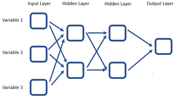
Figure 8.2 – Neural network architecture
For reinforcement learning, this has to be applied inside the Q-learning paradigm. In essence, the deep learning model is just a better way to estimate Q-values than the standard Q-learning approach (or at least that's what it aspires to be).
You could see the analogy as follows. In standard Q-learning, there is a relatively simple storage and update mechanism for new rewards coming in and updating the policy. You could see it as depicted as a table, as follows:
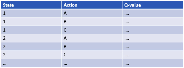
Figure 8.3 – Example table format
In Deep Q-learning, the input and output processes are mostly the same, yet the state is transcribed as a number of variables that are input into a neural network. The neural network then outputs the estimated Q-values for each action.
The following graph shows how the state is added as input to the neural network.

Figure 8.4 – Adding the state as input to the neural network
Now that you understand the theory behind reinforcement learning, the next section will be more applied as it presents a number of example use cases for reinforcement learning on streaming data.
Using reinforcement learning for streaming data
As discussed throughout earlier chapters, the challenge of building models on streaming data is to find models that are able to learn incrementally and that are able to adapt in the case of model drift or data drift.
Reinforcement learning is a potential candidate that could respond well to those two challenges. After all, reinforcement learning has a feedback loop that allows it to change policy when many mistakes are made. It is therefore able to adapt itself in the event of changes.
Reinforcement learning can be seen as a subcase of online learning. At the same time, the second specificity of reinforcement learning is its focus on learning actions, whereas regular online models are focused on making accurate predictions.
The split between the two fields is present in practice in the types of use cases and domains of application, but many streaming use cases have the potential to benefit from reinforcement learning and it is a great toolset to master.
If you are looking for more depth and examples, you can look at the following insightful article: https://www.researchgate.net/publication/337581742_Machine_learning_for_streaming_data_state_of_the_art_challenges_and_opportunities.
In the next section, we will explore a few key use cases where reinforcement learning proves crucial.
Use cases of reinforcement learning
The use cases of reinforcement learning are almost as numerous as online learning. It is a less often used technology when compared to standard offline and online models, but with the changes in the machine learning domain over the last years, it is still a great candidate that could become huge in the coming years.
Let's look at some use cases to get a better feel of the types of use cases that can be suitable for reinforcement learning. Among the types of examples, there are some that are more traditional reinforcement learning use cases, and others that are more specific streaming data use cases.
Use case one – trading system
As a first use case of reinforcement learning, let's talk about stock market trading. The stock market use case was already discussed in the forecasting use case of the regression chapter. Reinforcement learning is an alternative solution to it.
In regression, online models are used to build forecasting tools. Using these forecasting tools, a stock trader could predict the price developments of specific stocks in the near future and use those predictions to decide on buying or selling the stocks.
Using reinforcement learning, the use case would be developed slightly differently. The intelligent agent would learn how to make decisions rather than to predict prices. As an example, you could give the agent three actions: sell, buy, or hold (hold meaning do nothing/ignore).
The agent would receive information about its environment, which could include past stock prices, macroeconomic information, and much more. This information would be used together with a policy and this policy decides when to buy, sell, or hold.
By training this agent for a long period of time, and with a lot of data including all types of market scenarios, the agent could learn pretty well how to trade markets. You would then obtain a profitable "trading robot," making money without much intervention. If successful, this is clearly an advantage over regression models as they only predict price and do not take any action.
For more information on this topic, you could start by checking out the following links:
- https://arxiv.org/pdf/1911.10107.pdf
- http://cslt.riit.tsinghua.edu.cn/mediawiki/images/a/aa/07407387.pdf
Use case two – social network ranking system
A second use case for reinforcement learning is the ranking of posts on social networks. The general idea of what happens behind this is a number of posts being created and the most relevant has to be shown to each specific user, based on their preference.
There are many machine learning approaches that could be leveraged for this, and reinforcement learning is one of them. Basically, the model would end up making decisions on the posts to show to the user, so in this way, it is a real action that is taken.
This action also generates feedback. If the user likes, comments, shares, clicks, pauses, or interacts in other ways with the post, the agent will be rewarded and learns that this type of post does interest the user.
By trial and error, the agent can publish different types of posts to each user and learn which decisions are good and which are bad.
Real-time response is very important here, as well as learning rapidly from mistakes. If a user receives a number of irrelevant posts, this would be detrimental to their user experience and the model should learn as soon as possible that its predictions are not correct. Online learning or reinforcement learning is therefore great for this use case.
For more information about such use cases, you can find some materials here:
- https://arxiv.org/abs/1601.00667
- https://rbcdsai.iitm.ac.in/blogs/finding-influencers-in-social-networks-reinforcement-learning-shows-the-way/
Use case three – a self-driving car
Reinforcement learning has also been proposed for the use case of self-driving cars. As you probably know, self-driving cars have been increasingly gaining attention over the last few years. The goal is to make machine learning or artificial intelligence models that can replace the behavior of human drivers.
It is easy to understand that the essential part of this model will be to take actions: accelerate, slow down, brake, turn, and so on. If a good enough reinforcement learning model could be built to obtain all those skills, it would be a great candidate for building self-driving cars.
Self-driving cars need to respond to a large stream of data about the environment. For example, they need to detect cars, roads, road signs, and much more on a continuous video stream that is being filmed on multiple cameras, together with other sensors potentially.
Real-time responses are key in this scenario. Retraining the model in real time might be more problematic, as you would want to make sure that the model is not applying a trial-and-error methodology while on the road.
More information on this can be found at the following links:
- https://arxiv.org/ftp/arxiv/papers/1901/1901.00569.pdf
- https://www.ingentaconnect.com/contentone/ist/ei/2017/00002017/00000019/art00012?crawler=true&mimetype=application/pdf
Use case four – chatbots
Another very different but also very advanced use case of machine learning is the development of chatbots. Intelligent chatbots are still rare, but we can expect to see chatbots become more intelligent in the near future.
Chatbots need to be able to generate a response to a person while treating the information that was given to it by a user. The chatbot is therefore performing a sort of action: replying to the human.
Reinforcement learning in combination with other techniques from the domain of natural language processing can be a good solution for such problems. By letting the chatbot talk with users, a reward can be given by the human user in the form of, for example, an evaluation of the usefulness of their interaction. This reward can then help the reinforcement learning agent adapt its policy and make replies more appropriate in future interactions.
Chatbots need to be able to respond in real time, as no one wants to wait for an answer from a chatbot interaction. Learning can be done in an online or an offline fashion, but reinforcement learning is definitely one of the suitable alternatives.
You can read more on this use case here:
Use case five – learning games
As a final use case example for reinforcement learning, let's talk about the use case of learning games. It may be less valuable for business, but it is still an interesting use case of reinforcement learning.
Over the past years, reinforcement learning agents have learned to play a number of games, including chess and Go. There is a clear set of moves that can be made at each step, and by playing many simulated (or real) games, the models can learn which policy (decision rules for the step to take) are the best.
In the end, the agent has such a powerful policy that it can often beat the best human players in the world at such games.
You can find more examples of this at the following links:
Now that we have explored some of the use cases for reinforcement learning, let's implement it using Python, in the next section.
Implementing reinforcement learning in Python
Let's now move on to an example in which streaming data is used for Q-Learning. The data that we will be using is simulated data of stock prices:
- The data is generated in the following block of code.
The list of values that is first generated is a list of 30,000 consecutive values that represent stock prices. The data generating process is the starting point of 0 and at every time step, there is a random value added to this. The random normal values are centered around 0, which indicates that prices would go up or down by a step size based on a standard deviation of 1.
This process is often referred to as a random walk and it can go quite far up or down. After that, the values are standardized to be within a normal distribution again.
Code Block 8-1
import numpy as np
import matplotlib.pyplot as plt
import random
starting = 0
values = [starting]
for i in range(30000):
values.append(values[-1] + np.random.normal())
values = (values - np.mean(values)) / np.std(values)
plt.plot(values)
The resulting plot can be seen in the following:
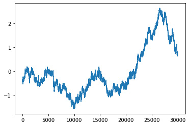
Figure 8.5 – The resulting plot from the preceding code block
- Now, for a reinforcement problem, it is necessary to have a finite number of states. Of course, if we consider stock prices, we could collect up to an infinite number of decimals. The data is rounded to 1 decimal to limit the number of possible state data points:
Code Block 8-2
rounded_values = []
for value in values:
rounded_values.append(round(value, 1))
plt.plot(rounded_values)
The resulting graph is shown in the following figure:

Figure 8.6 – The graph resulting from the preceding code block
- We can now set the states' potential values to all of the values that have happened in the past. We can also initiate a policy.
As seen in the theoretical part of this chapter, the policy represents the rules of the reinforcement learning agent. In some cases, there is a very specific ruleset, but in Q-learning, there is only a Q-value (quality) for each combination of state and action.
In our example, let's consider a stock trading bot that can only do two things at a time t. Either the trading bot buys at time t and sells at t+1, or it sells at time t and closes the sell position at time t+1. Without going into stock trading too much, the important things to understand about this are the following:
- When the agent buys, it should do so because it expects the stock market to go up.
- When the agent opens a sell order, it should do so because it expects the stock market to go down.
As information, our stock trader will be very limited. The only data point in the state is the price at time t. The goal here is not to make a great model, but to show the principles of building a reinforcement learning agent on a stock trading example. In reality, you'd need much more information in the state to decide on your action:
Code Block 8-3
states = set(rounded_values)
import pandas as pd
policy = pd.DataFrame(0, index=states, columns=['buy', 'sell'])
- The function defined hereafter is how to obtain an action (sell or buy) based on the Q-table. It is not entirely correct to refer to the Q table as the policy, but it does make it more understandable.
The action chosen is that with the highest Q value for a given state (state is the current value of the stock):
Code Block 8-4
def find_action(policy, current_value):
if policy.loc[current_value,:].sum() == 0:
return random.choice([ 'buy', 'sell'])
return policy.columns[policy.loc[current_value,:].argmax()]
- It is also necessary to define an update rule. In this example, the update rule is based on the Bellman equation that was explained earlier on. However, keep in mind that the agent is fairly simple, and the discounting part is not really relevant. Discounting is useful to make an agent prefer short-term gains over long-term gains. The current agent always makes its gains in one time step, so discounting is of no added value. In a real stock-trading bot, this would be very important: you wouldn't put your money on a stock that will double over 20 years if you could double it in 1 year instead:
Code Block 8-5
def update_policy(reward, current_state_value, action):
LEARNING_RATE = 0.1
MAX_REWARD = 10
DISCOUNT_FACTOR = 0.05
return LEARNING_RATE * (reward + DISCOUNT_FACTOR * MAX_REWARD - policy.loc[current_state_value,action])
- We now get to the execution of the model. We start by setting past_state to 0 and past_action to buy. The total reward is initialized at 0 and an accumulator list for rewards is instantiated.
The code will then loop through the rounded values. This is a process that copies a data stream. If the data arrived one by one, the agent would be able to learn in exactly the same manner. The essence is an update of the Q table at every learning step.
Within each iteration, the model will execute the best action, where the best is based on the Q values of the Q values table (policy). The model will also receive the reward from time step t-1, as this was defined as the only option for the stock trading bot. Those rewards will be used to update the Q table so that the next round can have updated information:
Code Block 8-6
past_state_value = 0
past_action = 'buy'
total_reward = 0.
rewards = []
for i, current_state_value in enumerate(rounded_values):
# do the action
action = find_action(policy, current_state_value)
# also compute reward from previous action and update state
if past_action == 'buy':
reward = current_state_value - past_state_value
if past_action == 'sell':
reward = past_state_value - current_state_value
total_reward = total_reward + float(reward)
policy.loc[current_state_value, action] = policy.loc[current_state_value, action] + update_policy(reward, current_state_value,action)
#print(policy)
rewards.append(total_reward)
past_action = action
past_state_value = current_state_value
- In the following plot, you see how the model is getting its rewards. In the beginning, total rewards are negative for a long time, and then they are positive at the end. Keep in mind that we are learning on input data that is hypothetical and that represents a random walk. If we wanted an actual intelligent stock trading bot, we'd need to give it much more and much better data:
Code Block 8-7
plt.plot(rewards)
The resulting graph is shown hereafter:

Figure 8.7 – The graph resulting from the preceding code block
- The following plot shows a heat map of the Q values against the policy. The values at the top of the table are the preferred action when stock prices are low, and the values at the bottom are preferred actions when stock prices are high. The color light yellow means high-quality actions, and the color black means low-quality actions:
Code Block 8-8
import seaborn as sns
sns.heatmap(policy.sort_index())
The resulting heatmap is shown here:
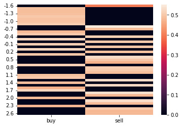
Figure 8.8 – The heatmap resulting from the preceding code block
It is interesting to see that the model seems to have started to learn a basic rule in stock trading: buy low, sell high. This can be seen by more yellow in selling at high prices and more yellow in buying at low prices. Apparently, this rule is even true on simulated random walk data.
To learn more advanced rules, the agent would need to have more data in the state, and therefore the Q table would also become much heavier. An example of what you could add is a rolling history of prices so that the agent knows whether you are in an uptrend or a downtrend. You could also add macro-economic factors, sentiment estimations, or any other data.
You could also make the action structure much more advanced. Rather than having only one-day sell or buy trades, it would be much more interesting to have a model that can buy or sell any equity in its portfolio at any time that the agent decides to.
Of course, you would also need to provide enough data to allow the model to make estimations for all these scenarios. The more scenarios you take into account, the more time it will take the agent to learn how to behave correctly.
Summary
In this chapter, you were first introduced to the underlying foundations of reinforcement learning. You saw that reinforcement learning models are focused on taking actions rather than on making predictions.
You also saw two widely known algorithms for reinforcement learning. This started with Q-learning, which is the foundational algorithm of reinforcement learning, and its more powerful improvement, Deep Q-learning.
Reinforcement learning is often used for more advanced use cases such as chatbots or self-driving cars, but can also be used for numerical data streams very well. Through a use case, you saw how to apply reinforcement learning to streaming data for finance.
With this chapter, you have come to the end of discovering the most relevant machine learning models for online learning. In the coming chapters, you will discover a number of additional tools that you will need to take into account in online learning and that have no real counterpart in traditional ML. You will first have a deep dive into all types of data and model drift and then discover how to deal with models that go totally in the wrong direction through catastrophic forgetting.
Further reading
- Reinforcement learning applications: https://neptune.ai/blog/reinforcement-learning-applications
- Q-learning: https://en.wikipedia.org/wiki/Q-learning
- Deep Q-learning: https://en.wikipedia.org/wiki/Deep_reinforcement_learning