Chapter 7: Online Regression
After looking at online anomaly detection and online classification throughout the previous chapters, there is one large category of online machine learning that remains to be seen. Regression is the family of supervised machine learning models that applies to use cases in which the target variable is numerical.
In anomaly detection and classification, you have seen how to build models to predict categorical targets (yes/no and iris species), but you have not yet seen how to work with a target that is numerical. Working with numerical data requires having methods that work differently, both in the deeper layers of model training and model definition and also in our use of metrics.
Imagine being a weather forecaster trying to forecast the temperature (Celsius) for tomorrow. Maybe you expect a sunny day, and you have a model that you use to predict a temperature of 25 degrees Celsius. Imagine if the next day, you observe that it is cold and only 18 degrees; you were clearly wrong.
Now, imagine that you predicted 24 degrees. In a classification use case, you may tend to say that 25 is not 24, so the result is wrong. However, the result of 24 is less wrong than the result of 18.
In regression, one single prediction can be more or less wrong. In practice, you will rarely be entirely right. In classification, you are either wrong or right, so this is different. This introduces a need for new metrics and a change in the model benchmarking process.
In this chapter, you will first get a deeper introduction to regression models, focusing on online regression models in River. After that, you'll be working on a regression model benchmark.
This chapter covers the following topics:
- Defining regression
- Use cases of regression
- Overview of regression algorithms in River
Technical requirements
You can find all the code for this book on GitHub at the following link: https://github.com/PacktPublishing/Machine-Learning-for-Streaming-Data-with-Python. If you are not yet familiar with Git and GitHub, the easiest way to download the notebooks and code samples is the following:
- Go to the link of the repository.
- Go to the green Code button.
- Select Download ZIP.
When you download the ZIP file, unzip it in your local environment, and you will be able to access the code through your preferred Python editor.
Python environment
To follow along with this book, you can download the code in the repository and execute it using your preferred Python editor.
If you are not yet familiar with Python environments, I would advise you to check out Anaconda (https://www.anaconda.com/products/individual), which comes with Jupyter Notebook and JupyterLab, which are both great for executing notebooks. It also comes with Spyder and VS Code for editing scripts and programs.
If you have difficulty installing Python or the associated programs on your machine, you can check out Google Colab (https://colab.research.google.com/) or Kaggle Notebooks (https://www.kaggle.com/code), which both allow you to run Python code in online notebooks for free, without any setup required.
Defining regression
In this chapter, you will discover regression. Regression is a supervised machine learning task in which a model is constructed that predicts or estimates a numerical target variable based on numerical or categorical independent variables.
The simplest type of regression model is linear regression. Let's consider a super simple example of how a linear regression could be used for regression.
Imagine that we have a dataset in which we have observations of 10 people. Based on the number of hours they study per week, we have to estimate their average grade (on a 1 to 10 scale). Of course, this is a strongly oversimplified problem.
The data looks as follows:
Code Block 7-1
import pandas as pd
nb_hrs_studies = [1, 2, 3, 4, 5, 6, 7, 8, 9, 10]
avg_grade = [5.5, 5.8, 6.8, 7.2, 7.4, 7.8, 8.2, 8.8, 9.3, 9.4]
data = pd.DataFrame({'nb_hrs_studies': nb_hrs_studies, 'avg_grade': avg_grade})data
You will obtain the following data frame:

Figure 7.1 – The dataset
Let's plot the data to see how this can be made into a regression problem:
Code Block 7-2
import matplotlib.pyplot as plt
plt.scatter(data['nb_hrs_studies'], data['avg_grade'])
plt.xlabel('nb_hrs_studies')plt.ylabel('avg_grades')This results in the following output:
Figure 7.2 – A scatter plot of the data
Now, the goal of linear regression is to fit the line (or hyperplane) that best goes through these points and is able to predict an estimated avg_grades for any nb_hrs_studies. Other regression models each have their specific way to construct the prediction function, but eventually have the same goal: creating the best fitting formula to predict a numerical target variable using one or more independent variables.
In the next section, you'll discover some example use cases in which regression can be used.
Use cases of regression
The use cases of regression are huge: it is a very commonly used method in many projects. Still, let's see some examples to get a better idea of the different types of use cases that can benefit from regression models.
Use case 1 – Forecasting
A very common use case for regression algorithms is forecasting. In forecasting, the goal is to predict future values of a variable that is measured over time. Such variables are called time series. Although a number of specific methods exist for time series modeling, regression models are also great contenders for obtaining good performance on future prediction performance.
In some forecasting use cases, real-time responses are very important. An example is stock trading, in which the datapoints of stock prices arrive at a huge velocity and forecasts have to be adapted straight away to use the best possible information for stock trades. Even automated stock trading algorithms exist, and they need to react fast in order to make the most profit on their trades as possible.
For further reading on this topic, you could start by checking out the following links:
- https://www.investopedia.com/articles/financial-theory/09/regression-analysis-basics-business.asp
- https://www.mathworks.com/help/econ/time-series-regression-vii-forecasting.html
Use case 2 – Predicting the number of faulty products in manufacturing
The second example of real-time and streaming regression models being used in practice is the application of predictive maintenance models in manufacturing. For example, you could use a real-time prediction of the number of faulty products per hour in a production line. This would be a regression model as well, as the outcome is a number rather than a categorical variable.
The production line could use this prediction for a real-time alerting system, for example, once a threshold of faulty products is predicted to be reached. Real-time data integration is important for this, as having the wrong products being produced is a large waste of resources.
The following two resources will allow you to read more about this use case:
- https://www.sciencedirect.com/science/article/pii/S2405896316308084
- https://www.researchgate.net/publication/315855789_Regression_Models_for_Lean_Production
Now that we have explored some use cases of regression, let's get started with the various algorithms that we have for regression.
Overview of regression algorithms in River
There is a large number of online regression models available in the River online machine learning package.
A selection of relevant ones are as follows:
- LinearRegression
- HoeffdingAdaptiveTreeRegressor
- SGTRegressor
- SRPRegressor
Regression algorithm 1 – LinearRegression
Linear regression is one of the most basic regression models. A simple linear regression is a regression model that fits a straight line through the datapoints. The following graph illustrates this:

Figure 7.3 – A linear model in a scatter plot
This orange line is a result of the following formula:

Here, y represents avg_grades and x represents nb_hrs_studies. When fitting the model, the a and b coefficients are estimates. The b coefficient in this formula is called the intercept. It indicates the value of y when x equals 0. The a coefficient represents the slope of the line. For each additional step in x, a indicates the amount that is added to y.
This is a version of linear regression, but there is also a version called multiple linear regression, in which there are multiple x variables. In this case, the model does not represent a line but rather a hyperplane, in which a slope coefficient is added for each additional x variable.
Linear regression in River
Let's now move on to build an example of online linear regression using River ML in Python:
- If you remember from the previous example, we used a function called make_classification from scikit-learn. The same can be done for regression problems using make_regression:
Code Block 7-3
from sklearn.datasets import make_regression
X,y = make_regression(n_samples=1000,n_features=5,n_informative=5,noise=100)
- To get a better idea of what has resulted from this make_regression function, let's inspect X of this dataset. You can use the following code to get a quick overview of the data:
Code Block 7-4
pd.DataFrame(X).describe()
The describe() method will put out a data frame with descriptive statistics of the variables, as follows:

Figure 7.4 – Descriptive statistics
There are five columns in the X data, and there are 1,000 observations.
- Now, to look at the y variable, also called the target variable, we can make a histogram as follows:
Code Block 7-5
pd.Series(y).hist()
The resulting histogram can be seen in the following figure:

Figure 7.5 – The resulting histogram
There is much more exploratory data analysis that could be done here, but that would be out of scope for this book.
- Let's now move on to the creation of a train and test set to create a fair model validation approach. In the following code, you can see how to create the train_test_split function from scikit-learn to create a train-test split:
Code Block 7-6
from sklearn.model_selection import train_test_split
X_train, X_test, y_train, y_test = train_test_split(X, y, test_size=0.33, random_state=42)
- You can create the linear regression in River using the following code:
Code Block 7-7
!pip install river
from river.linear_model import LinearRegression
model = LinearRegression()
- This model then has to be fitted to the training data. We use the same loop as you have seen earlier on in the book. This loop goes through the individual datapoints (X and y) and converts the X values into a dictionary, as required by River. The model is then updated datapoint by datapoint using the learn_one method:
Code Block 7-8
# fit the model
for x_i,y_i in zip(X_train,y_train):
x_json = {'val'+str(i): x for i,x in enumerate(x_i)}
model.learn_one(x_json,y_i)
- Once the model has learned from the training data, it needs to be evaluated on the test set. This can be done by looping through the test data and making a prediction for the X values of each datapoint. The y values are stored in a list for evaluation against the actual y values of the test dataset:
Code Block 7-9
# predict on the test set
import pandas as pd
preds = []
for x_i in X_test:
x_json = {'val'+str(i): x for i,x in enumerate(x_i)}
preds.append(model.predict_one(x_json))
- We can now compute the metric of our choice for this regression model, for example, the r2 score. This can be done using the following code:
Code Block 7-10
# compute accuracy
from sklearn.metrics import r2_score
r2_score(y_test, preds)
The obtained result is 0.478.
Let's find out whether other models are more performant at this task in the next section.
Regression algorithm 2 – HoeffdingAdaptiveTreeRegressor
The second online regression model that we'll cover is a much more specific model for online regression. Whereas the LinearRegression model, just like many other models, is an online adaptation of an essentially offline model, many other models are developed specifically for online models. HoeffdingAdaptiveTreeRegressor is one of those.
The Hoeffding Adaptive Tree regressor (HATR) is a regression model that is based on the Hoeffding Adaptive Tree Classifier (HATC). HATC is a tree-based model that uses the adaptive windowing (ADWIN) methodology to monitor the performance of the different branches of a tree. The HATC methodology replaces the branches with new branches when their time is due. This is determined by observing the better performance of the new branches by the old branches. HATC is also available in River.
The HATR regression version is based on the HATC approach and uses an ADWIN concept-drift detector at each decision node. This allows the method to detect possible changes in the underlying data, which is called drift. Drift detection will be covered in more detail in a further chapter.
HoeffdingAdaptiveTreeRegressor in River
We will check out an example as follows:
Code Block 7-11
from river.tree import HoeffdingAdaptiveTreeRegressor
model = HoeffdingAdaptiveTreeRegressor(seed=42)
# fit the model
for x_i,y_i in zip(X_train,y_train):
x_json = {'val'+str(i): x for i,x in enumerate(x_i)}
model.learn_one(x_json,y_i)
# predict on the test set
import pandas as pd
preds = []
for x_i in X_test:
x_json = {'val'+str(i): x for i,x in enumerate(x_i)}
preds.append(model.predict_one(x_json))
# compute accuracy
from sklearn.metrics import r2_score
r2_score(y_test, preds)
- This model obtains an r2 score that is a little worse than the linear regression: 0.437. Let's see if we can do something to make it work better. Let's write a grid search to see whether a number of hyperparameters can help to improve the model.
For this, let's write the model as a function that takes values for the hyperparameters and that returns the r2 score:
Code Block 7-12
def evaluate_HATR(grace_period, leaf_prediction, model_selector_decay):
# model pipeline
model = (
HoeffdingAdaptiveTreeRegressor(
grace_period=grace_period,
leaf_prediction=leaf_prediction,
model_selector_decay=model_selector_decay,
seed=42)
)
# fit the model
for x_i,y_i in zip(X_train,y_train):
x_json = {'val'+str(i): x for i,x in enumerate(x_i)}
model.learn_one(x_json,y_i)
# predict on the test set
preds = []
for x_i in X_test:
x_json = {'val'+str(i): x for i,x in enumerate(x_i)}
preds.append(model.predict_one(x_json))
# compute accuracy
return r2_score(y_test, preds)
Code Block 7-13
grace_periods=[0,5,10,]
leaf_predictions=['mean','adaptive']
model_selector_decays=[ 0.3, 0.8, 0.95]
Code Block 7-14
results = []
i = 0
for grace_period in grace_periods:
for leaf_prediction in leaf_predictions:
for model_selector_decay in model_selector_decays:
print(i)
i = i+1
results.append([grace_period, leaf_prediction, model_selector_decay,evaluate_HATR(grace_period, leaf_prediction, model_selector_decay)])
- The results can then be obtained as follows:
Code Block 7-15
pd.DataFrame(results, columns=['grace_period', 'leaf_prediction', 'model_selector_decay', 'r2_score' ]).sort_values('r2_score', ascending=False)
The obtained result is slightly disappointing, as none of the tested values were able to generate a better result. Unfortunately, this is part of data science, as not all models work well on each use case.

Figure 7.6 – The resulting output of Code Block 7-15
Let's move on to the next model and see whether it fits better.
Regression algorithm 3 – SGTRegressor
SGTRegressor is a stochastic gradient tree for regression. It is another decision tree-based model that can learn with new data arriving. It is an incremental decision tree that minimizes the mean squared error by minimizing the loss function.
SGTRegressor in River
We'll check this out using the following example:
Code Block 7-16
from river.tree import SGTRegressor
# model pipeline
model = SGTRegressor()
# fit the model
for x_i,y_i in zip(X_train,y_train):
x_json = {'val'+str(i): x for i,x in enumerate(x_i)}
model.learn_one(x_json,y_i)
# predict on the test set
preds = []
for x_i in X_test:
x_json = {'val'+str(i): x for i,x in enumerate(x_i)}
preds.append(model.predict_one(x_json))
# compute accuracy
r2_score(y_test, preds)
- The result is worse than the previous models, as it is 0.07. Let's again see whether it can be optimized using hyperparameter tuning:
Code Block 7-17
from river.tree import SGTRegressor
def evaluate_SGT(delta, lambda_value, grace_period):
# model pipeline
model = SGTRegressor(delta=delta,
lambda_value=lambda_value,
grace_period=grace_period,)
# fit the model
for x_i,y_i in zip(X_train,y_train):
x_json = {'val'+str(i): x for i,x in enumerate(x_i)}
model.learn_one(x_json,y_i)
# predict on the test set
preds = []
for x_i in X_test:
x_json = {'val'+str(i): x for i,x in enumerate(x_i)}
preds.append(model.predict_one(x_json))
# compute accuracy
return r2_score(y_test, preds)
Code Block 7-18
grace_periods=[0,10,25]
lambda_values=[0.5, 0.8, 1.]
deltas=[0.0001, 0.001, 0.01, 0.1]
Code Block 7-19
results = []
i = 0
for grace_period in grace_periods:
for lambda_value in lambda_values:
for delta in deltas:
print(i)
i = i+1
result = evaluate_SGT(delta, lambda_value, grace_period)
print(result)
results.append([delta, lambda_value, grace_period,result])
Code Block 7-20
pd.DataFrame(results, columns=['delta', 'lambda_value', 'grace_period', 'r2_score' ]).sort_values('r2_score', ascending=False)
The result is shown in the following:
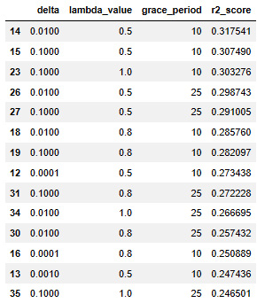
Figure 7.7 – The resulting output of Code Block 7-20
The result is better than the non-tuned SGTRegressor, but much worse than the previous two models. The model could be optimized further, but it does not seem the best go-to for the current data.
Regression algorithm 4 – SRPRegressor
SRPRegressor, or Streaming Random Patches regressor, is an ensemble method that trains an ensemble of base learners on subsets of the input data. These subsets are called patches and are both subsets of features and subsets of observations. This is the same approach as the random forest that was seen in the previous chapter.
SRPRegressor in River
We will check this out using the following example:
- In this example, let's use linear regression as a base learner, as this model has had the best performance compared to the other models tested in this chapter:
Code Block 7-21
from river.ensemble import SRPRegressor
# model pipeline
base_model = LinearRegression()
model = SRPRegressor(
model=base_model,
n_models=3,
seed=42
)
# fit the model
for x_i,y_i in zip(X_train,y_train):
x_json = {'val'+str(i): x for i,x in enumerate(x_i)}
model.learn_one(x_json,y_i)
# predict on the test set
preds = []
for x_i in X_test:
x_json = {'val'+str(i): x for i,x in enumerate(x_i)}
preds.append(model.predict_one(x_json))
# compute accuracy
r2_score(y_test, preds)
- The resulting score is 0.34. Let's try and tune the number of models used to see whether this can improve performance:
Code Block 7-22
def evaluate_SRP(n_models):
# model pipeline
base_model = LinearRegression()
model = SRPRegressor(
model=base_model,
n_models=n_models,
seed=42
)
# fit the model
for x_i,y_i in zip(X_train,y_train):
x_json = {'val'+str(i): x for i,x in enumerate(x_i)}
model.learn_one(x_json,y_i)
# predict on the test set
preds = []
for x_i in X_test:
x_json = {'val'+str(i): x for i,x in enumerate(x_i)}
preds.append(model.predict_one(x_json))
# compute accuracy
return r2_score(y_test, preds)
- You can execute the tuning loop with the following code:
Code Block 7-23
results = []
for n_models in range(1, 50):
results.append([n_models, evaluate_SRP(n_models)])
Code Block 7-24
pd.DataFrame(results,columns=['n_models', 'r2_score']).sort_values('r2_score', ascending=False)
The result is shown in the following:
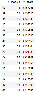
Figure 7.8 – The resulting output of Code Block 7-24
Apparently, the result at 12 models has found a sweet spot at which the performance is 0.457. Compared to the simple LinearRegression model with a score of 0.478, this is a worse result. This indicates that the LinearRegression model has the best score of the four models tested in this dataset.
Of course, this result is strongly related to the data-generating process that is behind the make_regression function. If the make_regression function were to add anything such as time trends, the adaptive models would probably have been more performant than the simple linear model.
Summary
In this chapter, you have seen the basics of regression modeling. You have learned that there are some similarities between classification and anomaly detection models, but that there are also some fundamental differences.
The main difference in regression is that the target variables are numeric, whereas they are categorical in classification. This introduces a difference in metrics, but also in the model definition and the way the models work deep down.
You have seen several traditional, offline regression models and their adaptation to working in an online training manner. You have also seen some online regression models that are made specifically for online training and streaming.
As in the previous chapters, you have seen how to implement a modeling benchmark using a train-test set. The field of ML does not stop evolving, and newer and better models are published regularly. This introduces the need for practitioners to be solid in their skills to evaluate models.
Mastering model evaluation is often even more important than knowing the largest list of models. You need to know a large number of models to start modeling, but it is the evaluation that will allow you to avoid pushing erroneous or overfitted models into production.
Although this is generally true for ML, the next chapter will introduce a category of models that has a fundamentally different take on this. Reinforcement learning is a category of online ML in which the focus is on model updating. Online models have the capacity to learn on each piece of data that gets into the system as well, but reinforcement learning is focused even more on having almost autonomous learning. This will be the scope of the next chapter.
Further reading
- LinearRegression: https://riverml.xyz/latest/api/linear-model/LinearRegression/
- Make_regression: https://scikit-learn.org/stable/modules/generated/sklearn.datasets.make_regression.html
- HoeffdingAdaptiveTreeRegressor: https://riverml.xyz/latest/api/tree/HoeffdingAdaptiveTreeRegressor/
- HoeffdingAdaptiveTreeClassifier: https://riverml.xyz/latest/api/tree/HoeffdingAdaptiveTreeClassifier/
- Adaptive learning and mining for data streams and frequent patterns: https://dl.acm.org/doi/abs/10.1145/1656274.1656287
- SGTRegressor: https://riverml.xyz/latest/api/tree/SGTRegressor/
- SRPRegressor: https://riverml.xyz/latest/api/ensemble/SRPRegressor/