By referring to the following steps, you will be able to project a color image into a reduced color palette using k-means clustering:

1. Now, let's reduce the 16 million colors to a mere 16 by indicating k-means to cluster all of the 16 million color variations into 16 distinct clusters. We will use the previously mentioned procedure, but now define 16 as the number of clusters:

In [9]: criteria = (cv2.TERM_CRITERIA_EPS + cv2.TERM_CRITERIA_MAX_ITER,
...                 10, 1.0)
...     flags = cv2.KMEANS_RANDOM_CENTERS
...     img_data = img_data.astype(np.float32)
...     compactness, labels, centers = cv2.kmeans(img_data,
...                                               16, None, criteria,
...                                               10, flags)

2. The 16 different colors of your reduced color palette correspond to the resultant clusters. The output from the centers array reveals that all colors have three entries—B, G, and R—with values between 0 and 1:

In [10]: centers
Out[10]: array([[ 0.29973754,  0.31500012,  0.48251548],
                [ 0.27192295,  0.35615689,  0.64276862],
                [ 0.17865284,  0.20933454,  0.41286203],
                [ 0.39422086,  0.62827665,  0.94220853],
                [ 0.34117648,  0.58823532,  0.90196079],
                [ 0.42996961,  0.62061119,  0.91163337],
                [ 0.06039202,  0.07102439,  0.1840712 ],
                [ 0.5589878 ,  0.6313886 ,  0.83993536],
                [ 0.37320262,  0.54575169,  0.88888896],
                [ 0.35686275,  0.57385623,  0.88954246],
                [ 0.47058824,  0.48235294,  0.59215689],
                [ 0.34346411,  0.57483661,  0.88627452],
                [ 0.13815609,  0.12984112,  0.21053818],
                [ 0.3752504 ,  0.47029912,  0.75687987],
                [ 0.31909946,  0.54829341,  0.87378371],
                [ 0.40409693,  0.58062142,  0.8547557 ]], dtype=float32)

3. The labels vector contains the 16 colors corresponding to the 16 cluster labels. So, all of the data points with the label 0 will be colored according to row 0 in the centers array; similarly, all data points with the label 1 will be colored according to row 1 in the centers array and so on. Hence, we want to use labels as an index in the centers array—these are our new colors:

In [11]: new_colors = centers[labels].reshape((-1, 3))

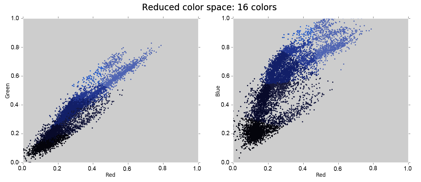
4. We can plot the data again, but this time, we will use new_colors to color the data points accordingly:

In [12]: plot_pixels(img_data, colors=new_colors, 
...      title="Reduce color space: 16 colors")                                           

The result is the recoloring of the original pixels, where each pixel is assigned the color of its closest cluster center:

5. To observe the effect of recoloring, we have to plot new_colors as an image. We flattened the earlier image to get from the image to the data matrix. To get back to the image now, we need to do the inverse, which is reshape new_colors according to the shape of the Lena image:

In [13]: lena_recolored = new_colors.reshape(lena.shape)

6. Then, we can visualize the recolored Lena image like any other image:

In [14]: plt.figure(figsize=(10, 6))
...      plt.imshow(cv2.cvtColor(lena_recolored, cv2.COLOR_BGR2RGB));
...      plt.title('16-color image')

The result looks like this:

It's pretty awesome, right?

Overall, the preceding screenshot is quite clearly recognizable although some details are arguably lost. Given that you compressed the image by a factor of around 1 million, this is pretty remarkable.

You can repeat this procedure for any desired number of colors.

Another potential application of k-means is something you might not expect: using it for image classification.