6.1.1Motivation and scope

In the field of image processing a lot of developments have taken place recently, where image fusion is playing a vital role in research on night vision, military applications and others. Many imaging devices suffer from a limited depth of field, so there is a need for the development of better-quality fused images in multifocus image fusion, as suggested by S. Wei and W. Ke [2]. The works related to image fusion algorithms indicate that all existing algorithms degrade the brightness of fused images and are time consuming. Since image features differ from each other, we need a fusion method based on multiscale decomposition so that all the information in decomposed images can be acquired and fused.

In this chapter, an integrated image fusion method is developed and implemented. Image fusion using PCNN and PCA in a compressive sensing approach, where PCNN and PCA methods are used for fusing low-pass frequency and high-pass frequency component respectively. The performance measures from an experimental result improves of evaluation and visual effect metrics. It has been compared with the other conventional methods based on the frequency components of the image. The fusion results obtained using the proposed methods show a significant improvement in image quality visually and in terms of the evaluation metrics, since the fusion process is done based on the different properties on high pass and low pass frequency components of image.

6.1.2Literature survey

To date, many image fusion methods have been developed that vary in complexity and applications. The main objective of some of the popular image fusion techniques will be discussed in this section.

C. Polh and J. Van Genderen [3] discussed image fusion using PCA (PCA). PCA is used to extract the weighted feature points in image fusion. The principal components of the images are the eigenvectors corresponding to the largest eigenvalues of the co-variance matrix formed by the images. Hence, it reduces redundancy in the fused image data.

H. Yin et al. [4] presented an image fusion technique based on a sparse sampling method or CS. The execution rate is reduced by increasing the quality of the resultant image fused by the integration of non-zero coefficients present in the image. Many errors occur in the conventional approach, such as reconstruction errors, poor fidelity and blocking artefacts that produce uncertain results. To overcome these problems, another fusion-based approach was proposed that includes non-subsampled contourlet transform, which is widely used in decomposition techniques. The CS-based fusion approach can greatly reduce processing speed and guarantee the quality of fused images by integrating fewer non-zero coefficients. Due to the limitations in the conventional CS-based fusion approach, directly fusing sensing measurements may produce results that have greater uncertainty with a high rate of reconstruction errors, and using a single fusion rule may result in problems of blocking artefacts and poor fidelity. An image fusion approach based on CS was developed to solve these problems. The NSCT has been used for image decomposition. A dual-layer PCNN model was used to carry out low-pass sub-band fusion, while high-pass sub-band fusion was used to implement the edge-based fusion rule. For the reconstruction of fused images, a CS matching pursuit algorithm (CoSaMP) was propsed by D. Needell and J. A. Tropp [5].

The motivation behind using PCNN, used to transfer the spatial frequency domain using NSCT for an image fusion procedure, is discussed in Q. Xiao-Bo [6]. Non-subsampled contourlet transform (NSCT) provides flexible multiresolution, anisotropic and directional expansion of images. Compared with the original contourlet transform, it is shift-invariant and can overcome the pseudo-Gibbs phenomenon around singularities. The PCNN is a visual cortex-inspired neural network characterized by the global coupling pulse synchronization of neurons. It has proven suitable for image processing and successfully used in image fusion. Q. Xiao-Bo et al. [6] have shown through experimentation that NSCT is associated with PCNN and can be used in image fusion to make full use of image characteristics. Spatial frequency in the NSCT domain is used to motivate PCNN, and coefficients in the NSCT domain with large firing times are selected as coefficients of fused images. The results obtained from experiments show that the algorithm has performed well using contourlet-based PCNN and wavelet-based PCNN in terms of visual quality and performance metrics.

Yunxiang Tian and Xiaolin Tian [7] have proposed to extend the work of [6]. This includes the intensity hue saturation (IHS) space component from multispectral (MS) images, then decomposition into an I component using NSCT. This method reduces computation time and complexity. Yang Chen and Zheng Qin [8] have presented PCNN-based image fusion in a compression domain approach. In this experiment, the researchers validated the performance measure for three different fusion applications. This produced results in both qualitative and quantitative analysis carried out by Vaibhav R. Pandit and R. J. Bhiwani [9] for applications in image fusion. It has been compared with various conventional image fusion techniques. Hongguang Li et al. [10] have proposed a novel method for image registration and image fusion that has been integrated with cameras in both visible and infrared light on unmanned aerial vehicles (UAVs). This system is very efficient and uses a particle swarm optimization (PSO) hybrid with PCNN and NSCT. Thus, it can be applied to medium-or high-altitude UAVs. Yong Yang et al. [11] have presented two major issues related to multifocus image fusion using fast discrete curvelet transform (FDCT) texture selection and block effects. Experimental results show a reduction in computational complexity and improvement in performance metrics, which has been compared with various state-of-the-art frequency-based fusion and spatial-based fusion methods. B. Rajalingam and R. Priya [12] have implemented, using PCA-DWT, a technique to improve medical image fusion. It is superior to other existing techniques in terms of image quality, visual perception and computational time. Biswas et al. [13] proposed an idea for remote sensing image fusion based on shearlet transform (ST) and PCNN. It can be used to vary the decomposition level of source information in order to maintain geometrical and spectral information. Jun Li et al. [14] discussed image fusion methods applied to infrared and visible images using robust PCA (RPCA) and CS. It preserves background information from infrared and visible images. It computes in parallel in less computation time.

6.2.1Principal component analysis theory

The aim of PCA is to convert a set of observations of correlated variables into a set of values that are linearly uncorrelated variables in a systematic process called principal components. Consider X represents an m-dimensional random vector, where V represents an orthonormal projection matrix such that Y = VTX. The covariance of Y is cov(Y), which is a diagonal matrix, and V−1 = VT:

Multiplying both sides of Equation (6.1) by V we get

V can be written V = [V1, V2, . . .Vd] and

Substituting Equation (6.2) into Equation (6.3)

which can be written

where i = 1, 2. . .d, and Vi is an eigenvector of cov(X).

6.2.1.1PCA image fusion algorithm

Step 1:	First we will generate a two-column matrix A of dimension 2 × N using the two source images and calculate the empirical mean vector along each column Me of dimension 1 × 2.
Step 2:	Subtract M e from each column of A; the resulting matrix X will be of dimension 2 × N.
Step 3:	Find the covariance matrix C of X and calculate the eigenvectors V and eigenvalue D of C and arrange them in decreasing order of their eigenvalues.

Step 4: Calculate the normalized principal components P1 and P2 as follows:

$P_1=\frac{V_1}{\Sigma V}\mathrm{and}{P}_2=\frac{V_2}{\Sigma V}.\left(6.6\right)$

Step 5: The fused image is

$I_{\text{fuse}}\left(x,y\right)=P_1{I}_1\left(x,y\right)+P_2{I}_2\left(x,y\right).\left(6.7\right)$

6.2.2Spatial or simple averaging

The average value of the input image is taken pixel by pixel using a simple image fusion method. The averaging-based fusion rule is as follows:

where IF is the fused image and IA, IB are source components of the image. Each image has three basic multispectral bands of R, G and B.

The relative averaging of two groups, C X and C Y, whichproduced C F, has a single band for all individual pixels, represented in Equation (6.9):

where (m, n) the denotes pixel and spatial domain and i denotes the R, G, B of an image.

6.2.3Image fusion–based wavelet transform

6.2.3.1Discrete wavelet transform

Signals can be represented with higher efficiency using wavelet transforms, which is one of the popular existing techniques. A signal is transformed into a set of basis functions, referred to as a wavelet. The wavelet is chosen and the level of decomposition is chosen at the initial stage. A threshold value is determined after the decomposition of the input data. After applying DWT, the size of the resultant output data vector is the same as that of the applied input data vector. Filters are used to reconstruct the original data. The filtered data are compared to DWT, the continuously transformed data are returned that were larger than the input data vector. The wavelet transform is a well-known signal processing technique that can be used to represent signals with high efficiency. The wavelet transform changes signals into a set of basis functions. These basis functions are called wavelets. A waveform of finite duration having an average value of zero is called a wavelet. A multiscale representation of a signal is given by a DWT. Most applications are not directly associated with scaling factors or wavelet coefficients. A filter band coefficient filters input signals using high-pass and low-pass filters. Let the low pass be h(n) and high pass be g(n). Many sets of filters satisfy the perfect reconstruction conditions, which are approximately symmetric. To use a two-dimensional transform image for analysis, synthesis filter bands can be implemented. In the 2D case, a 1D analysis filter band is initially connected to a segment of the image and then connected to the rows. Let the image representation have N1 rows and N 2 columns; then, after applying the 1D analysis filter band to each column, we have two subband images, each with N1/2 rows and N 2 columns; after applying the 1D analysis filter band to each row of both subband images, we have four subband images, each having N1/2 rows and N 2/2 columns. This is illustrated in Figure 6.3, which shows the output of the DWT of the image and its analysis block.

6.2.3.2Dual-tree complex wavelet transform

Selesnick et al. [15] have shown how DTCWT is a more advanced form of wavelet transform compared to DWT. There are two major advantages of DTCWT over DWT, shift invariant and selective directional into higher dimensions. The major shortcomings in DWT are as follows.

1. Wavelet coefficients tend to oscillate between positive and negative around singularities because of the wavelet bandpass function.
2. A small shift in a signal perturbs the wavelet coefficient oscillation pattern around singularities.
3. The lack of directional selectivity greatly complicates the modelling and processing of geometric image features.

One of the advantages of the DTCWT is that it can be used to implement 2D wavelet transforms, which are more selective with respect to the orientations than in separable 2D DWTs. There are two types of 2D DTCWT: the real 2D DTCWT tree is twice as expensive, while the complex 2D dual-tree DWT is four times as expensive. Both types of complex wavelet transforms have wavelets that are oriented in six distinct directions. Six wavelets are spread in distinct directions. Each subband of the 2D dual-tree transform indicates a specific orientation. A complex 2D dual tree is implemented as four critically sampled and separable 2D DWTs operating in parallel. However, different filter sets are used in the rows and columns. As in real cases, the sum and difference of subband images are determined to obtain the oriented wavelets. A real 2D dual-tree transform of an image is implemented using two critically sampled and separable DWTs operating in parallel. The sum and difference for each subband are taken into consideration. As shown in Figure 6.4, a complex 2D DTCWT is implemented as four critically sampled and separable 2D DWTs operating in parallel. The pair of conjugate filters applied to image decomposition can be expressed as

$\left(H_x+j{G}_x\right)\left(H_y+j{G}_y\right)=\left(H_x{H}_y-G_x{G}_y\right)+j\left(H_x{G}_y+G_x{H}_y\right).\left(6.10\right)$

The complex conjugate of the wavelet transform has positive and negative coefficients of subbands. All corner-to-corner subbands are partitioned in both vertical and horizontal scale of six subbands in the block.

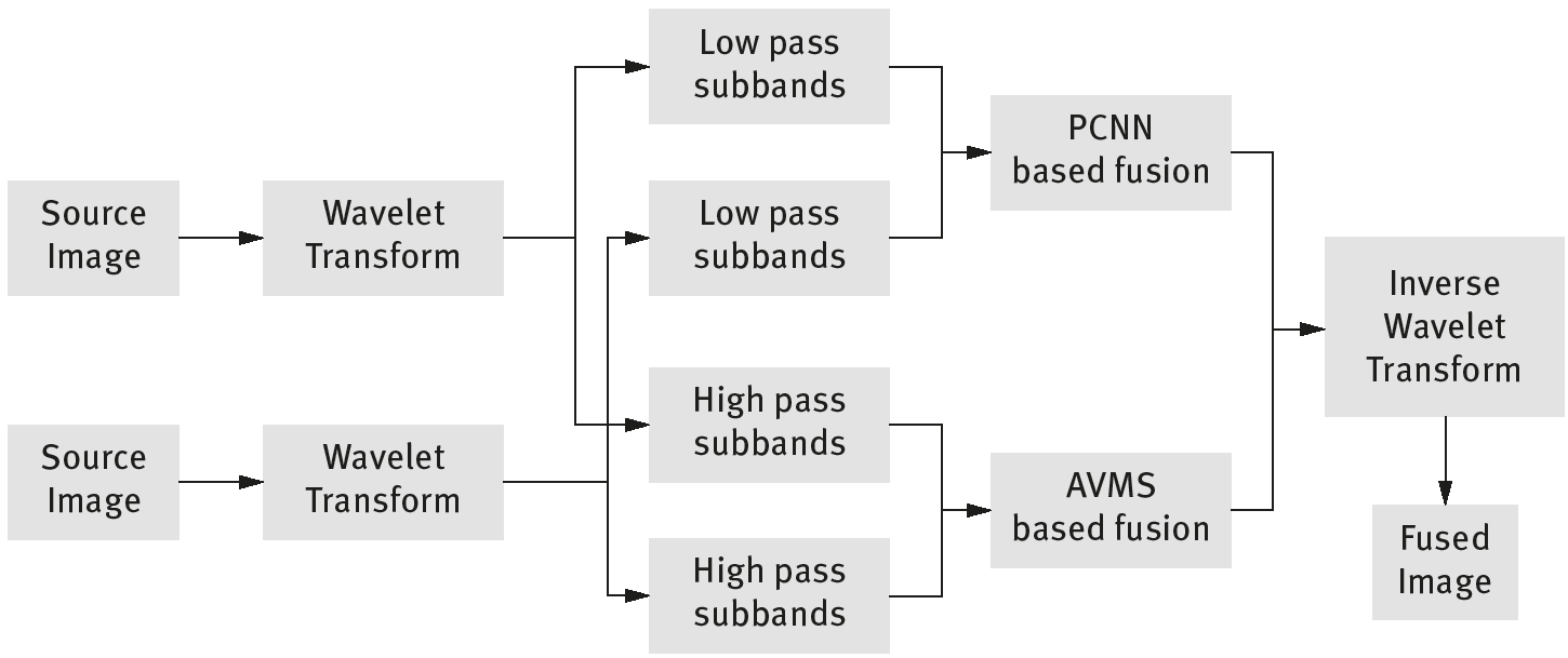
Figure 6.5 shows a general block diagram of a wavelet transform–based image fusion method. It consists of low-pass and high-pass subbands for the fusion process in terms of averaging-based and average mean square–based fusion techniques. The fused images must be obtained by taking the inverse wavelet transform from the previous step.

6.2.4Pulse-coupled neural network

This works on the principle of optic nerves, which transmit data observed by the eyes to the brain and the visual cortex. Generally, the input data are then transferred to fiber pathways and finally processed. The most predominant factor of the visual cortical area in the visual cortex is visual processing, and nearly all visual signals reach the cortex via the primary visual cortex. Eckhorn et al. [16] in the late 1980s discovered that binary images are created in an oscillating manner by the mid-brain, which can extract different features from the visual impression when they have to read the cat visual cortex [16] An actual image is then created in the cat’s brain by the help of these binary images. Inspired by this biological system, machines are also trained to perform the functions of the human brain. This leads to the new structure of a neural network model, called Eckhorn’s model, to simulate the behaviour of the visual cortex. From the case study report on the linking field model H. Ranganath et al. [17] discussed PCNN based on the Eckhorn model with some modifications.

Figure 6.6 shows a PCNN model that consists of two major components: feeding and linking. The link between neighbourhood neurons is established by the symmetric weights M and W. The input stimulus S is given to the feeding compartment. The PCNN model and its components are determined by 6.11

where ∗ represents the convolution operator, ‘n’ represents the number of iterations, ‘Y’ represents the output of neurons from (n − 1) iterations. The compartments have a memory of their previous state, which decays over time by the exponent term. The constants VF and VL are normalizing constants. After receiving the inputs the feeding and linking compartments are combined together to generate the internal state of the neurons. The internal activity U is expressed as in Equation (6.13), where β is the controlling parameter:

Thus, the internal activity of neuron U has various states mapped with the dynamic threshold, θ, to produce output to another neuron ‘Y’ as given in Equations (6.14) and (6.15):

If (U > θ), then the neuron fires very high to the threshold value of Y and converges until a neuron gets fired. The dynamic activity of the threshold property is given in Equation (6.16),

where Vθ is a constant with a significantly larger value than the average value U and order of magnitude. Initially, values of F, L, U and Y are all set to zero. The values of the θ elements are initially 0 or some larger value depending upon the application. From this activity, in both the feeding and linking compartments, the neuron receives some source stimulus S and stimulus from the neighbourhood state. The pulsing nature of the PCNN can be observed by looking at the rise and fall of the threshold value with the corresponding rise and fall of the internal activity value.

6.2.4.1General image fusion algorithm based on PCNN

A data flow diagram of the PCNN algorithm is shown in Figure 6.7 and follow the steps given below,

Step 1:	Segment input data into subbands of low pass and high pass and are called source data.
Step 2:	The focus measure for the low-pass subband is given as an input to the PCNN to activate the neural activity using spatial focusing.
Step 3:	Calculate the firing times Tij using the following equations:

$F_{ij}\left[n\right]=S_{ij},\left(6.17\right)$

$L_{ij}\left[n\right]=e^{\alpha l}{L}_{ij}\left[n-1\right]+V_L\left(WXY\right),\left(6.18\right)$

$U_{ij}\left[n\right]=F_{ij}\left[n\right]\left(1+\beta L_{ij}\left[n\right]\right),\left(6.19\right)$

${\theta }_{ij}\left[n\right]=e_{ij}^{\alpha }\left[n-1\right]+V{Y}_{ij}\left[n\right],\left(6.20\right)$

$Y_{ij}\left[n\right]=1;\text{if}{U}_{ij}\left[n\right]>{\theta }_{ij}\left[n\right],\left(6.21\right)$

$Y_{ij}\left[n\right]=0;\text{Otherwise}\text{,}\left(6.22\right)$

$T_{ij}=T_{ij}\left[n-1\right]+Y_{ij}\left[n\right].\left(6.23\right)$

We can take the parameters as

$\begin{array}{lll}\alpha L=0.06931,\hfill & \alpha \theta =0.2,\hfill & \beta =0.2,\hfill \\ V_L=1,\hfill & V=20,\hfill & W=\left[\begin{array}{ccc}0.707& 1& 0.707\\ 1& 0& 1\\ 0.707& 0& 0.707\end{array}\right]\hfill \end{array}$

and the iteration is n = 200.

Step 4: Obtain the decision map D F,ij and select the coefficients xF,ij which means that the coefficients with large firing times (large T values) are selected as coefficients of the fused image, since the value of each pixel in the firing map images is equal to the firing times, and a longer firing time corresponds to more information, based on the following equations:

$D_{F,ij}\left[n\right]=1;\text{if}{T}_{1,ij}\left[n\right]\ge T_{2,ij}\left[n\right],\left(6.24\right)$

$D_{F,ij}\left[n\right]=0;\text{if}{T}_{1,ij}\left[n\right]<T_{2,ij}\left[n\right],\left(6.25\right)$

$X_{F,ij}=x_{1,ij}\left[n\right];D_{ij}\left[n\right]=1,\left(6.26\right)$