3.1Introduction

The world has become an automated one as we move closer towards white collar automation faster than ever before. One critical insight that only people can provide are visual abilities that help them to manoeuvre in real life and provide value to society. Deep learning is playing catch-up in this part of image and vision processing with newer algorithms and better performance aspects. This chapter provides a detailed review of the topic using a sequential time line of advances in the image and video processing power of today’s algorithms with a final note on the growing use of parallel computing hardware, which is being used for training these deep neural networks.

The chapter introduces the concept of neural networks and how such networks can be used for training on a variety of different types of data to represent all kinds of policies. It then covers image and video processing techniques like enhancement, upsampling, super resolution and quality assessment of images and how they have advanced in their respective techniques along with how parallel computing and deep learning fit together.

Deep learning is a relatively new field what began with the advent of greater computing power, but the term started to be used in the research community around 1986 when Dechter et al. [1] published a paper introducing a pseudo-deep learning concept to solve constraint specification problems, a niche application for solving constraint specification problems. The approach looks at backtracking search that was used in Prolog for solving dead-end situations and proving truth maintenance system theorem. The researchers showed that it was possible to use backtracking and back-propagation for learning methodology in neural networks [2]. The first official work on learning algorithms was published by Aizenberg et al. in their book [3].

Deep learning uses a layered structure of neurons that take a large data set, propagate the data forwards and backpropagate the results using a loss function and gradient over the connections between the layers, which simulates the learning process [4]. Deep learning has been extremely successful in image classification work with the advent of convolutional neural networks (CNNs) [5]. This architecture involves using a convolutional layer for feature extraction along with maxpooling and fully connected layers for classification.

3.2Image and video enhancement

Image enhancement generally includes techniques that are used to modify an image or a video in such a way that its quality and visibility increase. This can be done in a number of traditional ways that can be broadly split into two categories: spatial domain and frequency domain.

Spatial domain methods alter an image by directly altering the pixel values in the image using transformations and filters. This direct change allows for less complex yet less sophisticated changes to be made to the image. Frequency domain methods first convert an image from one domain to another domain and then transform the image using various techniques before converting the image to the original domain [6].

Deep learning methods for image enhancement usually apply generative models to use previously learned features and apply them to a noisy image to generate a more aesthetically pleasing image that has enhanced features [7]. Another method involves using a bilateral architecture to take the low-resolution and high-resolution versions of the same image and use a CNN on the low-resolution image to generate coefficients that are later added to the high-resolution version [8].

3.2.1Pixel processing operations

To conduct operations in the spatial domain, the earliest applications begins in the neighbourhood of the pixels themselves. Because each pixel in an image is surrounded by other pixels, they are subjected to a series of transformations. These transformations themselves enhance the image, but their most popular use is to act as a preprocessing method to assist in making further, complex changes. Some transformations include thresholding transformations, power-law transformations and logarithmic transformations. Specifically for image enhancement, various classes of neural filters have been proposed. A neural filter primarily requires processing an image through two separate classes of a decision-based filter. The output is then passed on to a feedforward neural network.

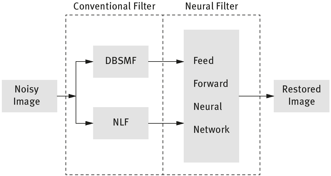
The Figure 3.1 displays two filters, a conventional filter and a neural filter. Both together act as an impulse noise removal filter. Initially the noisy image is given to conventional filters like a non-linear filter(NF) and descision based switching median filter (DBSMF). It is then processed further using a simple feedforward neural network (Figure 3.2). The fine edges are preserved and noise is eliminated using a backpropagation algorithm.

3.2.2Histogram-based image enhancement

These are contrast enhancement techniques, and every technique is dependent upon a histogram of the image. To perform any operation in the frequency domain, there has to be a representation of the tonal distribution of the image. Hence, after pixel level transformations are undertaken, a computational model is implemented to automatically enhance the image following the learned style.

Learning image enhancements based on its visual style is a challenging task; it is a highly observational and visceral process that deals with the information embedded in an image based upon its pixel colours and their frequency. To learn an enhancement style, a quantitative relationship needs to be established.

Deep neural networks are implemented to generate a mathematical model based upon quantitative relationships. Zicheng Yang et al. [9] elaborated upon one such deep neural network; the principal purpose of the network was to generate an intrinsic colour mapping function that maps each pixel’s colour in a noisy to enhanced image. The architecture is elaborated upon in the following figure.

In Figure 3.3, the neurons above the dotted line define how the intrinsic function is computed. The weights between the yellow and blue neurons are all components of the quadratic colour basis, and the identity function is the activation function within the purple and yellow neurons.

This architecture is superior to its predecessors as it is able to learn complex and highly non-linear photo enhancement styles. It is capable of enhancing preferred contextual features using the robust regression capability of deep neural networks.

3.3Image super resolution

Another scenario of image enhancement can also be in image super resolution, where low-resolution images are taken and bumped up to create a higher-resolution version of the same image. This use case has been distinguished from image enhancement as research in this category has been extensive regarding generative models and is beyond the scope of this chapter (Figure 3.4).

Historically, methods like maximum likelihood, maximum a posteriori, joint map restoration and Bayesian treatments have been used for super resolution, which involves directly altering the pixels of an image to produce a better image. These methods can also be categorized as spatial domain methods for image enhancement [10].

Generative models find their application here as well by taking the original image and increasing their resolution by simultaneously training two networks that use game theory to adversarially train themselves and produce true-to-life images [7].

3.4Image upsampling

Image upsampling refers to the task of enlarging an image with an integral value such that the image can fit the new dimensions. Image upsampling usually replicates rows and columns according to the needs of the dimension being scaled to. Deep learning allows an image to be upsampled with better quality along with higher dimensions as well. Image upsampling is the linear opposite of image downsampling, where the image data are reduced to fit the new resolution. Hence, images can be upsampled by either adding new information to them or by using the existing information to produce a larger version of the same image.

Deep learning can be used in this domain of image processing as many algorithms can be used to generate new images from previously known image data sets. This allows neural-network-based models to produce upsampled images from a data set whose images need to be upsampled. Since the algorithm can provide much more accurate upsampled data, this section discusses the various deep learning methodologies that can produce comparable and even better results than previously known techniques.

Traditional image upsampling techniques involve Fourier upsampling, which uses Fourier transformations to produce upsampled images by adding pixel data for the missing values by transforming the k-nearest neighbours (k-NN) of a pixel through a Fourier transform and adding those values. This method usually involves a 4× Fourier transform with reconstruction or alias [13].

A tried and tested deep learning algorithm involves yet again generative adversarial networks called Laplacian Pyramid Generative Adversarial Networks [14] that use a Laplcaian Pyramid to create missing pixel values and uses adversarial training on a generator and a discriminator to form the pyramid itself.

3.4.1Upsampling using neural networks

Deep neural networks are also used in image upsampling. The deep learning method used is known as a deep network cascade [15]. The upscaling is gradual, layer by layer with the introduction of a scaling factor. It eventually attains the higher resolution required. The small refinements are based on searching for non-local self similarities in order to improve the higher-frequency details of the segments to which the image is partitioned. The segments are then absorbed into each layer of the cascading multistack network of a local auto-encoder for noise suppression and to enhance the coherence among the overlapping patches enhanced by the aforementioned procedure (Figure 3.6).

3.5Image and video quality assessment

Image quality assessment is a way to assess how good an image is in comparison to either a reference image or a general set of parameters. These parameters can be resolution, contrast, saturation levels, colour accuracy and or other metrics. Image quality assessment is a necessary component of any image processing system as it makes it possible to compare how the processing application is working.

Traditionally, image quality assessment was done using the visibility of errors (differences) between a distorted image and a reference image using a variety of known properties of the human visual system [16]. Another method used for such quality assessment is called a structural similarity index that extracts the base structure of an image by eliminating the overlying luminance and contrast features and satisfies a few conditions to provide an image that is structurally similar to the original one [17].

More recent deep learning approaches to quality assessment use a CNN to learn patch features in the spatial domain that are used to determine the quality of an image without any reference images for a base comparison [18].

3.5.1Error sensitivity–based method

According to Wang et al. [19], image quality measurement is used for three primary reasons: to monitor quality for quality systems, to benchmark various algorithms that generate or modify images, and to optimize the image generation process of algorithms or techniques.

One image quality assessment technique that is used is the error sensitivity method that uses a full-reference model to compare images and calculate the error between images. First, two images are subjected to different preprocessing techniques, which then decompose them into difference channels. The error for each channel, weighted by a contrast sensitivity function (CSF), is then transferred to an error-masking function, which then sums the error using a summation function, which tells us the quality or the distortion measurement of the image. This summation function can also use a Minkowski error-pooling function. This method has certain drawbacks due to the following assumptions, mainly:

–The reference image is a perfect image

–The visual channels in the images can be simulated by channel transformations

–In each channel, the interactions between coefficients is small enough to be ignored

–The image quality perceived is done by the early vision system

–Active visual processes, such as change of fixation point, are ineffective

3.6Parallel computing techniques

Parallel computing refers to a computing paradigm that uses multiple simultaneously processed threads that can be used for varied applications such as graphic processing, neural network training and hyperthreading. This new methodology has been become famous due to its application in research, with the most common form of hardware used in such systems being multicore processors and graphics processing units. This work relies heavily on the latter for network training. It also looks at the various motivations, shifts and tensions that have surrounded the use of multiple cores instead of one for macro and niche processing in various fields of study [20].

The image processing problems that require vast amounts of time for processing or handling large amounts of data can be addressed with parallel computing techniques. The principal idea involves dividing a problem into simple tasks and solving them concurrently. The best case scenario is attained when the total time can be divided among the total tasks. Not all problems can be solved by parallel image processing, and not all methodologies require coding in a parallel form. Every parallel coded technique has features of an efficiency or a correcting operation. These features mainly include granularity, synchronization, latency, scalability and a defined type of parallel processing.

Granularity determines the number of key units in a frame; it is represented by two types, coarse grained and fine grained. Coarse grained is indexed to having few tasks but each with intensive computing methods, whereas fine grained is indexed to having a large number of small tasks with no specific intensive task, so with less intensive computing.

Synchronization is embedded to ensure that no two processes overlap. Latency is defined as the time of transition of information from request to declaration. Scalability is the metric that indicates the ability of an algorithm to maintain its efficiency by increasing the number of processors in proportion to the size of a problem.

3.6.1Data parallelism

The objective of any learning algorithm is to minimize the loss function in a methodical manner. In the case of deep neural networks, there is a loss function introduced that is an independent and differential function of the model hyper-parameters. In the case of parallel image processing, methods are generated to iteratively update the parameters with the aim of reducing the net-loss function. One way to do this is to perform mini-batch gradient descent, but it is computationally expensive and time consuming. Hence the weight update procedure needs to be parallelized to achieve accelerated learning.

Data parallelism is a procedure to distribute computing among different machines in a way that computation is performed locally on each machine using the complete model but only for part of the full data set. A representation of data parallelism for updating parameters is demonstrated in Figure 3.9. The most commonly used version of data parallelism is the implementation of parallel stochastic gradient descent (ParallelSGD) [21]. This acts as a substitute for a multibatch stochastic gradient descent algorithm.

Once every machine has the data required to go over the distribution of the whole data set, ParallelSGD is run on each machine locally. The communication time and communication cost are the factors that additionally contribute to the net error. Upon updating the parameters, a global communication procedure is performed to send the information to the driver machine, where it will be further be analysed independently. BitTorrent aggregate communication is the protocol that has achieved the best result thus far.

3.7Modern deep neural architectures

The most widely used application of image processing techniques is in the implementation of deep neural networks. In the contemporary world, almost all types of computational processing can be optimized by the implementation of deep neural architectures [22].

Deep learning techniques were initially applied for adapting to parallel strategies for time series learning [23]. Along time, the computational load for time series learning was multithreaded. Deep neural networks have been applied to several classification and recognition problems on images [24]. Part of its success is due to the automatic feature extraction at different levels of abstraction [25]. In the past decade, there have been multiple designs and heuristics to implement learning in deep neural networks for images. Those that are trending and heavily discussed in the community include deep CNNs (DCGANs) [26], adversarial learning [27], deep residual learning [28] and shallow learning algorithms [29]. We would like to elaborate on the neural architectures created to tackle the different tasks in the chain of image processing. The following subsections discuss the degrees of success attained by deep neural networks in each task for which they have been used.

3.7.1Image preprocessing

Preprocessing entails any operation performed upon an input-actuated image, with the output being a full image. It is the first step in an image processing chain, following image acquisition. The operations performed during preprocessing can be broadly classified into three categories: image reconstruction, image restoration and image enhancement. Reconstruction consists in building up the image based upon the actuated measurements. Restoration entails the removal of any aberrations that are introduced by the sensor, for instance noise. Enhancement deals with the improvement of certain accentuated features.

3.7.1.1Image restoration

Neural networks are widely used in image restoration due to their functionality of excellently adapting to the local nature of a problem. They can be implemented for various use cases, usually alternating between restoration and learning cycles. Contemporary neural network processing methods have led to the creation of efficient very-large-scale integration architectures for image restoration, mainly due to their high parallel image processing features.

Dianhui Wang et al. [30] introduced a pattern-learning-based image restoration network for highly deteriorated images. The regularization function that was used to recover the artefacts uses the edge information obtained from the source images. Image similarity was the criterion used by this network to attain, though the judgment is subjective, a quality enhancement. This paper established a mathematical foundation for the use of modern neural networks to perform the task of preserving edge information.

Deng Zhang et al. [31] introduced a neural network designed to eliminate pulse noise. The method was closely based upon anisotropic diffusion methods. The network was termed a pulse-coupled neural network (PCNN) and implemented a denoising method using convolution. The researchers further compared their performance to the traditional filters such as median, Weiner filter, Lee filter and anisotropic diffusion filter. This paper established the benchmark in noise suppression along with edge detail preservation.

3.7.1.2Image reconstruction

Using knowledge from the degrading factors and building up the original image is defined as image reconstruction. Contemporary image restoration techniques have one common deficiency, poor convergence properties. The local minima that the heuristics converge upon are speculative for real imaging applications. The key problem is the recovery of the information of the lost details in the present blurred image. Multilayer Feedforward Neural Network Based on Multi-Valued Neurons (MLMVN), CNN and backpropagation neural network (BPNN) are used to attain high-quality restored images by fast neural computation. They are commonly used because they do not employ lengthy training algorithms.

As a recent trend, Suhasini et al. [32] showcases the use of a BPNN for blur parameter identification. The BPN is trained upon the parameters extracted from a degraded image and the network is simulated to restore the image. It employs deblurring with convolution with a Lucy Richardson algorithm. Backpropagation neural networks have displayed great success in areas requiring high computation rates.

3.7.1.3Image enhancement

Image enhancement involves sharpening image features like boundaries, contrast and edges. There is no increment in inherent information content in the image data. The dynamic range of these features is increased so they can be more easily visually detected. The prime objectives are noise reduction, removal of inhomogeneities in the background and feature extraction.

Entezarmahdi et al. [33] set the benchmark in neural image enhancement methods compared to stationary methods. This paper defines two transform-based super resolution methods for image enhancement. As per the first method, the wavelet transform coefficients of the lower-resolution image is used as data to train a neural network. In the second method, a contourlet transform replaces the wavelet transform. The results of this experiment demonstrated superiority in performance to its predecessors.

3.7.2Data reduction

The best-known applications in data reduction are feature extraction and image compression. All image compression algorithms involve encoding and decoding, and for these steps a neural network is designed.

3.7.2.1Image compression

There are two widely observed compression techniques based on modular approaches and on neural networks. The major advantages of using an artificial neural network (ANN) is that the model is adaptable, so when trained on any particular image data set, it gives significantly better compression rates.

Jin Wang et al. [34] use a custom-designed neural network based upon wavelet transforms. Their use case was ECG data compression, but their novel approach is to continuously adjust the initial weights while accelerating the convergence speed. They compare the performance of their network to a wavelet compression algorithm, their results were more satisfactory compared to BPNN and principal component analysis (PCA) methods.

3.7.2.2Feature extraction

Feature extraction can be seen as a special form of data reduction in which the aim is to find the subset of variables that are informative based on the image data. It is crucial to make a distinction between the involvement of supervised and unsupervised ANNs for feature extraction. Both learning methods have established significant benchmarks in feature extraction compared to traditional techniques such as PCA.

Wu Jiang et al. [35] have developed a novel algorithm for image-based feature extraction built upon the PCNN mentioned earlier. Execution time and size are the parameters used to evaluate the results. The experimental results proved that they outperformed traditional Euclidean algorithms.

3.7.3Image segmentation

Generating salient regions by clustering pixels is the aim of image segmentation. Most neural approaches apply segmentation directly to pixel data, whereas others approach it by generating patterns at the feature level. Hence the two approaches can be simplified to clustering and pattern recognition.

3.7.3.1Clustering

All images contain well-formed information that can be inferred by humans upon viewing the images. When approaching learning methods in an unsupervised method and dealing with the congregation of unlabeled data, the process of clustering may be considered. Clustering basically involves determining the spatial thresholds that reveal the similarity and dissimilarity of certain objects in connection with others.

Li Jing et al. [36] propose a method based upon general regression neural network (GRNN) and fuzzy c-means (FCM) clustering algorithms. Their method involves the creation of pattern neurons to embed and extract identified locations based upon the embedding strength on the human visual system (HVS). PSNR (Peak Signal to Noise Ratio) and BCR (Bit Correction Rate) were used to evaluate the performance of their method.

3.7.3.2Pattern recognition

The perceptive powers of the human mind allows us, over time, to recognize trained objects. Pattern recognition is defined as action based upon the category of pattern identification. An ANN is an impressive tool for classification and pattern-recognition tasks.

Budiwati et al. [37] describe one of the most popular neural networks, which was designed for Japanese character recognition and based upon a BPNN. There are multiple writing systems in the Japanese language, and there was a need for pattern recognition to distinguish the writing styles of Kanji and Kana. The performance of the neural network was compared to the computational receiver operating characteristic (ROC). It set a benchmark in pattern recognition as it attained an accuracy of 92.29% from 3,956 images to train upon.

3.7.5Image understanding

Image understanding is the most problematic area of image processing. It entails building correlations with the content of an image using techniques such as segmentation and recognition. It involves two major steps, scene analysis and object arrangement.

3.7.5.1Scene analysis

Scene analysis is quite different in comparison to the recognition of different objects. It involves inherent changes in variation, illumination and noise. Neural networks act as classifiers by generating multiple weighted connections.

Seiji et al. [40] set a benchmark in image searching by introducing a novel architecture, a sandglass-type neural network. It was built for the use case of browsing searches and similarity-based image retrieval. The authors use the maxi-min distance algorithm (MDA) for image preprocessing.

3.7.5.2Object arrangement

Any fragment of an image that could be categorically recognized as a single unit is referred to as an object. The most popular problem statement tackled using object arrangement is that of real time object tracking. Neural networks are most commonly used for tracking and arrangement purposes because of their capability of non-linear mapping among varied complexities.

Hiremath and Kodge [41] have established modern benchmarks in locating object boundaries using active contours. They employ a k-NN along with neural classifiers. The performance criteria of MSE (Mean Square Error) and SD (Standard Deviation) is used for sampling and distribution of these features.

3.7.6Image optimization

Image optimization deals with the selective process of choosing the best element from a given set of elements based upon some deciding criteria. Optimization problems include a wide variety of functions, each one catering to a specific domain. The most common image optimization technique is graph matching.

3.7.6.1Graph matching

Labelling the significant objects in an image by identifying them is defined as image interpretation. Image interpretation conducted across the graphical representation is termed graph matching. The represented graph is further partitioned in accordance with the criteria formulated for segmentation into clusters.

Various neural network architectures are applied subject to a particular graph matching problem. Zinkevich et al. [21] introduced a novel architecture based upon the multilevel perceptron neural network. It was designed for the use case of thumb-print classification, and training is performed by a vanilla ANN. Its performance criterion is the MSE and sets the lowest MSE value at less than 0.1.

3.8Conclusion

This chapter presented an in-depth explanation of various deep learning techniques that are used in various tasks performed along the image processing chain. Huge amounts of neural architectures have been developed by researchers in recent decades, and we provided an explanation regarding techniques implemented for particular tasks in image processing for each model. Case studies have shown that hybrid models demonstrate superior performance in comparison to conventional models. The model that sets the highest benchmark was described briefly, and each task of image processing used in the model was described in detail.

Even though conventional models have high accuracy, newly defined hybrid models are tailored to a particular use case. Combining these conventional models in accordance with their use case yields higher accuracy and contributes to the individual performance of the models. Hence, the highly iterative and learning-based approach of deep learning techniques shows better performance for tasks in image processing.

Bibliography

[1]Dechter R. Learning while searching in constraint-satisfaction-problems. In Kehler T, editor, AAAI, pages 178–185. Morgan Kaufmann, 1986.

[2]Kelley HJ. Gradient theory of optimal flight paths. ARS Journal, 30(10):947–954, 1960.

[3]Igor Aizenberg JPLV Naum N. Aizenberg. Multi-Valued and Universal Binary Neurons. Springer US, 2000.

[4]Hadsell R, Erkan A, Sermanet P, Scoffier M, Muller U, and LeCun Y. Deep belief net learning in a long-range vision system for autonomous off-road driving. In Proc. Intelligent Robots and Systems (IROS’08), 2008.

[5]Krizhevsky A, Sutskever I, and Hinton GE. Imagenet classification with deep convolutional neural networks. In Advances in neural information processing systems, pages 1097–1105, 2012.

[6]Maini R and Aggarwal H. A comprehensive review of image enhancement techniques. CoRR, abs/1003.4053, 2010.

[7]Radford A, Metz L, and Chintala S. Unsupervised representation learning with deep convolutional generative adversarial networks. CoRR, abs/1511.06434, 2015.

[8]Gharbi M, Chen J, Barron JT, Hasinoff SW, and Durand F. Deep bilateral learning for real-time image enhancement. CoRR, abs/1707.02880, 2017.

[9]Yang J, Ren P, Chen D, Wen F, Li H, and Hua G. Neural aggregation network for video face recognition. CoRR, abs/1603.05474, 2016.

[10]Yang J and Huang T. Image super-resolution: Historical overview and future challenges. Super-resolution imaging, pages 20–34, 2010.

[11]Liu P and Fang R. Learning pixel-distribution prior with wider convolution for image denoising. CoRR, abs/1707.09135, 2017.

[12]Figueiredo MAT. Synthesis versus analysis in patch-based image priors. CoRR, abs/1702.06085, 2017.

[13]Shan Q, Li Z, Jia J, and Tang CK. Fast image/video upsampling. ACM Transactions on Graphics (TOG), 27(5):153, 2008.

[14]Denton EL, Chintala S, Fergus R, et al. Deep generative image models using a laplacian pyramid of adversarial networks. In Advances in neural information processing systems, pages 1486–1494, 2015.

[15]Schlemper J, Caballero J, Hajnal JV, Price AN, and Rueckert D. A deep cascade of convolutional neural networks for dynamic MR image reconstruction. CoRR, abs/1704.02422, 2017.

[16]Mannos J and Sakrison D. The effects of a visual fidelity criterion of the encoding of images. IEEE transactions on Information Theory, 20(4):525–536, 1974.

[17]Wang Z, Bovik AC, Sheikh HR, and Simoncelli EP. Image quality assessment: from error visibility to structural similarity. IEEE transactions on image processing, 13(4):600–612, 2004.

[18]Kang L, Ye P, Li Y, and Doermann D. Convolutional neural networks for no-reference image quality assessment. In Proceedings of the IEEE conference on computer vision and pattern recognition, pages 1733–1740, 2014.

[19]Wang Z, Bovik AC, and Lu L. Why is image quality assessment so difficult? In Acoustics, Speech, and Signal Processing (ICASSP), 2002 IEEE International Conference on, volume 4, pages IV–3313. IEEE, 2002.

[20]Asanovic K, Bodik R, Demmel J, Keaveny T, Keutzer K, Kubiatowicz J, Morgan N, Patterson D, Sen K, Wawrzynek J, Wessel D, and Yelick K. A view of the parallel computing landscape. Commun. ACM, 52(10):56–67, October 2009.

[21]Zinkevich M, Weimer M, Li L, and Smola AJ. Parallelized stochastic gradient descent. In Lafferty JD, Williams CKI, Shawe-Taylor J, Zemel RS, and Culotta A, editors, Advances in Neural Information Processing Systems 23, pages 2595–2603. Curran Associates, Inc., 2010.

[22]Blum C, Puchinger J, Raidl GR, and Roli A. Hybrid metaheuristics in combinatorial optimization: A survey. Applied Soft Computing, 11(6):4135 – 4151, 2011.

[23]Coelho IM, Coelho VN, da S. Luz EJ, Ochi LS, Guimarães FG, and Rios E. A gpu deep learning metaheuristic based model for time series forecasting. Applied Energy, 201:412 – 418, 2017.

[24]Sun Y, Chen Y, Wang X, and Tang X. Deep learning face representation by joint identification-verification. In Advances in neural information processing systems, pages 1988–1996, 2014.

[25]Ojha VK, Abraham A, and Snášel V. Metaheuristic design of feedforward neural networks: A review of two decades of research. Engineering Applications of Artificial Intelligence, 60:97 – 116, 2017.

[26]Krizhevsky A, Sutskever I, and Hinton GE. Imagenet classification with deep convolutional neural networks. In Advances in neural information processing systems, pages 1097–1105, 2012.

[27]Lowd D and Meek C. Adversarial learning. In Proceedings of the Eleventh ACM SIGKDD International Conference on Knowledge Discovery in Data Mining, KDD ’05, pages 641–647, New York, NY, USA, 2005. ACM.

[28]He K, Zhang X, Ren S, and Sun J. Deep residual learning for image recognition. In The IEEE Conference on Computer Vision and Pattern Recognition (CVPR), June 2016.

[29]Dechter R. Enhancement schemes for constraint processing: Backjumping, learning, and cutset decomposition. Artificial Intelligence, 41(3):273 – 312, 1990.

[30]Man Z, Lee K, Wang D, Cao Z, and Khoo S. Robust single-hidden layer feedforward network-based pattern classifier. IEEE transactions on neural networks and learning systems, 23(12):1974–1986, 2012.

[31]Zhang D, Mabu S, and Hirasawa K. Image denoising using pulse coupled neural network with an adaptive pareto genetic algorithm. IEEJ Transactions on Electrical and Electronic Engineering, 6(5):474–482, 2011.

[32]Suhasini A, Palanivel S, and Ramalingam V. Multimodel decision support system for psychiatry problem. Expert Systems with Applications, 38(5):4990–4997, 2011.

[33]Entezarmahdi SM and Yazdi M. Stationary image resolution enhancement on the basis of contourlet and wavelet transforms by means of the artificial neural network. In Machine Vision and Image Processing (MVIP), 2010 6th Iranian, pages 1–7. IEEE, 2010.

[34]Wang J, She M, Nahavandi S, and Kouzani A. Human identification from ecg signals via sparse representation of local segments. IEEE Signal Processing Letters, 20(10):937–940, 2013.

[35]Jiang H, Wang J, Yuan Z, Wu Y, Zheng N, and Li S. Salient object detection: A discriminative regional feature integration approach. In Proceedings of the IEEE conference on computer vision and pattern recognition, pages 2083–2090, 2013.

[36]Cliff MA, Dever MC, Hall JW, and Girard B. Development and evaluation of multiple regression models for prediction of sweet cherry liking. Food Research International, 28(6):583–589, 1995.

[37]Budiwati SD, Haryatno J, and Dharma EM. Japanese character (kana) pattern recognition application using neural network. In Electrical Engineering and Informatics (ICEEI), 2011 International Conference on, pages 1–6. IEEE, 2011.

[38]Kim JM and Kang MA. A study of face recognition using the pca and error back-propagation. In Intelligent Human-Machine Systems and Cybernetics (IHMSC), 2010 2nd International Conference on, volume 2, pages 241–244. IEEE, 2010.

[39]Yilmaz A, Javed O, and Shah M. Object tracking: A survey. Acm computing surveys (CSUR), 38(4):13, 2006.

[40]Ito S, Mitsukura Y, Fukumi M, Akamatsu N, and Omatu S. Scene image analysis by using the sandglass-type neural network with a factor analysis, volume 2, pages 994–997. Institute of Electrical and Electronics Engineers Inc., 2003.

[41]Kodge BG and Hiremath PS. Elevation contour analysis and water body extraction for finding water scarcity locations using DEM. CoRR, abs/1404.3002, 2014.