
Chapter 2
Two-point methods
This chapter is devoted to two-point root-finding methods. Traub’s study (Traub, 1964) of two-point methods of third order is the first systematic investigation of multipoint methods. Although these methods are not optimal, in Section 2.1 we give a short review of Traub’s methods for their great influence to the later development of multipoint methods. To demonstrate developing techniques, several different derivations of the Ostrowski method originally proposed in 1960 (the first two-point method of order four) are presented in Section 2.2. Derivation and convergence analysis of two families of optimal two-point methods, proposed by the authors of this book, are presented in Sections 2.3 and 2.4. These families give a variety of fourth-order methods. Aside from the well-known Jarratt methods, in Section 2.6 we present a generalized family of Jarratt’s type that produces many two-point methods of optimal order four. Section 2.7 concerns with optimal two-point methods for finding multiple roots. It is interesting to note that the first two-point methods for multiple roots of optimal order were not constructed until 2009, almost half a century after the first optimal two-point method (Ostrowski, 1960) for finding simple roots.
2.1 Cubically convergent two-point methods
According to Theorem 1.6, any one-point iteration function which depends explicitly on f and its first ![]() derivatives cannot attain higher order than r, that is, the informational efficiency
derivatives cannot attain higher order than r, that is, the informational efficiency ![]() of any one-point method
of any one-point method ![]() cannot exceed 1 even by employing additional derivatives of higher order, where
cannot exceed 1 even by employing additional derivatives of higher order, where ![]() is the number of F.E. per iteration. This was the reason and motivation for developing multipoint or multistep methods (both terms are used in the literature). The full benefit of multipoint methods occurs in their increased efficiency, namely, higher order of convergence is attained with fewer F.E. This is possible only by the reuse of information in every iteration step.
is the number of F.E. per iteration. This was the reason and motivation for developing multipoint or multistep methods (both terms are used in the literature). The full benefit of multipoint methods occurs in their increased efficiency, namely, higher order of convergence is attained with fewer F.E. This is possible only by the reuse of information in every iteration step.
2.1.1 Composite multipoint methods
Composite multipoint methods were extensively described in Traub’s book (Traub, 1964). The first two-point methods, based on Theorem 1.3, are illustrated by the following example.
Example 2.1
Let

According to Theorem 1.3, the iterative method defined by the composition
![]()
has the order ![]() . If
. If ![]() is an initial approximation to the root
is an initial approximation to the root ![]() , Newton-Halley’s composite method can be written as
, Newton-Halley’s composite method can be written as
 (2.1)
(2.1)
We note that this method uses the calculation at two points ![]() and
and ![]() so that it can be referred to as two-point method or two-step method.
so that it can be referred to as two-point method or two-step method.
The computational efficiencies of Newton’s method ![]() , Halley’s method
, Halley’s method ![]() , and the composite two-step method
, and the composite two-step method ![]() are (in view of (1.13))
are (in view of (1.13))
![]()
Notice that Halley’s method possesses the highest efficiency so that the construction of the composite method in this case is not justified. Any construction of composite I.F. should be performed with a tendency to decrease the number of F.E., inducing the increase of computational efficiency.
Newton’s method has distinction of being most frequently used for the construction of composite multipoint methods. Namely, Newton’s method serves as the first step while the next steps can be constructed in various manners. We will see later that the Steffensen-like method (2.18) or Jarratt’s step
![]()
can also be used as the first step. We now present some composite two-point methods with cubic convergence based on Newton’s method.
Let f be a real sufficiently smooth analytic function, defined on an interval ![]() that contains a simple zero
that contains a simple zero ![]() of f. Throughout this book we will often use the following quantities and abbreviations:
of f. Throughout this book we will often use the following quantities and abbreviations:
![]() (2.2)
(2.2)
where ![]() denotes a divided difference of the first order. Divided differences of higher order are defined recursively. A divided difference of order m, denoted by
denotes a divided difference of the first order. Divided differences of higher order are defined recursively. A divided difference of order m, denoted by ![]() , is defined as
, is defined as
![]() (2.3)
(2.3)
For simplicity, we will sometimes omit iteration indices in iterative formulae and write ![]() instead of
instead of ![]() , where
, where ![]() denotes the subsequent approximation. Theorem 1.2 gives a simple way for constructing multipoint methods.
denotes the subsequent approximation. Theorem 1.2 gives a simple way for constructing multipoint methods.
Example 2.2
Let ![]() be given by Newton’s method
be given by Newton’s method ![]() . Then, according to Theorem 1.2, the I.F.
. Then, according to Theorem 1.2, the I.F.
![]() (2.4)
(2.4)
defines a method of third order.
Example 2.3
Consider an I.F. constructed as a combination of the Newton method and the secant method in the following manner:
![]()
Here the derivative ![]() is replaced by the corresponding divided difference
is replaced by the corresponding divided difference ![]() . Hence we obtain the Newton-secant two-point method of third order
. Hence we obtain the Newton-secant two-point method of third order
![]() (2.5)
(2.5)
The two-point method (2.5) can be visualized as the intersection of the x-axis and the secant line set through the points ![]() and
and ![]() , represented by the dashed line in Figure 2.1, where
, represented by the dashed line in Figure 2.1, where ![]() .
.
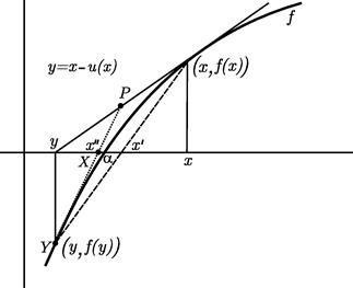
Figure 2.1 Geometric interpretation of some two-point methods
Both two-point methods (2.4) and (2.5) have cubic convergence and require three F.E. Therefore, their computational efficiency is ![]() . We also note that these methods are not optimal in the sense of the Kung-Traub conjecture (see Section 1.3) assuming that three F.E. should provide the optimal order four. The first optimal two-point method was constructed by Ostrowski (1960), several years before Traub’s extensive investigation in this area described in Traub (1964). Ostrowski’s method and its variants will be presented later, together with some other optimal methods.
. We also note that these methods are not optimal in the sense of the Kung-Traub conjecture (see Section 1.3) assuming that three F.E. should provide the optimal order four. The first optimal two-point method was constructed by Ostrowski (1960), several years before Traub’s extensive investigation in this area described in Traub (1964). Ostrowski’s method and its variants will be presented later, together with some other optimal methods.
2.1.2 Traub’s two-point methods
In his 1964’s book (Traub, 1964), Traub derived a number of cubically convergent two-point methods. One of the presented approaches relies on interpolation, which will be illustrated by several examples.
Let x be fixed and let f be a real function whose zero is sought. We construct an interpolation function ![]() such that
such that
![]() (2.6)
(2.6)
which makes use of ![]() values of functions
values of functions ![]() . The aim is to substitute the higher order derivatives by lower derivatives of f evaluated at a certain number of points. We do not require that
. The aim is to substitute the higher order derivatives by lower derivatives of f evaluated at a certain number of points. We do not require that ![]() is necessarily an algebraic polynomial. A general approach to the construction of multipoint methods of interpolatory type is presented in Traub (1964, Sec. 8.2). To construct two-point methods of third order avoiding the second derivative, we restrict ourselves to the special case when
is necessarily an algebraic polynomial. A general approach to the construction of multipoint methods of interpolatory type is presented in Traub (1964, Sec. 8.2). To construct two-point methods of third order avoiding the second derivative, we restrict ourselves to the special case when
![]() (2.7)
(2.7)
The condition ![]() is automatically fulfilled and we only impose that (2.6) holds at the point
is automatically fulfilled and we only impose that (2.6) holds at the point ![]() for
for ![]() . In this way we obtain the following system of equations
. In this way we obtain the following system of equations
![]()
This system has a solution for any ![]() . For
. For ![]() , it follows that
, it follows that ![]() , so that (2.7) becomes
, so that (2.7) becomes
![]() (2.8)
(2.8)
For ![]() there follows
there follows ![]() , and from (2.7) we get
, and from (2.7) we get
![]() (2.9)
(2.9)
Let ![]() be a zero of
be a zero of ![]() , that is,
, that is, ![]() . Putting
. Putting ![]() in (2.8), we get
in (2.8), we get
![]() (2.10)
(2.10)
This is an implicit relation in ![]() . Substituting
. Substituting ![]() by Newton’s approximation
by Newton’s approximation ![]() on the right-hand side of (2.10), we get the iteration function
on the right-hand side of (2.10), we get the iteration function
![]() (2.11)
(2.11)
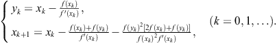
On the basis of (2.11) Traub constructed the following iterative method
![]() (2.12)
(2.12)
Note that the iterative method (2.12) was rediscovered much later by Frontini and Sormani (2003) who used the quadrature rule of midpoints
![]()
Hence
![]()
Assuming that ![]() is a zero of f, from the last relation there follows
is a zero of f, from the last relation there follows
Replacing ![]() on the right-hand side by Newton’s approximation
on the right-hand side by Newton’s approximation ![]() , one obtains Traub’s method (2.12). Note that Homeier (2003) and Özban (2004) also rediscovered this method 40 years after Traub.
, one obtains Traub’s method (2.12). Note that Homeier (2003) and Özban (2004) also rediscovered this method 40 years after Traub.
Theorem 2.1
The iterative process (2.12) has cubic convergence for sufficiently good initial approximation ![]() .
.
Proof 1
Using Taylor’s series we get
![]()
Substituting into (2.12) yields
or, after developing into Taylor’s series,
In this manner the I.F. (2.12) reduces to the Schröder basic sequence (more precisely, to the Chebyshev third-order method ![]() , see Example 1.4). Hence, according to Theorem 1.7, the iterative method (2.12) has cubic convergence. The asymptotic error constant is determined using Theorem 1.8,
, see Example 1.4). Hence, according to Theorem 1.7, the iterative method (2.12) has cubic convergence. The asymptotic error constant is determined using Theorem 1.8,
![]()
Another two-point method can be obtained from (2.9) by taking ![]() , with
, with ![]() . Then from (2.9) we get the relation
. Then from (2.9) we get the relation
![]() (2.13)
(2.13)
Replacing ![]() by
by ![]() (Newton’s approximation) on the right-hand side of (2.13), we obtain the two-point method of third order
(Newton’s approximation) on the right-hand side of (2.13), we obtain the two-point method of third order
![]() (2.14)
(2.14)
The proof of cubic convergence of the method (2.14) is similar to that of Theorem 2.1.
Traub’s method (2.14) was rediscovered many years later by Weerakoon and Fernando (2000), who derived this method by the use of numerical integration. Starting from the Newton-Leibniz formula
![]()
and applying the trapezoidal rule to estimate the definite integral
![]()
one obtains
![]()
Assuming that ![]() is a zero of f, we evaluate
is a zero of f, we evaluate ![]() from this relation and replace the argument of
from this relation and replace the argument of ![]() by some approximation
by some approximation ![]() to
to ![]() to obtain the iterative formula
to obtain the iterative formula
![]()
This is an implicit relation for ![]() . Taking
. Taking ![]() to be the argument of
to be the argument of ![]() , we get Traub’s two-point method (2.14).
, we get Traub’s two-point method (2.14).
Applying different formulae for numerical integration, some other iterative methods can be obtained. However, they usually appear to be special cases of the already existing methods.
Let us now employ the function ![]() which is inverse to f, into the interpolation formula (2.9). Then it takes the form
which is inverse to f, into the interpolation formula (2.9). Then it takes the form
![]()
For ![]() we define
we define ![]() . Then, due to the relations
. Then, due to the relations
![]()
we obtain
![]() (2.15)
(2.15)
Replacing ![]() by the approximation
by the approximation ![]() , from (2.15) there follows the iterative method of third order
, from (2.15) there follows the iterative method of third order
![]() (2.16)
(2.16)
(see Traub, 1964, p. 165). This method was later rediscovered by Homeier (2005) and Özban (2004).
A one-parameter third-order family of two-point methods
![]()
was derived by Traub, see Traub (1964, pp. 198–200). In particular, for ![]() and
and ![]() the last iterative formula generates the already presented methods (2.12) and (2.16), respectively.
the last iterative formula generates the already presented methods (2.12) and (2.16), respectively.
2.1.3 Two-point methods generated by derivative estimation
The efficiency of multipoint methods is improved by the reuse of information in every iteration. For example, it is possible to substitute higher derivatives by some suitable approximations. Here we describe Traub’s general method from which many particular methods can be derived.
Let ![]() be an I.F. function of the second order. Assume that
be an I.F. function of the second order. Assume that ![]() is of the form
is of the form
![]() (2.17)
(2.17)
where g is some function to be determined. Then ![]() , that is,
, that is, ![]() .
.
Let us take g in the form
![]()
where ![]() is a constant. The I.F. (2.17) becomes
is a constant. The I.F. (2.17) becomes
![]() (2.18)
(2.18)
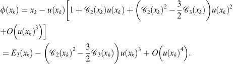
Expanding ![]() into Taylor series, we get
into Taylor series, we get
![]()
In particular, choosing ![]() where
where ![]() is a zero of f, it follows that
is a zero of f, it follows that ![]() . Consequently,
. Consequently, ![]() , which means that (2.18) defines a second-order iteration (according to Theorem 1.1). Note that
, which means that (2.18) defines a second-order iteration (according to Theorem 1.1). Note that ![]() produces the well-known quadratically convergent method of Steffensen (1933)
produces the well-known quadratically convergent method of Steffensen (1933)
![]()
Expanding the denominator in (2.18) into geometric series we arrive at the relation
![]()
Taking ![]() and having in mind that
and having in mind that ![]() , from the last relation we conclude that
, from the last relation we conclude that
![]() (2.19)
(2.19)
For this particular choice of ![]() , from (2.18) we get the I.F.
, from (2.18) we get the I.F.
![]() (2.20)
(2.20)
which is, according to (2.19), of third order. This I.F. has already been derived as a composition of Newton’s method and the secant method, see (2.5).
We will now consider approximations to the second derivative, which always appears in one-point methods of third order. Using Taylor’s series we find
 (2.21)
We recall that the third-order well-known Chebyshev method is the second member of the Schröder basic sequence
![]() (2.22)
(2.22)
Approximating ![]() by the left-hand side of (2.21), Traub derived a one-parameter family of two-step methods of third order
by the left-hand side of (2.21), Traub derived a one-parameter family of two-step methods of third order
![]() (2.23)
(2.23)
see Traub (1964, p. 181). The choice ![]() in (2.23) gives the method
in (2.23) gives the method
![]() (2.24)
(2.24)
considered later by Kou et al. (2006). The choice ![]() in (2.23) produces the method
in (2.23) produces the method
![]() (2.25)
(2.25)
rediscovered by Potra and Pták (1984). There is no essential difference between the methods (2.24) and (2.25).
Substituting ![]() in (2.21) yields the estimation to the second derivative
in (2.21) yields the estimation to the second derivative
 (2.26)
Replacing the obtained approximation into Halley’s iterative method
![]() (2.27)
(2.27)
we obtain once more the two-point I.F. of third order
![]()
Another approximation to the second derivative is by
![]()
Replacing this into the Chebyshev iterative formula (2.22) produces a one-parameter two-point family of iterative methods with cubic convergence
![]()
Its asymptotic error constant is (see Traub, 1964, p. 181)
![]()
Remark 2.1
Some of the presented two-point third-order methods can be obtained from Chun’s two-parameter family of methods derived in Chun (2007e),

where ![]() and
and ![]() .
.
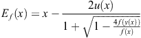
The estimation (2.26) can be suitably applied to the well-known Laguerre’s method

We first transform this into the more suitable form
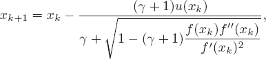 (2.28)
where we have introduced a new constant ![]() and take the sign + in front of the square root. Note that the use of the parameter
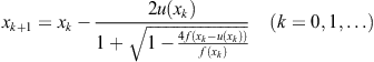
and take the sign + in front of the square root. Note that the use of the parameter ![]() transforms Laguerre’s method into Hansen-Patrick’s family, considered in Hansen and Patrick (1977). Replacing (2.26) into (2.28), we obtain a one-parameter family of two-point iterative methods
transforms Laguerre’s method into Hansen-Patrick’s family, considered in Hansen and Patrick (1977). Replacing (2.26) into (2.28), we obtain a one-parameter family of two-point iterative methods
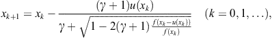 (2.29)
which was studied by Petković and Petković (2007c) and Petković et al. (1998).
Theorem 2.2
The iterative method (2.29) is of order three for all values of ![]() , and of order four for
, and of order four for ![]() .
.
Proof 2
The proof is based on Theorem 1.1. The Taylor expansion of ![]() about the point x is
about the point x is
![]() (2.30)
(2.30)
where
![]()
Then the I.F. (2.29) reads
 (2.31)
Using symbolic evaluation (say, in the computational software package Mathematica or Maple), we establish that ![]() and
and
![]() (2.32)
(2.32)
Accordingly, the order of convergence of the family of two-point methods is three for all ![]() . From (2.32) we find the asymptotic error constant
. From (2.32) we find the asymptotic error constant
![]()
It is obvious from (2.32) that for the particular value ![]() we get
we get ![]() , which means that this value of
, which means that this value of ![]() gives the two-point method of fourth order of Euler-Cauchy’s type (see (1.23)). This method reads
gives the two-point method of fourth order of Euler-Cauchy’s type (see (1.23)). This method reads
 (2.33)
and its asymptotic error constant is
![]()
Remark 2.2
The iterative method identical to (2.29) was recently rediscovered by Sharma and Guha (2011) starting from Hansen-Patrick’s method (1.25).
All methods from the two-point family (2.29) for ![]() require three F.E. per iteration and have the computational efficiency
require three F.E. per iteration and have the computational efficiency
![]()
the same one as the previously considered two-point methods and one-point cubically convergent methods presented in Section 1.5. The iterative method (2.33), obtained for ![]() , possesses the highest computational efficiency since it is of fourth order. For this method we have
, possesses the highest computational efficiency since it is of fourth order. For this method we have ![]() . We also observe that, substituting back the approximation (2.26) in (2.33), we get the third-order method
. We also observe that, substituting back the approximation (2.26) in (2.33), we get the third-order method
 (2.34)
known in the literature as Euler-Cauchy’s method.
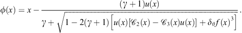
Rewrite (2.29) in the equivalent form
![]()
then it is easy to check that the limit ![]() gives the Newton-secant two-point method
gives the Newton-secant two-point method
![]() (2.35)
(2.35)
of third order, stated by Traub (1964), see (2.5).
Taking ![]() in (2.29) we obtain the method
in (2.29) we obtain the method
 (2.36)
Using the approximation (2.26), from (2.36) we find
which is the well-known square-root method or Ostrowski’s method stated by Ostrowski (1960), see also Petković and Petković (1993). Therefore, the iterative method (2.36) could be regarded as the Ostrowski-like method.
If we let ![]() in (2.29), then we obtain Newton’s method of second order. Therefore, choosing large values of
in (2.29), then we obtain Newton’s method of second order. Therefore, choosing large values of ![]() will slow down the convergence speed of the family (2.29).
will slow down the convergence speed of the family (2.29).
Example 2.4
We have compared the methods from the family (2.29) for ![]() (the fourth-order method (2.33)),
(the fourth-order method (2.33)), ![]() (method (2.36)),
(method (2.36)), ![]() (method (2.34)) and Newton’s method (
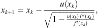
(method (2.34)) and Newton’s method (![]() ) with the two-point methods (2.12), (2.14), (2.16), and (2.24) of third order. Beside these methods, we have also tested the fourth-order method of Ostrowski (1960)
) with the two-point methods (2.12), (2.14), (2.16), and (2.24) of third order. Beside these methods, we have also tested the fourth-order method of Ostrowski (1960)
![]() (2.37)
(2.37)
developed in 1960. All tested methods require three F.E. per iteration.
We have applied the mentioned methods for finding zeros of the following six functions:
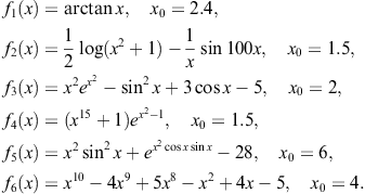
The listed functions have been tested by Mathematica in multi-precision arithmetic. The stopping criterion has been given by ![]() .
.
Let ![]() be the zero of the function
be the zero of the function ![]() . Most methods converge to the zeros
. Most methods converge to the zeros
![]()
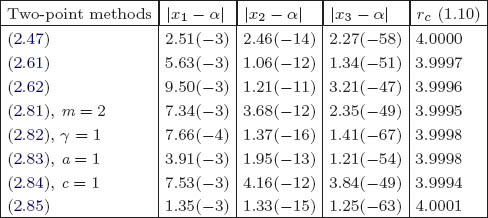
However, there are five exceptions stressed in Table 2.1 by the comments (1)–(5) and listed below the table. The term div points to the divergence and ![]() means that
means that ![]() in the kth iteration.
in the kth iteration.
Table 2.1 Results of numerical experiments
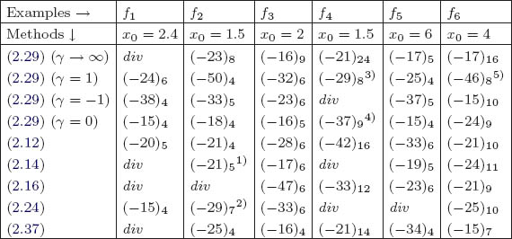
(2)![]()
(1)![]() .
.
(4)![]()
(5)![]() .
.
(3)![]()
Observe that the family (2.29) possesses the square root structure which enables finding a complex zero of real functions having conjugate complex zeros, especially in solving algebraic equations. In that case, a mathematical computation system of Mathematica automatically continues to work in complex arithmetic. The same happens when an initial approximation produces negative value under the square root. In most cases the square root methods, such as the family (2.29), overcome this difficulty producing in complex arithmetic an approximation ![]() to a real zero
to a real zero ![]() , where
, where ![]() (to the wanted accuracy) and b is a very small number in magnitude (“parasite” part) that should be neglected.
(to the wanted accuracy) and b is a very small number in magnitude (“parasite” part) that should be neglected.
We conclude this section with the comment that most of the discussed two-point methods of third order were constructed by Traub (1964) but later rediscovered by other authors. This fact was the subject of several papers, see, e.g., Chun (2007b), Chun and Neta (2009b), and Petković and Petković (2007a).
2.2 Ostrowski’s fourth-order method and its generalizations
The consideration in the previous section shows that most of the presented two-point methods possess the computational efficiency ![]() , which is equivalent to the one-point iterative methods of third order, such as Halley’s, Laguerre’s, Euler’s, or Chebyshev’s. However, since these methods require the evaluation of the first and the second derivative of a function, two-point methods are advantageous always when the evaluation of derivatives is not simple. On the other hand, if an initial approximation
, which is equivalent to the one-point iterative methods of third order, such as Halley’s, Laguerre’s, Euler’s, or Chebyshev’s. However, since these methods require the evaluation of the first and the second derivative of a function, two-point methods are advantageous always when the evaluation of derivatives is not simple. On the other hand, if an initial approximation ![]() is not sufficiently close to the sought zero, then the predictor employed in the first step (usually Newton’s approximation) cannot provide a qualitative improvement to the approximation in the second step. Figure 2.2 displays an extreme case when the sought zero is overshot due to the poor choice of the initial approximation outside of the range of convergence.
is not sufficiently close to the sought zero, then the predictor employed in the first step (usually Newton’s approximation) cannot provide a qualitative improvement to the approximation in the second step. Figure 2.2 displays an extreme case when the sought zero is overshot due to the poor choice of the initial approximation outside of the range of convergence.
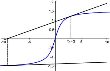
Figure 2.2 The overshooting problem of Newton’s method; ![]()
A significant advance in the construction of efficient two-point methods was achieved by two-point methods that require only three F.E. yet attain order four. This means that such methods support the Kung-Traub hypothesis (see Section 1.3) and reach optimal order of convergence. Their computational efficiency is ![]() .
.
Let ![]() be a real analytic function defined on some interval
be a real analytic function defined on some interval ![]() that contains a simple zero
that contains a simple zero ![]() of f, and let us assume that
of f, and let us assume that ![]() does not vanish on
does not vanish on ![]() . As in Section 1.3, we will use the notation
. As in Section 1.3, we will use the notation ![]() to denote the class of iteration functions
to denote the class of iteration functions ![]() which generate n-step iterative methods with the optimal order of convergence
which generate n-step iterative methods with the optimal order of convergence ![]() with fixed
with fixed ![]() . In this section we present some two-step methods of fourth order from the class
. In this section we present some two-step methods of fourth order from the class ![]() .
.
The first optimal two-point method was constructed by Ostrowski (1960), several years before Traub’s extensive investigation in this area. For its historical importance, but also for its good convergence properties, we devote a special attention to this method in this chapter. Ostrowski (1960, Ch. 11, App. G) derived his two-point method (2.37) using the interpolation of a given function f by a linear fraction
![]() (2.38)
(2.38)
at three interpolation points ![]() , and
, and ![]() , where
, where ![]() and d are constants. Let
and d are constants. Let ![]() and assume that
and assume that ![]() . It is well-known from projective geometry that if w is related to x by (2.38), then the following relation is valid,
. It is well-known from projective geometry that if w is related to x by (2.38), then the following relation is valid,
![]() (2.39)
(2.39)
that is, the points ![]() have the same cross ratio as the points
have the same cross ratio as the points ![]() . By introducing
. By introducing
![]() (2.40)
(2.40)
from (2.39) we find
![]() (2.41)
(2.41)
The function w given by (2.38) should be determined by three points ![]() so that the conditions
so that the conditions ![]() are satisfied. However, since we want to construct a two-point method using only two points, we will consider the case where two of
are satisfied. However, since we want to construct a two-point method using only two points, we will consider the case where two of ![]() coincide, for example,
coincide, for example, ![]() . We assume that
. We assume that ![]() , and
, and ![]() are known and
are known and ![]() . The corresponding interpolating function w is determined as the limit of
. The corresponding interpolating function w is determined as the limit of ![]() and (2.41) as
and (2.41) as ![]() . From (2.40) and (2.41) one obtains
. From (2.40) and (2.41) one obtains
![]() (2.42)
(2.42)
![]() (2.43)
(2.43)
It is easy to verify that ![]() satisfies the conditions
satisfies the conditions
![]()
Let ![]() . Solving (2.43) with respect to x, we get a function
. Solving (2.43) with respect to x, we get a function ![]() , implicitly expressed by
, implicitly expressed by
![]() (2.44)
(2.44)
Hence
![]() (2.45)
(2.45)
Let ![]() be a zero of f, that is,
be a zero of f, that is, ![]() . Then we can take
. Then we can take ![]() (for
(for ![]() ) as the new approximation to
) as the new approximation to ![]() . Putting
. Putting ![]() in (2.45), we obtain
in (2.45), we obtain
![]() (2.46)
(2.46)
Now let us choose ![]() to be Newton’s approximation, that is,
to be Newton’s approximation, that is,
![]()
Then from (2.42) it follows that ![]() and we get from (2.46)
and we get from (2.46)
![]()
Substituting ![]() by
by ![]() by
by ![]() , and
, and ![]() by
by ![]() , we obtain Ostrowski’s two-point method
, we obtain Ostrowski’s two-point method
 (2.47)
This iterative formula is equivalent to (2.37).
Ostrowski’s method can also be derived starting from double Newton’s method
 (2.48)
and replacing ![]() by a suitable approximation which does not require new information. Let us emphasize that (2.48) is not a proper two-point method but Newton’s method successively applied two times. In fact, we use (2.48) as an auxiliary scheme in constructing optimal two-point methods. We shall encounter similar schemes again in Chapter 4.
by a suitable approximation which does not require new information. Let us emphasize that (2.48) is not a proper two-point method but Newton’s method successively applied two times. In fact, we use (2.48) as an auxiliary scheme in constructing optimal two-point methods. We shall encounter similar schemes again in Chapter 4.
First we apply Hermite’s interpolating polynomial of second degree
![]() (2.49)
(2.49)
where the coefficients ![]() , and
, and ![]() are determined from the conditions
are determined from the conditions
![]() (2.50)
(2.50)
According to (2.50) we find
![]()
Now we obtain
![]()
and substituting ![]() yields after short arrangement
yields after short arrangement
![]() (2.51)
(2.51)
Replacing the derivative ![]() in the second step of (2.48) by
in the second step of (2.48) by ![]() given by (2.51), one obtains Ostrowski’s two-point method (2.47).
given by (2.51), one obtains Ostrowski’s two-point method (2.47).
Another derivation of Ostrowski’s method can be obtained using suitable approximations arising from Taylor’s series. Let ![]() . Since
. Since
![]()
we have
Replacing this approximation of ![]() in the second step of (2.48), we obtain (2.47).
in the second step of (2.48), we obtain (2.47).
The approximation of ![]() can be obtained by combining the Newton-Leibniz formula
can be obtained by combining the Newton-Leibniz formula
![]()
and the quadrature rule
![]()
Taking ![]() in the last quadrature formula, we obtain the system of linear equations
in the last quadrature formula, we obtain the system of linear equations

![]()
(see (2.51)). The substitution of this approximation of ![]() in (2.48) leads to the Ostrowski method (2.47).
in (2.48) leads to the Ostrowski method (2.47).
Finally, we derive Ostrowski’s method by a geometric approach using Figure 2.1. Let the point ![]() bisect the line segment determined by the points
bisect the line segment determined by the points ![]() and
and ![]() , where
, where
![]()
is Newton’s approximation. In fact, this segment is a part of the tangent line at ![]() . A new approximation
. A new approximation ![]() is the intersection of the x-axis and the secant line drawn through the points P and
is the intersection of the x-axis and the secant line drawn through the points P and ![]() (dotted line in Figure 2.1). From the similarity of the right-angle triangles (with hypotenuses
(dotted line in Figure 2.1). From the similarity of the right-angle triangles (with hypotenuses ![]() and
and ![]() ), from Figure 2.1 we observe that the equality
), from Figure 2.1 we observe that the equality
![]()
holds. Solving the last equation for ![]() , we obtain Ostrowski’s two-point method upon setting
, we obtain Ostrowski’s two-point method upon setting ![]() .
.
We have demonstrated geometric construction of Ostrowski’s method (2.47). Many new and old iterative methods can also be derived by geometric techniques. As well-known, Newton’s method may be geometrically constructed by the point of intersection of the tangent line to the graph of ![]() at the point
at the point ![]() with x-axis. Halley’s method (1.20) is geometrically interpreted by tangent hyperbolas, see Salehov (1952), while Euler-Cauchy’s method (1.23) may be derived finding the point of intersection of a quadratic parabola with x-axis, etc. Chun and Kim (2010) have used the circle of curvature, a fundamental concept in differential geometry, to derive the following third-order method of simple form,
with x-axis. Halley’s method (1.20) is geometrically interpreted by tangent hyperbolas, see Salehov (1952), while Euler-Cauchy’s method (1.23) may be derived finding the point of intersection of a quadratic parabola with x-axis, etc. Chun and Kim (2010) have used the circle of curvature, a fundamental concept in differential geometry, to derive the following third-order method of simple form,
![]()
where ![]() .
.
Chun (2007b) has developed a new I.F. geometrically, as follows. Let ![]() be a fixed parameter and let
be a fixed parameter and let ![]() be an I.F. of second order. Let
be an I.F. of second order. Let ![]() denote the intersection of the x-axis and the line passing through two points
denote the intersection of the x-axis and the line passing through two points ![]() and
and ![]() . Then
. Then
![]() (2.52)
(2.52)
The next theorem was proved in Chun (2007b).
Theorem 2.3
Let ![]() be a simple zero of f and let
be a simple zero of f and let ![]() be an I.F. of second order such that
be an I.F. of second order such that ![]() is continuous in a neighborhood of
is continuous in a neighborhood of ![]() . Then the order of the I.F.
. Then the order of the I.F. ![]() given by (2.52) is at least three when
given by (2.52) is at least three when ![]() and at least four if
and at least four if
![]()
Chun gives two examples of I.F. of fourth order. Taking Newton’s I.F. ![]() , it follows from (2.52) with
, it follows from (2.52) with ![]()
![]()
which is the Ostrowski method of fourth order (2.47). Note that the condition ![]() of Theorem 2.3 is satisfied in the case of Newton’s method so that the order four could have been predicted.
of Theorem 2.3 is satisfied in the case of Newton’s method so that the order four could have been predicted.
The second example uses quadratically convergent method
![]()
considered by Mamta et al. (2005). This method also gives ![]() and the corresponding method
and the corresponding method
![]()
is of fourth order (according to Theorem 2.3), where
![]()
Note that a two-step method of order three can be generated from (2.52) using the Newton-like I.F.
![]()
(with ![]() ).
).
Observe that Ostrowski’s method (2.47) can be obtained as a special case of many families of two-point methods developed later. This fact points that Ostrowski’s method could be regarded as an “essential method” which makes the “core” of many families of two-point methods. Since this method often gives the best results in practice in the class of methods with similar characteristics, this assertion is justified to a large extent.
Theorem 2.4
The iterative process (2.47) is of fourth order for a sufficiently close initial approximation ![]() .
.
Proof 3
From Taylor’s expansion of f, we get (omitting the argument x)
 (2.53)
According to this, we have
![]() (2.54)
(2.54)
Using (2.53) and (2.54), we obtain
![]() (2.55)
(2.55)
Taylor’s series gives
![]()
and substituting this expression back into (2.55), we obtain
![]()
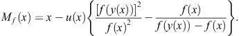
According to this, the I.F. ![]() in (2.37) can be written in the form
in (2.37) can be written in the form
![]()
To prove the fourth order of convergence of Ostrowski’s method (2.47), we use Theorem 1.8. We note that the member ![]() in Schröder’s basic sequence generated by (1.27) is given by
in Schröder’s basic sequence generated by (1.27) is given by
![]() (2.56)
(2.56)
Since ![]() when
when ![]() and
and
it follows that the limit
![]()
exists and it is not 0. In view of Theorem 1.8 it follows that Ostrowski’s two-point method (2.47) has order of convergence equal to four and the asymptotic error constant is given by
![]()
Remark 2.3
Note that Traub (1964, p. 184) gave the error relation (without proof)
![]()
pointing to the fourth order of the method (2.47). The expression on the right-hand side gives the asymptotic error constant.
Remark 2.4
According to the above consideration, we see that Ostrowski’s two-point method (2.47) belongs to the class ![]() of optimal methods of order
of optimal methods of order ![]() with 3 function evaluations. Note that good convergence behavior of Ostrowski’s method has been demonstrated by Yun and Petković (2009), where initial approximations were provided by Yun’s efficient method based on numerical integration of sigmoid-like functions; see Yun (2008) and Section 1.4.
with 3 function evaluations. Note that good convergence behavior of Ostrowski’s method has been demonstrated by Yun and Petković (2009), where initial approximations were provided by Yun’s efficient method based on numerical integration of sigmoid-like functions; see Yun (2008) and Section 1.4.
A generalization of Ostrowski’s method (2.47) was proposed by King (1973a) in the form
![]() (2.57)
(2.57)
where ![]() is a parameter. King’s family (2.57) of two-point methods is optimal and has the order four. It is easy to see that Ostrowski’s method (2.47) is a special case of (2.57) for
is a parameter. King’s family (2.57) of two-point methods is optimal and has the order four. It is easy to see that Ostrowski’s method (2.47) is a special case of (2.57) for ![]() .
.
One of several derivations of King’s family (2.57) goes as follows. We start from the expression
![]() (2.58)
(2.58)
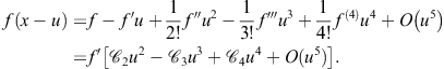
and, using (2.53) and Taylor’s series, in a similar manner as in the proof of Theorem 2.4 we find

Then we have
![]() (2.59)
(2.59)
Since the member ![]() of the Schröder basic sequences
of the Schröder basic sequences ![]() is given by
is given by
![]() (2.60)
(2.60)
(see Section 1.5), by comparing the expressions (2.59) and (2.60) we conclude that the method ![]() will reach fourth order if
will reach fourth order if ![]() . Setting
. Setting ![]() and
and ![]() in (2.58) we obtain King’s family
in (2.58) we obtain King’s family ![]() given by (2.57). Using these values of the parameters we find the asymptotic error constant
given by (2.57). Using these values of the parameters we find the asymptotic error constant
![]()
We have mentioned that Ostrowski’s method (2.47) follows from King’s family (2.57) for ![]() . The following two rediscovered optimal methods are also special cases of King’s family:
. The following two rediscovered optimal methods are also special cases of King’s family:
Remark 2.5
Some other rediscovered iterative formulae, in a less obvious form, can also be obtained from King’s family (2.57). For example, the family of two-point methods of the form
was presented by Chun and Ham (2008b). Introducing ![]() and
and ![]() , it is easy to see that this method is equivalent to King’s method (2.57).
, it is easy to see that this method is equivalent to King’s method (2.57).
Regarding the second step of (2.48) and the iterative formula (2.57), we observe that the derivative ![]() is approximated in the following way:
is approximated in the following way:
![]() (2.63)
(2.63)
Some variants of King’s family (2.57), based on different approximations to ![]() , were presented by Chun (2007c). Assuming that the quotient
, were presented by Chun (2007c). Assuming that the quotient ![]() is a reasonably small quantity, the right-hand side of (2.63) can be expanded into series
is a reasonably small quantity, the right-hand side of (2.63) can be expanded into series
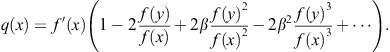 (2.64)
Taking the first three terms in (2.64) to approximate q in (2.63), Chun (2007c) obtained the family of two-point methods of fourth order,
![]() (2.65)
(2.65)
It is obvious that the family (2.65) reduces to (2.47) for ![]() .
.
Another Chun’s family (Chun, 2007a) belonging to ![]() is given by the iterative formula
is given by the iterative formula
where ![]() . Substituting
. Substituting ![]() yields the method (2.61).
yields the method (2.61).
Note that Kou et al. (2007c) derived the following two-parameter method,
and showed that this family is of third order for any ![]() . In particular, for
. In particular, for ![]() , this method attains the order four. However, in this special case the above family reduces to King’s family (2.57).
, this method attains the order four. However, in this special case the above family reduces to King’s family (2.57).
One more comment. Ostrowski’s method (2.47) can be obtained as a special case from many two-point methods belonging to the class ![]() , for instance, in the case of King’s method (2.57). Another example is the Chun-Ham family (Chun and Ham, 2007a)
, for instance, in the case of King’s method (2.57). Another example is the Chun-Ham family (Chun and Ham, 2007a)
where
![]()
and ![]() . Ostrowski’s method (2.47) is obtained for
. Ostrowski’s method (2.47) is obtained for ![]() .
.
We end this section with two methods of King-Ostrowski’s type. First we present a two-point method developed by Chun and Neta (2009b) by using the method of undetermined coefficients. Let ![]() stand for any second-order method. The iterative scheme
stand for any second-order method. The iterative scheme
![]() (2.66)
(2.66)
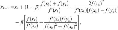
has order four, see Traub (1964), possessing the same computational efficiency as standard Newton’s method. To derive a new method of higher efficiency, Chun and Neta (2009b) have considered the expression
![]() (2.67)
(2.67)
Let ![]() . By Taylor’s series we obtain
. By Taylor’s series we obtain

Substituting the expressions on the right-hand sides of the above expansions in (2.67) and upon comparing the coefficients of f and its derivatives at ![]() , the following system of equations is obtained:
, the following system of equations is obtained:
![]()
The solution of this system is
![]()
Putting these values into (2.67), the following method follows from (2.66)
![]() (2.68)
(2.68)
where ![]() is calculated by any second-order method.
is calculated by any second-order method.
It was proved in Chun and Neta (2009b) that the order of convergence of the two-point method (2.68) is four. The iterative method (2.68) can be regarded as a generalization of Ostrowski’s method (2.47). In particular, if we take the Newton iteration as first step, that is,
![]()
then the method (2.68) reduces to the Ostrowski method (2.47).
The second method of King-Ostrowski’s type is due to Kou et al. (2007a). Combining Potra-Pták’s third-order method (Potra and Pták, 1984)
![]() (2.69)
(2.69)
and Sharma’s third-order method (Sharma, 2005)
![]() (2.70)
(2.70)
Kou et al. (2007a) stated the following one-parameter two-point method
![]() (2.71)
(2.71)
where
![]()
is Newton’s approximation and ![]() . Obviously, for
. Obviously, for ![]() formula (2.71) becomes (2.69), while the choice
formula (2.71) becomes (2.69), while the choice ![]() gives (2.70).
gives (2.70).
Other values of ![]() produce methods of third order, which are not of practical interest since they require three F.E. and attain the efficiency index
produce methods of third order, which are not of practical interest since they require three F.E. and attain the efficiency index ![]() . However, the choice
. However, the choice ![]() in (2.71) delivers the two-point method
in (2.71) delivers the two-point method
![]() (2.72)
(2.72)
of order four. The method (2.72) is a special case of King’s method setting ![]() in (2.57), see (2.61).
in (2.57), see (2.61).
2.3 Family of optimal two-point methods
In this section we present a family of two-point methods, proposed in the paper Petković and Petković (2010). Consider again the composite two-step scheme (2.48) with a reasonably good initial approximation ![]() . The presented double Newton’s scheme is simple and its rate of convergence is equal to four, which is a consequence of the fact that Newton’s method is of second order and Theorem 1.3.
. The presented double Newton’s scheme is simple and its rate of convergence is equal to four, which is a consequence of the fact that Newton’s method is of second order and Theorem 1.3.
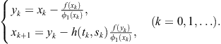
It is obvious that the computational efficiency of the iterative scheme (2.48) is the same as that of Newton’s method. This “naive” two-step method requires four F.E. per iteration. To reduce the number of evaluations and thus increase the computational efficiency, Chun (2008) introduced a useful technique for approximating the first derivative using a suitably chosen weight function h,
![]()
where ![]() . Here h is a real-valued function to be chosen so that the two-point method
. Here h is a real-valued function to be chosen so that the two-point method
 (2.73)
is of order four. Chun showed that any function h, satisfying ![]() , and
, and ![]() , provides the fourth order of the two-point iterative scheme (2.73).
, provides the fourth order of the two-point iterative scheme (2.73).
The presented idea is both simple and fruitful. Sometimes it is necessary to develop the function h into Taylor’s or geometric series to generate suitable (both new and existing) iteration functions. Chun (2008) listed the following examples:
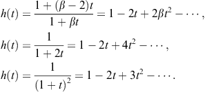
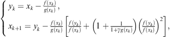
A slightly more direct approach without altering the weight function, considered in Petković and Petković (2010), is based on Chun’s idea to approximate ![]() by
by
![]()
assuming that a real-weight function g and its derivatives ![]() and
and ![]() are continuous in the neighborhood of 0. Now the two-step scheme (2.48) becomes
are continuous in the neighborhood of 0. Now the two-step scheme (2.48) becomes
 (2.74)
The weight function g in (2.74) has to be determined so that the two-point method (2.74) attains the optimal order four using only three function evaluations: ![]() , and
, and ![]() . This is the subject of the following theorem (see Petković and Petković, 2010).
. This is the subject of the following theorem (see Petković and Petković, 2010).
Theorem 2.5
Let ![]() be a simple zero of a real single-valued function
be a simple zero of a real single-valued function ![]() possessing a certain number of continuous derivatives in the neighborhood of
possessing a certain number of continuous derivatives in the neighborhood of ![]() , where
, where ![]() is an open interval. Let g be a function satisfying
is an open interval. Let g be a function satisfying ![]() and
and ![]() . If
. If ![]() is sufficiently close to
is sufficiently close to ![]() , then the order of convergence of the family of two-step methods (2.74) is four and the error relation
, then the order of convergence of the family of two-step methods (2.74) is four and the error relation
![]() (2.75)
(2.75)
holds.
Proof 4
Let ![]() as before and let us introduce the errors
as before and let us introduce the errors
![]()
Expanding f into Taylor’s series about ![]() , we find
, we find
![]() (2.76)
(2.76)
Hence, applying again Taylor’s series to ![]() , we get
, we get
![]() (2.77)
(2.77)
Furthermore, we have
![]() (2.78)
(2.78)
Let us approximate the function g by its Taylor’s polynomial of second degree at the point ![]() ,
,
![]() (2.79)
(2.79)
Now, using (2.76)–(2.79), we find for ![]()
Substituting the conditions ![]() and
and ![]() of the theorem in the expression for
of the theorem in the expression for ![]() , we obtain
, we obtain
![]()
which is exactly the error relation (2.75). Hence we conclude that the order of the family (2.74) is four. ![]()
Remark 2.6
From (2.75) we notice that the asymptotic error constant of the method (2.74) is
![]()
To determine the corresponding expression of the asymptotic error constant in the case of a particular method obtained by choosing a specific function g, it is necessary to find ![]() and substitute this value in the above expression. For example, for King’s method (2.57) we have
and substitute this value in the above expression. For example, for King’s method (2.57) we have
![]()
and hence ![]() .
.
We give some special cases of the two-point family (2.74) of methods. This family produces a variety of new methods as well as some existing optimal two-point methods which appear as special cases. The chosen function g in the subsequent examples satisfies the conditions ![]() and
and ![]() , given in Theorem 2.5. We write
, given in Theorem 2.5. We write ![]() for short.
for short.
Method 2.1. For g given by
![]()
we obtain King’s fourth-order family of two-point methods given by (2.57). Recall that King’s family produces as special cases Ostrowski’s method (2.47)![]() , Kou-Li-Wang’s method (2.61)
, Kou-Li-Wang’s method (2.61)![]() and Chun’s method (2.62)
and Chun’s method (2.62)![]() .
.
Method 2.2. Choosing g in the form
![]()
one obtains a family of fourth-order methods
![]() (2.80)
(2.80)
Taking ![]() in (2.80) we get Chun’s method (2.62), while the choice
in (2.80) we get Chun’s method (2.62), while the choice ![]() gives Ostrowski’s method (2.47). The choice
gives Ostrowski’s method (2.47). The choice ![]() gives the iterative method
gives the iterative method
![]() (2.81)
(2.81)
Method 2.3. For g defined by
![]()
we obtain a one-parameter family of two-point methods
![]() (2.82)
(2.82)
Substituting ![]() in (2.82) yields Ostrowski’s method (2.47).
in (2.82) yields Ostrowski’s method (2.47).
Method 2.4. The choice
![]()
gives a family of optimal two-point methods defined by the I.F.
 (2.83)
Ostrowski’s method (2.47) is obtained as a special case putting ![]() in (2.83). In fact, the method (2.83) is Chun’s method (2.65) with
in (2.83). In fact, the method (2.83) is Chun’s method (2.65) with ![]() .
.
Method 2.5. Choosing
![]()
we construct the I.F.
![]() (2.84)
(2.84)
which defines a one-parameter family of two-point methods ![]() of order four. Taking
of order four. Taking ![]() in (2.84), we obtain Maheshwari’s method (Maheshwari, 2009) as a special case,
in (2.84), we obtain Maheshwari’s method (Maheshwari, 2009) as a special case,
 (2.85)
Method 2.6. The weight function
![]()
satisfies the conditions of Theorem 2.5 in a limit case when ![]() and produces the fourth-order method of Euler-Cauchy’s type
and produces the fourth-order method of Euler-Cauchy’s type
 (2.86)
proposed in Petković and Petković (2007c) and already discussed in Section 2.1, see (2.33).
Remark 2.7
Cordero et al. (2010) presented the optimal two-point fourth-order method in the form
This method is referred to as modified Potra-Pták method after Potra-Pták method (2.25). However, the above two-point method is a special case of the family (2.74) for ![]() . Moreover, the addend
. Moreover, the addend ![]() , which follows after
, which follows after ![]() in the second step, can be omitted (that is, taking
in the second step, can be omitted (that is, taking ![]() ) preserving order four. Then the second step takes a simple form
) preserving order four. Then the second step takes a simple form
![]()
which can be obtained from Ostrowski’s method (2.47) by approximating ![]() .
.
Example 2.5
The convergence behavior of some optimal two-point methods, considered in this section, has been tested using the function
![]()
for finding its zero ![]() which lies in the interval [2,5]. We have chosen the initial approximation
which lies in the interval [2,5]. We have chosen the initial approximation ![]() . The computational software package Mathematica with multi-precision arithmetic has been employed.
. The computational software package Mathematica with multi-precision arithmetic has been employed.
Table 2.2 contains absolute values of the errors of approximations in the first three iterations, where ![]() means
means ![]() . This table also contains the entries of the computational order of convergence, evaluated by (1.10).
. This table also contains the entries of the computational order of convergence, evaluated by (1.10).
Table 2.2 Example 2.5 – ![]()
2.4 Optimal derivative free two-point methods
In many real-life problems it is preferable to avoid calculations of derivatives of f. The classical Steffensen’s method (Steffensen, 1933)
![]() (2.87)
(2.87)
derived from Newton’s method
![]()
by substituting the derivative ![]() with the ratio
with the ratio
![]()
is an example of a derivative free root-finding method. The efficiency index of Steffensen’s method is ![]() , the same as that of Newton’s method.
, the same as that of Newton’s method.
In this section we consider a family of derivative free two-point methods without memory of order four. Its variant with memory is studied in Chapter 6. Some of the presented results are studied in Petković et al. (2010c). In general, derivative free methods are useful for finding zeros of a function f when the calculation of derivatives of f is complicated and expensive.
Let
![]()
where ![]() is an arbitrary real constant. Upon expanding
is an arbitrary real constant. Upon expanding ![]() into Taylor’s series about x, we arrive at
into Taylor’s series about x, we arrive at
![]()
Hence, we obtain an approximation to the derivative ![]() in the form
in the form
![]() (2.88)
(2.88)
studied many years ago in Traub (1964, p. 178).
To construct derivative free two-point methods of optimal order, let us start from the double Newton’s method (2.48). It is well-known that the iterative scheme (2.48) is inefficient and our primary aim is to improve its computational efficiency. We also wish to substitute derivatives ![]() and
and ![]() in (2.48) by convenient approximations. This replacement can be carried out at the first step using the approximation (2.88) to
in (2.48) by convenient approximations. This replacement can be carried out at the first step using the approximation (2.88) to ![]() . The derivative
. The derivative ![]() in the second step of (2.48) will be approximated by
in the second step of (2.48) will be approximated by ![]() , where
, where ![]() is a differentiable function that depends on two real variables
is a differentiable function that depends on two real variables
![]()
Therefore,
![]() (2.89)
(2.89)
![]() (2.90)
(2.90)
Starting from the iterative scheme (2.48) and using (2.89) and (2.90), we construct the following family of two-point methods (Petković et al., 2010c)
 (2.91)
The weight function h should be determined in such a way to provide the fourth order of convergence of the two-point method (2.91).
Let ![]() denote the error of approximation calculated in the kth iteration. In our convergence analysis we will omit sometimes the iteration index k for simplicity. A new approximation
denote the error of approximation calculated in the kth iteration. In our convergence analysis we will omit sometimes the iteration index k for simplicity. A new approximation ![]() to the root
to the root ![]() will be denoted with
will be denoted with ![]() . Let us introduce the errors
. Let us introduce the errors
![]()
We will use Taylor’s expansion about the root ![]() to express
to express ![]() , and
, and ![]() as series in
as series in ![]() . Then we represent
. Then we represent ![]() and
and ![]() by Taylor’s polynomials in
by Taylor’s polynomials in ![]() .
.
Assume that x is sufficiently close to the zero ![]() of f, then s and t are very small quantities in magnitude. Let us represent a real function of two variables h appearing in (2.91) by Taylor’s series about (0, 0) in a linear form,
of f, then s and t are very small quantities in magnitude. Let us represent a real function of two variables h appearing in (2.91) by Taylor’s series about (0, 0) in a linear form,
![]() (2.92)
(2.92)
where ![]() and
and ![]() denote partial derivatives of h with respect to t and s. It can be proved that the use of partial derivatives of higher order does not provide faster convergence (greater than four) of two-point methods without memory.
denote partial derivatives of h with respect to t and s. It can be proved that the use of partial derivatives of higher order does not provide faster convergence (greater than four) of two-point methods without memory.
Expressions of Taylor’s polynomials (in ![]() ) of functions involved in (2.91) are cumbersome and lead to tedious calculations, which requires the use of a computer. If a computer is employed anyway, it is reasonable to perform all calculations necessary in finding the convergence rate using symbolic computation, as done in what follows. Such an approach was used in Thukral and Petković (2010) and later papers. Therefore, instead of presenting explicit expressions in the convergence analysis we use symbolic computation in Mathematica to find candidates for h. If necessary, intermediate expressions can always be displayed during this computation using the program given below, although their presentation is most frequently of academic interest.
) of functions involved in (2.91) are cumbersome and lead to tedious calculations, which requires the use of a computer. If a computer is employed anyway, it is reasonable to perform all calculations necessary in finding the convergence rate using symbolic computation, as done in what follows. Such an approach was used in Thukral and Petković (2010) and later papers. Therefore, instead of presenting explicit expressions in the convergence analysis we use symbolic computation in Mathematica to find candidates for h. If necessary, intermediate expressions can always be displayed during this computation using the program given below, although their presentation is most frequently of academic interest.
We will find the coefficients ![]() of the expansion (2.92) using a simple program in Mathematica and an interactive approach explained by the comments C1, C2, and C3. First, let us introduce abbreviations used in this program.
of the expansion (2.92) using a simple program in Mathematica and an interactive approach explained by the comments C1, C2, and C3. First, let us introduce abbreviations used in this program.
Program (written in Mathematica)
fx = f1a∗(e + c2∗eˆ2 + c3∗eˆ3 + c4∗eˆ4);
fxi = f1a∗((e + g∗fx)+c2∗(e + g∗fx)ˆ2 + c3∗(e + g∗fx)ˆ3);
fi = Series[(fxi-fx)/(g∗fx),{e,0,2}];
ey = e-g∗fxˆ2∗Series[1/(fxi-fx),{e,0,2}];
fy = f1a∗(ey + c2∗eyˆ2 + c3∗eyˆ3);
e1 = ey-(h0 + ht∗t + hs∗s)∗Series[fy/fi,{e,0,3}]//Simplify;
Out[A2]= c2(1 + g f1a)(1-h0)
h0 = 1; A3 = Coefficient[e1,eˆ3]//Simplify
Out[A3]=![]() (2+
(2+![]() (1-ht)-ht-hs-g f1a (-3 + 2ht + hs))
(1-ht)-ht-hs-g f1a (-3 + 2ht + hs))
ht = 1; hs = 1; A4 = Coefficient[e1,eˆ4]//Simplify
Out[A4]=![]()
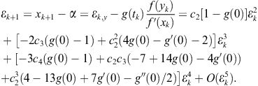
Comment C1: From the expression for the error ![]() we observe that
we observe that ![]() is of the form
is of the form
![]() (2.93)
(2.93)
The iterative two-point method (2.91) will have order four if the coefficients of the expansion (2.92) are chosen so that ![]() and
and ![]() (in (2.93)) vanish. We find these coefficients equating shaded expressions in the boxed formulae to 0. First, from Out[A2] we set
(in (2.93)) vanish. We find these coefficients equating shaded expressions in the boxed formulae to 0. First, from Out[A2] we set ![]() and then calculate
and then calculate ![]() .
.
Comment C2: From Out[A3] we see that the term ![]() can be eliminated only if we choose
can be eliminated only if we choose ![]() . With this value the coefficient
. With this value the coefficient ![]() will vanish if we take
will vanish if we take ![]() .
.
Comment C3: Substituting the entries ![]() in the expression of e1 (
in the expression of e1 (![]() ), we obtain
), we obtain

or, using the iteration index,
 (2.94)
Therefore, to provide the fourth-order of convergence of the two-point methods (2.91), it is necessary to choose the function of two variables h so that its truncated expansion (2.92) satisfies
![]() (2.95)
(2.95)
According to the above analysis we can formulate the following convergence theorem.
Theorem 2.6
Let ![]() be a differentiable function of two variables that satisfies the conditions
be a differentiable function of two variables that satisfies the conditions ![]() . If an initial approximation
. If an initial approximation ![]() is sufficiently close to a zero
is sufficiently close to a zero ![]() of a function f, then the order of the family of two-point methods (2.91) is equal to four.
of a function f, then the order of the family of two-point methods (2.91) is equal to four.
Let us study the choice of the weight function h in (2.91). Considering (2.95), we see that the simplest form of h is obviously
![]() (2.96)
(2.96)
Note that any function of the form ![]() , where g is a differentiable function such that
, where g is a differentiable function such that ![]() , satisfies the condition (2.95). For example, we can take
, satisfies the condition (2.95). For example, we can take ![]() (
(![]() is a parameter),
is a parameter), ![]() , and so on. The two-parameter function
, and so on. The two-parameter function ![]() also satisfies the condition (2.95).
also satisfies the condition (2.95).
Other examples of usable functions are as follows:
![]() (2.97)
(2.97)
![]() (2.98)
(2.98)
![]() (2.99)
(2.99)
![]() (2.100)
(2.100)
It is easy to check that these functions satisfy the conditions (2.95).
Remark 2.8
The family of two-point methods (2.91) requires three F.E. and has order of convergence four. Therefore, this family is optimal in the sense of the Kung-Traub conjecture and possesses the computational efficiency ![]() .
.
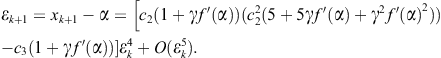
Remark 2.9
According to (2.94), we find the asymptotic error constant

However, this expression is valid if the Taylor series of h is truncated to the polynomial form (2.96). For any other particular function h, the asymptotic error constant takes a specific expression. For example, choosing ![]() (formula (2.97)) we find the asymptotic error constant
(formula (2.97)) we find the asymptotic error constant
![]()
Remark 2.10
We speak about the family (2.91) since the choice of the free parameter ![]() and various weight functions h, satisfying the conditions (2.95), provides a variety of two-point methods.
and various weight functions h, satisfying the conditions (2.95), provides a variety of two-point methods.
Remark 2.11
Peng et al. (2011) displayed (without derivation) the following derivative free two-point method of fourth order,
where ![]() coincides with
coincides with ![]() given by (2.88) and
given by (2.88) and ![]() is a real parameter. It is easy to show that this method is a special case of the family (2.91) with the basic choice
is a real parameter. It is easy to show that this method is a special case of the family (2.91) with the basic choice
![]()
Remark 2.12
Sharma and Goyal (2006) have shown that the derivative free two-point method
where
![]()
has order four. To avoid any additional calculations, it is preferable to choose ![]() as a constant. Therefore, without loss of generality, we can adopt that
as a constant. Therefore, without loss of generality, we can adopt that ![]() The Sharma-Goyal method can be obtained from the family (2.91) taking
The Sharma-Goyal method can be obtained from the family (2.91) taking
![]()
and ![]() in (2.88), providing
in (2.88), providing ![]() . Moreover, the family (2.91), with
. Moreover, the family (2.91), with ![]() chosen as above, can deal with arbitrary
chosen as above, can deal with arbitrary ![]() , that is, we may replace
, that is, we may replace ![]() by
by ![]() given by (2.88).
given by (2.88).
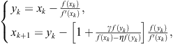
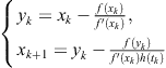
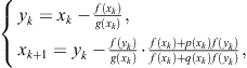
Now we will present a derivative free two-point method of optimal order four related to the family (2.91). Starting from the Steffensen-Newton scheme
 (2.101)
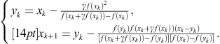
of fourth order, Ren et al. (2009) eliminated ![]() using only available information. In this way, they derived a two-point method of order four costing three function evaluations. Using an interpolating polynomial
using only available information. In this way, they derived a two-point method of order four costing three function evaluations. Using an interpolating polynomial
![]()
and the conditions
![]() (2.102)
(2.102)
where ![]() , the following approximation is obtained:
, the following approximation is obtained:
![]() (2.103)
(2.103)
Here ![]() is an arbitrary parameter. Substituting (2.103) into (2.101), the derivative free two-point method of the form
is an arbitrary parameter. Substituting (2.103) into (2.101), the derivative free two-point method of the form
 (2.104)
was stated and the following theorem was proved in Ren et al. (2009).
Theorem 2.7
(Ren et al., 2009) Let ![]() be a simple zero of a sufficiently differentiable function
be a simple zero of a sufficiently differentiable function ![]() for an open interval
for an open interval ![]() . If
. If ![]() is sufficiently close to
is sufficiently close to ![]() , then the class of methods defined by (2.104) is of fourth order, and satisfies the error relation
, then the class of methods defined by (2.104) is of fourth order, and satisfies the error relation
![]() (2.105)
(2.105)
Observe from the error relation (2.105) that the parameter a does not influence the order of convergence considering (2.104) as a method without memory. This is also clear from the estimations
![]()
Namely, the term ![]() in the denominator of (2.104) is of higher order and can be neglected. This is equivalent to the choice
in the denominator of (2.104) is of higher order and can be neglected. This is equivalent to the choice ![]() in the iterative scheme (2.104). Practical examples justify such conclusion. Finally, note that the approximation (2.103) with
in the iterative scheme (2.104). Practical examples justify such conclusion. Finally, note that the approximation (2.103) with ![]() can be obtained using Newtonian interpolation, see (2.107).
can be obtained using Newtonian interpolation, see (2.107).
Remark 2.13
Regarding (2.105), a modified method with slightly improved convergence order could be constructed calculating ![]() . It is assumed that
. It is assumed that ![]() , and
, and ![]() are approximated using data from the previous and current iteration. However, this approach is rather artificial and awkward and gives only slight acceleration of convergence. More efficient accelerating methods are studied in Chapter 6.
are approximated using data from the previous and current iteration. However, this approach is rather artificial and awkward and gives only slight acceleration of convergence. More efficient accelerating methods are studied in Chapter 6.
Let us compare the Ren-Wu-Bi method (2.104) with ![]() and the family (2.91) with
and the family (2.91) with ![]() . The first step for both methods is the Steffensen method (2.87). The second step of (2.104)a=0 may be written in the form
. The first step for both methods is the Steffensen method (2.87). The second step of (2.104)a=0 may be written in the form

where ![]() is the already mentioned function (2.99) and
is the already mentioned function (2.99) and ![]() is given by (2.88) for
is given by (2.88) for ![]() . Therefore, the Ren-Wu-Bi method (2.104) for
. Therefore, the Ren-Wu-Bi method (2.104) for ![]() can be derived from the family (2.91) as a special case for
can be derived from the family (2.91) as a special case for
![]()
This also means that a simpler interpolation function of the form
![]()
and the conditions (2.102) can be used for the approximation of ![]() in (2.103). It is easy to check that the two-point method (2.104)a=0 is obtained in this manner.
in (2.103). It is easy to check that the two-point method (2.104)a=0 is obtained in this manner.
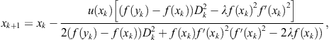
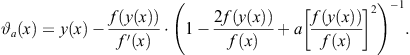
Cordero and Torregrosa (2011) approximated the derivative ![]() in the Steffensen-Newton scheme (2.101) in the following way,
in the Steffensen-Newton scheme (2.101) in the following way,
![]()
where ![]() , and
, and ![]() are real parameters. They proved that the obtained derivative free family of two-point methods is of order four if
are real parameters. They proved that the obtained derivative free family of two-point methods is of order four if ![]() and
and ![]() and the error relation
and the error relation
![]()
holds. However, it is easy to show that this method is only a special case of Ren-Wu-Bi’s family (2.104) for ![]() . Consequently, the above error relation reduces to (2.105) for
. Consequently, the above error relation reduces to (2.105) for ![]() .
.
An additional observation about the Ren-Wu-Bi method (2.104) for ![]() . This special case has appeared as a starting point in developing a new method in the paper of Liu et al. (2010). Namely, having in mind that
. This special case has appeared as a starting point in developing a new method in the paper of Liu et al. (2010). Namely, having in mind that
![]()
Liu et al. (2010) use a simple approximation of the form ![]() (for small
(for small ![]() ) and find
) and find
Returning back into ![]() yields the derivative free two-point fourth-order method,
yields the derivative free two-point fourth-order method,
From the previous consideration we can observe that several methods for constructing two-point methods have been used: interpolation by bilinear function, Hermite’s interpolation, approximation of the derivative, interpolating polynomials. We shall deal with inverse interpolation in Section 2.5. Now we demonstrate another approach based on Newton’s interpolation with divided differences. Let the first step in (2.48) be represented by Steffensen’s method (2.87). We calculate the next approximation by
![]() (2.106)
(2.106)
![]()
is Newton’s interpolating polynomial of second degree that satisfies the conditions
![]()
where ![]() . Hence
. Hence
![]() (2.107)
(2.107)
Using (2.87) and (2.107), the following two-point method is stated
 (2.108)
In this manner we derived the Ren-Wu-Bi method (2.104) for ![]() . The iterative method (2.108) can also be obtained as a special case of the family (2.91) for
. The iterative method (2.108) can also be obtained as a special case of the family (2.91) for ![]() and
and ![]() .
.
2.5 Kung-Traub’s multipoint methods
A fundamental and one of the most influential papers in the topic of multipoint methods for solving nonlinear equations is certainly Kung-Traub’s paper (Kung and Traub, 1974). Aside from the famous conjecture on the upper bound of the order of convergence of multipoint methods with fixed number of F.E. (see Section 1.3), this paper presents two optimal multipoint families of iterative methods of arbitrary order. These general families will be studied in later chapters together with their convergence analysis. However, frequent use and citation of these families, called K-T family for brevity, imposes their short introduction. We present Kung-Traub’s families in the form given in Kung and Traub (1974).
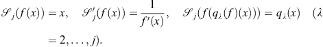
K-T (2.109): For any m, define iteration function ![]() as follows:
as follows: ![]() and for
and for ![]() ,
,
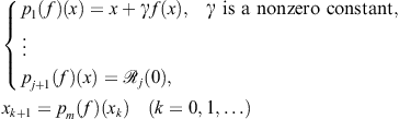 (2.109)
for ![]() , where
, where ![]() is the inverse interpolating polynomial of degree at most j such that
is the inverse interpolating polynomial of degree at most j such that
![]()
Let us note that the family K-T (2.109) requires no evaluation of derivatives of f. The order of convergence of the family K-T (2.109), consisting of ![]() steps, is
steps, is ![]() .
.
K-T (2.110): For any m, define iteration function ![]() as follows:
as follows: ![]() , and for
, and for ![]() ,
,
 (2.110)
for ![]() , where
, where ![]() is the inverse interpolating polynomial of degree at most j such that
is the inverse interpolating polynomial of degree at most j such that
The order of convergence of the family K-T (2.110), consisting of ![]() steps, is
steps, is ![]() .
.
Remark 2.14
![]() in (2.109) and
in (2.109) and ![]() in (2.110) are only initializing steps and they do not make the first step of the described iterations.
in (2.110) are only initializing steps and they do not make the first step of the described iterations.
In this chapter we study two-point methods so that it is of interest to present two-point methods obtained as special cases of the Kung-Traub families (2.109) and (2.110). First, for ![]() we obtain from (2.109) the derivative free two-point method
we obtain from (2.109) the derivative free two-point method
 (2.111)
The two-point method (2.111) is of fourth order and requires three F.E. so that it belongs to the class ![]() of optimal methods.
of optimal methods.
The iterative scheme (2.111) can be rewritten in the form
 (2.112)
where ![]() and
and ![]() . Comparing (2.112) to (2.91) with h given by (2.98), we observe that the family (2.91) is a generalization of the Kung-Traub two-point method (2.111).
. Comparing (2.112) to (2.91) with h given by (2.98), we observe that the family (2.91) is a generalization of the Kung-Traub two-point method (2.111).
Taking ![]() in (2.110), we obtain Kung-Traub’s two-point method of fourth order,
in (2.110), we obtain Kung-Traub’s two-point method of fourth order,
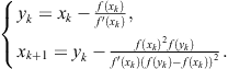 (2.113)
Note that the family (2.74) is a generalization of Kung-Traub’s method (2.113), which follows from this family taking ![]() in (2.80) or
in (2.80) or ![]() in (2.83).
in (2.83).
Example 2.6
We have applied some of the presented two-point methods of fourth order to the function
![]()
to approximate its zero ![]() . In this test we have used the common initial approximation
. In this test we have used the common initial approximation ![]() . The absolute values of the errors of approximations
. The absolute values of the errors of approximations ![]() in the first four iterations are displayed in Table 2.3.
in the first four iterations are displayed in Table 2.3.
Table 2.3 Example 2.6 – ![]()
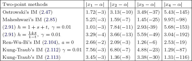
2.6 Optimal two-point methods of Jarratt’s type
Most of the multipoint methods presented in this book use two or more evaluations of a given function f at different points and only one evaluation of ![]() . After Ostrowski’s two-point method (2.47) of optimal order four (Ostrowski, 1960), constructed in 1960, the next two-point method of fourth order was derived by Jarratt (1966). Jarratt’s approach relies on an extended Traub’s form investigated in Traub (1964) and uses one function and two derivative evaluations per iteration. For this reason, optimal two-point methods with such a model of evaluation are often called methods of Jarratt’s type. It is worth noting that, among two-point methods, only Jarratt’s model possesses (at present) the feature to generate two-point methods of optimal order four for finding multiple roots (see Section 2.7).
. After Ostrowski’s two-point method (2.47) of optimal order four (Ostrowski, 1960), constructed in 1960, the next two-point method of fourth order was derived by Jarratt (1966). Jarratt’s approach relies on an extended Traub’s form investigated in Traub (1964) and uses one function and two derivative evaluations per iteration. For this reason, optimal two-point methods with such a model of evaluation are often called methods of Jarratt’s type. It is worth noting that, among two-point methods, only Jarratt’s model possesses (at present) the feature to generate two-point methods of optimal order four for finding multiple roots (see Section 2.7).
2.6.1 Jarratt’s two-step methods
Let us define the functions
![]()
Traub showed in Traub (1964, pp. 197–204) that iterative formulae of the type
![]() (2.114)
(2.114)
can reach cubic order of convergence by suitable choices of the parameters ![]() , and
, and ![]() , costing one evaluation of
, costing one evaluation of ![]() and two of
and two of ![]() per iteration. Further acceleration of convergence of (2.114) is not possible without increasing the number of F.E.
per iteration. Further acceleration of convergence of (2.114) is not possible without increasing the number of F.E.
In his paper (Jarratt, 1966) Jarratt examined a similar class of iterative methods of the form
![]() (2.115)
(2.115)
where
![]()
Jarratt succeeded in increasing the order of convergence of (2.115) from three to four without additional F.E., contrary to Traub’s iterative formulae (2.114) of third order.
Let ![]() be a zero of f and let
be a zero of f and let ![]() be the error in the kth iteration. Sometimes we will write
be the error in the kth iteration. Sometimes we will write ![]() instead of
instead of ![]() and omit the argument of u for simplicity. Using the Taylor expansions of
and omit the argument of u for simplicity. Using the Taylor expansions of ![]() and
and ![]() about the zero
about the zero ![]() , we find
, we find
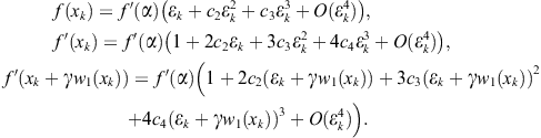
Since
![]() (2.116)
(2.116)
![]() (2.117)
(2.117)
After tedious but elementary calculations, from (2.116) and (2.117) one obtains
![]() (2.118)
(2.118)
and
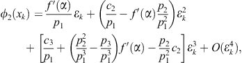 (2.119)
where the abbreviations
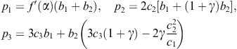
are used. Now we substitute (2.118) and (2.119) into (2.115) and after collecting terms in ![]() , the error relation of the form
, the error relation of the form
![]()
is obtained.
The coefficients ![]() , and
, and ![]() depend on
depend on ![]() , and
, and ![]() . The expressions for these coefficients are rather lengthy and will not be given explicitly. The iterative method (2.115) will reach fourth order only if
. The expressions for these coefficients are rather lengthy and will not be given explicitly. The iterative method (2.115) will reach fourth order only if ![]() . To satisfy these conditions, the following system of equations must be fulfilled (see Jarratt, 1966):
. To satisfy these conditions, the following system of equations must be fulfilled (see Jarratt, 1966):
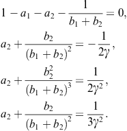
For consistency of the second and last equation we must choose ![]() so that the above system reduces to
so that the above system reduces to
![]() (2.120)
(2.120)
![]() (2.121)
(2.121)
![]() (2.122)
(2.122)
where we set ![]() for convenience. The restrictions
for convenience. The restrictions ![]() are necessary since
are necessary since ![]() gives
gives ![]() while
while ![]() leads to
leads to ![]() . In both cases (2.115) degenerate to (2.114) and the fourth order cannot be achieved.
. In both cases (2.115) degenerate to (2.114) and the fourth order cannot be achieved.
Assuming that ![]() , the general solution of the system (2.122) in terms of
, the general solution of the system (2.122) in terms of ![]() is
is

In this way Jarratt constructed a general family of fourth-order two-point methods requiring only one function and two derivative evaluations per iteration,
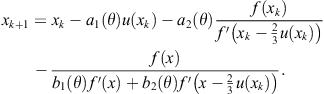 (2.123)
Therefore, Jarratt’s family (2.123) is optimal in the sense of the Kung-Traub conjecture.
The parameter ![]() in (2.123) should be chosen so that the form of (2.123) is as simple as possible. The following three particular methods were presented in Jarratt’s paper (Jarratt, 1966) putting
in (2.123) should be chosen so that the form of (2.123) is as simple as possible. The following three particular methods were presented in Jarratt’s paper (Jarratt, 1966) putting ![]() for short:
for short:
![]() (2.124)
(2.124)
![]() (2.125)
(2.125)
![]() (2.126)
(2.126)
Jarratt applied a similar approach in Jarratt (1969) to construct a two-point method of fourth order consuming one function and two derivative evaluations per iteration. He searched for efficient I.F. in the form
![]() (2.127)
(2.127)
where ![]() and
and ![]() are given by (2.116) and (2.117). To determine the coefficients
are given by (2.116) and (2.117). To determine the coefficients ![]() , and
, and ![]() in (2.127), Jarratt used the Schröder basic sequence (1.27). Recall that two iterative methods of order p can only differ by terms proportional to
in (2.127), Jarratt used the Schröder basic sequence (1.27). Recall that two iterative methods of order p can only differ by terms proportional to ![]() or higher, see Theorem 1.7. By comparing
or higher, see Theorem 1.7. By comparing ![]() and the fifth-order method
and the fifth-order method ![]() given by (2.56), Jarratt arrived at the following difference (with the parameter
given by (2.56), Jarratt arrived at the following difference (with the parameter ![]() renamed to
renamed to ![]() )
)
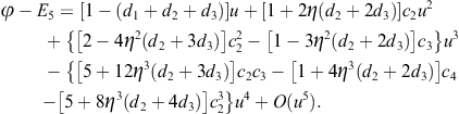 (2.128)
The I.F. ![]() will reach fourth order if the coefficients of
will reach fourth order if the coefficients of ![]() , and
, and ![]() all vanish for arbitrary function
all vanish for arbitrary function ![]() . These conditions lead to the following system of equations obtained from (2.128):
. These conditions lead to the following system of equations obtained from (2.128):
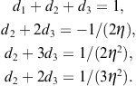 (2.129)
Similarly as in the case of Jarratt’s family (2.123), the second and last equations will be consistent only if ![]() . With this value, the system (2.129) reduces to
. With this value, the system (2.129) reduces to
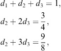
with the solution ![]() . In view of (2.127), the two-point method gets the simple form
. In view of (2.127), the two-point method gets the simple form
![]() (2.130)
(2.130)
Let us return to Jarratt’s method (2.124) and rewrite it in the form
![]() (2.131)
(2.131)
where
![]()
If x is sufficiently close to a zero of f, then ![]() is small and we have
is small and we have ![]() . Then the expansion in geometric series gives
. Then the expansion in geometric series gives
![]()
Substituting this into (2.131) yields the iterative formula of order four
![]() (2.132)
(2.132)
This two-point method is often called inverse-free Jarratt’s method, see, e.g., Amat et al. (2004) and Varona (2002). These cited papers present the convergence behavior of the inverse-free Jarratt method (2.132) and several other methods from a dynamical point of view, using a graphic visualization by fractal pictures. Comparing the iterative formulae (2.124) and (2.132) it might look at first glance that the inverse has been eliminated. However, this is not quite correct since ![]() contains
contains ![]() , which is a drawback if (2.132) is applied to systems of nonlinear equations.
, which is a drawback if (2.132) is applied to systems of nonlinear equations.
Remark 2.15
Note that the methods (2.123), (2.130), and (2.132) of Jarratt’s type use in the first step a specific approximation ![]() (with
(with ![]() ), contrary to most multi-step methods that employ Newton’s approximation
), contrary to most multi-step methods that employ Newton’s approximation ![]() (with
(with ![]() ). The former will be called Jarratt’s step to differ from the latter Newton’s step.
). The former will be called Jarratt’s step to differ from the latter Newton’s step.
A family of two-point methods of fourth order, which also uses one function and two derivative evaluations as Jarratt’s methods (2.123), (2.130), and (2.132), has been proposed in Chun and Ham (2008a). The base for constructing this family is the third-order method
![]() (2.133)
(2.133)
often called super-Halley’s method, where
![]()
The second derivative can be eliminated using a finite difference quotient
![]() (2.134)
(2.134)
where
![]()
and h is a suitably chosen real-valued function. Then ![]() is approximated by
is approximated by
![]() (2.135)
(2.135)
Substituting ![]() by
by ![]() into (2.133), the following modification of the super-Halley method is obtained:
into (2.133), the following modification of the super-Halley method is obtained:
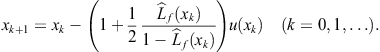 (2.136)
The following theorem was proved in Chun and Ham (2008a).
Theorem 2.8
Let ![]() be a simple zero of a sufficiently differentiable function
be a simple zero of a sufficiently differentiable function ![]() on an open interval
on an open interval ![]() and let h be any function satisfying
and let h be any function satisfying ![]() and
and ![]() . If
. If ![]() is sufficiently close to
is sufficiently close to ![]() , then the family of two-point methods defined by (2.136) has order four, and its error relation is given by
, then the family of two-point methods defined by (2.136) has order four, and its error relation is given by
![]() (2.137)
(2.137)
Several choices of the function h have been considered in Chun and Ham (2008a), for example ![]() and
and ![]() , but the choice
, but the choice ![]() is both the simplest and cheapest from the computational point of view. This value of h gives the predictor
is both the simplest and cheapest from the computational point of view. This value of h gives the predictor ![]() of Jarratt’s methods (2.123) and (2.130).
of Jarratt’s methods (2.123) and (2.130).
A similar approach has been applied in Kou et al. (2007b) for constructing the following multi-parametric family of two-point methods
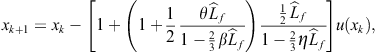 (2.138)
where ![]() is defined by (2.135) and the predictor
is defined by (2.135) and the predictor ![]() is calculated by
is calculated by
![]() (2.139)
(2.139)
It is obvious that the choice ![]() reduces (2.138) to the previous family (2.136).
reduces (2.138) to the previous family (2.136).
It was proved in Kou et al. (2007b) that the family (2.138) has order four if ![]() . Then the iterative formula (2.138) becomes (after short rearrangement)
. Then the iterative formula (2.138) becomes (after short rearrangement)
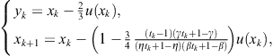 (2.140)
where
![]()
Although the iterative formula (2.140) is more complicated than (2.136), it gives some interesting special cases. For example, taking ![]() in (2.140), a particular method (2.124) from Jarratt’s family (2.123) is obtained, written in somewhat different form,
in (2.140), a particular method (2.124) from Jarratt’s family (2.123) is obtained, written in somewhat different form,
![]()
Other two-point methods based on Jarratt’s step (2.139) and the approximation (2.134) of the second derivative ![]() were developed by Kou (2007). The third-order Euler-Cauchy method
were developed by Kou (2007). The third-order Euler-Cauchy method
![]() (2.141)
(2.141)
has served as the basic method, where ![]() is defined as above. Taking
is defined as above. Taking
![]()
from (2.135) there follows
![]() (2.142)
(2.142)
Replacing this approximation into (2.141), Kou derived the following two-point method of fourth order
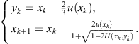 (2.143)
Using Taylor’s expansion and (2.142), in the same paper (Kou, 2007) Kou proposed the following root-free methods of fourth order:
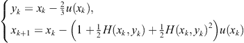 (2.144)
and
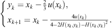 (2.145)
Note that the Euler-Cauchy method (2.141) (a special case of Hansen-Patrick’s method (1.25)) was also applied in Sharma et al. (2009) for the construction of the two-point method of fourth order
 (2.146)
where ![]() .
.
Jarratt’s step (2.139) was applied in Basu’s paper (Basu, 2008) for constructing two methods of optimal fourth order:
(I) Starting from Traub’s method (2.16), Basu obtained the two-point method
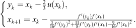 (2.147)
(II) The second two-point method
 (2.148)
was constructed using Traub’s method (2.14). Note that (2.148) is equivalent to Jarratt’s method (2.124).
2.6.2 Jarratt-like family of two-point methods
Now we will construct a family of Jarratt’s type of two-point methods which, among others, includes the methods (2.147) and (2.148). Let
![]()
Consider a two-point method in the form
![]() (2.149)
(2.149)
where ![]() is a weight function to be determined such that the method (2.149) has fourth order. As in Section 2.3, we approximate the weight function
is a weight function to be determined such that the method (2.149) has fourth order. As in Section 2.3, we approximate the weight function ![]() by its Taylor’s polynomial of third degree
by its Taylor’s polynomial of third degree

We use the Taylor expansion about the point ![]() since
since
![]()
Using symbolic computation we find the error relation of (2.149)
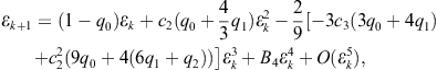
where the expression of ![]() is rather lengthy and will be given explicitly after its simplification. Hence, the two-point method (2.149) will be of order four if the coefficients of
is rather lengthy and will be given explicitly after its simplification. Hence, the two-point method (2.149) will be of order four if the coefficients of ![]() , and
, and ![]() all vanish. These conditions are satisfied if we take the weight function
all vanish. These conditions are satisfied if we take the weight function ![]() in (2.149) with the properties
in (2.149) with the properties
 (2.150)
The above error relation now becomes
![]() (2.151)
(2.151)
According to (2.150) and (2.151) we can state the following theorem.
Theorem 2.9
Let ![]() be a sufficiently differentiable function having a simple zero
be a sufficiently differentiable function having a simple zero ![]() in an open interval
in an open interval ![]() . If
. If ![]() is close enough to
is close enough to ![]() and the conditions (2.150) hold, then the family (2.149) is of order four.
and the conditions (2.150) hold, then the family (2.149) is of order four.
A number of Jarratt-like methods can be constructed for various choices of ![]() . A rather general two-parameter family is obtained using the rational function
. A rather general two-parameter family is obtained using the rational function
![]() (2.152)
(2.152)
For example, taking ![]() in (2.149), we obtain Jarratt’s method (2.148) (rediscovered by Basu (2008)). Note that Basu’s method (2.147) is obtained from (2.149) for
in (2.149), we obtain Jarratt’s method (2.148) (rediscovered by Basu (2008)). Note that Basu’s method (2.147) is obtained from (2.149) for ![]() . Here are two other examples arising from (2.152):
. Here are two other examples arising from (2.152):
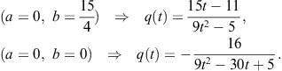
More generally, choosing
![]()
(for ![]() in (2.152),
in (2.152), ![]() ), the Jarratt family (2.123) follows from (2.149).
), the Jarratt family (2.123) follows from (2.149).
Using a different approach, Chun et al. (2012) derived a generalized family of Jarratt’s type, which is essentially the same to (2.149) and has the form
![]() (2.153)
(2.153)
where
![]()
It was shown in Chun et al. (2012) that the family (2.153) is of order four if
![]()
It is easy to show that these conditions are equivalent to (2.150) since ![]() .
.
A lot of new and old methods of Jarratt’s type can be generated from (2.153). For example, taking
![]()
in (2.153), where ![]() , we obtain (2.140).
, we obtain (2.140).
Remark 2.16
Observe that most multipoint methods considered in this book do not use more than one derivative evaluation. On the other hand, the methods presented in this section use two evaluations of the derivative, which is computationally attractive in problems where the evaluation of ![]() is rapid compared to
is rapid compared to ![]() . As noted by Jarratt (1966), such cases arise when f is defined by an integral.
. As noted by Jarratt (1966), such cases arise when f is defined by an integral.
2.7 Two-point methods for multiple roots
In Section 1.6 we gave a short review of one-point iterative methods for finding multiple zeros of a given real function f with a known order of multiplicity m. Those formulae can also be applied for finding an isolated complex zero. The presented formulae of third order depend on ![]() , and
, and ![]() . Studying one-point methods, authors have concentrated mainly on the construction of (i) new methods of third order with the known multiplicity m, see, e.g., Chun et al. (2009), Chun and Neta (2009a), and Osada (1994), or (ii) new methods with the unknown multiplicity, for instance, King (1977), Parida and Gupta (2008), Wu and Fu (2001), Wu et al. (2001), and Yun (2009, 2010, 2011).
. Studying one-point methods, authors have concentrated mainly on the construction of (i) new methods of third order with the known multiplicity m, see, e.g., Chun et al. (2009), Chun and Neta (2009a), and Osada (1994), or (ii) new methods with the unknown multiplicity, for instance, King (1977), Parida and Gupta (2008), Wu and Fu (2001), Wu et al. (2001), and Yun (2009, 2010, 2011).
Since the main goal of this book is to investigate multipoint methods, in what follows we will consider only two-point methods for finding multiple zeros of known multiplicities. The basic idea in almost all methods relies on the elimination of the second derivative. At present, n-point methods (![]() ) for multiple zeros are not of interest because of their low-computational efficiency.
) for multiple zeros are not of interest because of their low-computational efficiency.
2.7.1 Non-optimal two-point methods for multiple zeros
We start with a review of non-optimal two-point methods for multiple zeros. Using two evaluations of f and one evaluation of ![]() , Dong (1982) has constructed two methods of third order,
, Dong (1982) has constructed two methods of third order,

and
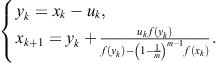 (2.154)
Employing the same information, Victory and Neta (1983) have stated the following third-order method
 (2.155)
where
![]()
By a composition of the third-order methods (2.154) and (2.155), Chun et al. (2009) have developed a one-parameter two-point method of third order,
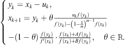
This method also requires three F.E.
A one-parameter family of third order for multiple zeros,
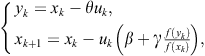 (2.156)
has been given by Neta (2008), where
![]()
As in the case of the previous methods, the family (2.156) also uses two evaluations of f and one evaluation of ![]() per iteration.
per iteration.
Two other two-point methods of third order have been developed in Dong (1987) requiring one evaluation of f and two evaluations of ![]() ,
,
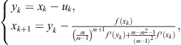
and

Homeier (2009) has proposed the following third-order method
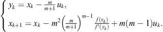
Li et al. (2009a) have constructed two families of third order methods, the first of which is given by
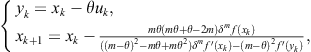
where ![]() and
and ![]() is a real parameter. The second family is defined by
is a real parameter. The second family is defined by
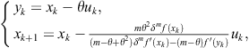
where ![]() .
.
Neta and Johnson (2008) have proposed a two-point method of fourth order requiring one function and three derivative evaluations per iteration. This method is based on the Jarratt method (Jarratt, 1966) and given by the iterative formula
![]()
where
![]() (2.157)
(2.157)
A table of values of the parameters ![]() is given in Neta and Johnson (2008) for several values of m.
is given in Neta and Johnson (2008) for several values of m.
Another fourth-order method, which also uses one function and three derivative evaluations per iteration, has been given by Neta (2010). This method is based on Murakami’s method (Murakami, 1978) and reads
![]()
where ![]() , and
, and ![]() are given by (2.157) and
are given by (2.157) and
![]()
A table of values of the parameters ![]() is given in Neta (2010) for several values of m. Li et al. (2010) got closed form formulae for several methods based on the work in Neta (2010) and Neta and Johnson (2008).
is given in Neta (2010) for several values of m. Li et al. (2010) got closed form formulae for several methods based on the work in Neta (2010) and Neta and Johnson (2008).
The presented list does not exhaust all two-point non-optimal methods for multiple zeros. However, our primary goal is to present two-point methods of optimal order four for multiple zeros, which is the topic discussed in what follows.
2.7.2 Optimal two-point methods for multiple zeros
The first optimal two-point method for multiple zeros was developed by Li et al. (2009b). Surprisingly enough, it happened almost one half of century after constructing the first optimal two-point method for simple zeros (Ostrowski, 1960). They have started with the iterative scheme of Jarratt’s type
 (2.158)
where ![]() , and
, and ![]() are parameters to be determined so that the method (2.158) has fourth order. Setting
are parameters to be determined so that the method (2.158) has fourth order. Setting ![]() , and
, and ![]() in (2.158), one gets the fourth-order Jarratt method (2.124) proposed in Jarratt (1966) (for simple zeros).
in (2.158), one gets the fourth-order Jarratt method (2.124) proposed in Jarratt (1966) (for simple zeros).
The determination of the parameters ![]() can be carried out using Taylor’s series with the help of symbolic computation by using computer algebra system such as Mathematica or Maple. Complete procedure is given in Li et al. (2009b) and we present only a part of that presentation.
can be carried out using Taylor’s series with the help of symbolic computation by using computer algebra system such as Mathematica or Maple. Complete procedure is given in Li et al. (2009b) and we present only a part of that presentation.
Let ![]() be a zero of f with multiplicity m and let
be a zero of f with multiplicity m and let
![]()
Using Taylor’s series of ![]() , and
, and ![]() about the zero
about the zero ![]() of f, the following error relation is obtained from (2.158)
of f, the following error relation is obtained from (2.158)
![]() (2.159)
(2.159)
where
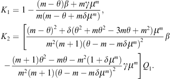
The expressions of ![]() and
and ![]() are very lengthy and will be listed after some simplification performed by a suitable choice of
are very lengthy and will be listed after some simplification performed by a suitable choice of ![]() and
and ![]() .
.
To annihilate ![]() and
and ![]() it is necessary to take
it is necessary to take
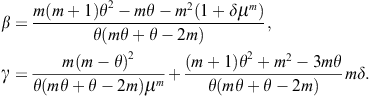
![]() (2.160)
(2.160)
where
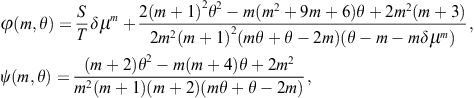
with the abbreviations

(see Li et al., 2009b).
To obtain fourth order it is necessary that ![]() and
and ![]() in (2.160) vanish. From the relations
in (2.160) vanish. From the relations ![]() and
and ![]() we obtain
we obtain
![]() (2.161)
(2.161)
Substituting ![]() and
and ![]() into the expressions for
into the expressions for ![]() and
and ![]() we get
we get
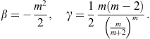 (2.162)
Returning to the iterative scheme (2.158) with the values given by (2.161) and (2.162) we obtain the following fourth order method
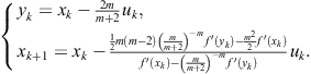 (2.163)
Since the coefficients ![]() , and
, and ![]() are annihilated, from (2.159) we obtain the error relation
are annihilated, from (2.159) we obtain the error relation
![]()
where
![]()
The two-point method (2.163) has order four and requires three F.E. per iteration. Therefore, it is optimal in the sense of the Kung-Traub conjecture. Its efficiency index is ![]() , higher than the efficiency index of any iterative (one-point or multi-point) method for multiple zeros constructed before this method.
, higher than the efficiency index of any iterative (one-point or multi-point) method for multiple zeros constructed before this method.
Li et al. (2010) derived later the iterative method (2.163) as a special case. It was done in a different way starting from the iterative scheme

Taking ![]() (that is,
(that is, ![]() ), the following two-point fourth-order method is obtained
), the following two-point fourth-order method is obtained
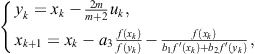 (2.164)
where

In a special case when ![]() , the iterative method (2.164) reduces to Li-Liao-Cheng’s method (2.163).
, the iterative method (2.164) reduces to Li-Liao-Cheng’s method (2.163).
Zhou et al. (2011) have generalized the two-point method (2.163) beginning from the two-point scheme
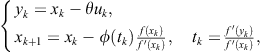 (2.165)
where ![]() is a real parameter and
is a real parameter and ![]() is at least twice differentiable. The parameter
is at least twice differentiable. The parameter ![]() and the function
and the function ![]() have to be determined so that the two-point method (2.165) reaches fourth order. This task is considered in the following theorem proved in Zhou et al. (2011).
have to be determined so that the two-point method (2.165) reaches fourth order. This task is considered in the following theorem proved in Zhou et al. (2011).
Theorem 2.10
Let ![]() be a multiple zero of multiplicity m of a function
be a multiple zero of multiplicity m of a function ![]() for an open interval
for an open interval ![]() . If an initial approximation
. If an initial approximation ![]() is sufficiently close to
is sufficiently close to ![]() , then the order of convergence of the method (2.165) is at least four when the following conditions are satisfied:
, then the order of convergence of the method (2.165) is at least four when the following conditions are satisfied:
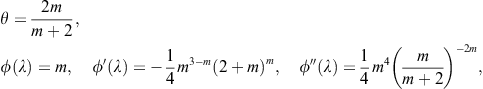
where ![]() .
.
Several special cases of the function ![]() are given in Zhou et al. (2011):
are given in Zhou et al. (2011):
To develop an iterative two-point method of optimal order four for finding multiple zeros, Sharma and Sharma (2010a) have utilized Jarratt’s multipoint iterative scheme for simple zeros (Jarratt, 1969)
![]() (2.166)
(2.166)
where
![]()
Taking ![]() , the fourth-order method (2.130) of Jarratt is obtained. The following theorem proved in Sharma and Sharma (2010a) shows that a suitable choice of parameters in (2.166) can lead to a fourth-order method for multiple zeros.
, the fourth-order method (2.130) of Jarratt is obtained. The following theorem proved in Sharma and Sharma (2010a) shows that a suitable choice of parameters in (2.166) can lead to a fourth-order method for multiple zeros.
Theorem 2.11
Let ![]() be a multiple zero of multiplicity m of a sufficiently differentiable function
be a multiple zero of multiplicity m of a sufficiently differentiable function ![]() for an open interval
for an open interval ![]() . If
. If ![]() is close enough to
is close enough to ![]() , then the iterative method (2.166) is of order four if
, then the iterative method (2.166) is of order four if

Remark 2.17
The family of two-point methods (2.165) contains as special cases Li-Liao-Cheng’s fourth-order method (2.163) (variant 3) and Sharma-Sharma’s fourth-order method (2.166) (variant 4).
We do not give numerical examples for two-point methods for multiple zeros since, having in mind Remark 2.17 and special cases of (2.165), there are no other methods for comparison.
References
1. Amat S, Busquier S, Plaza S. Review of some iterative root-finding methods from a dynamical point of view. Sci Ser A Math Sci (N.S.). 2004;10:3–35.
2. Basu D. From third to fourth order variant of Newton’s method for simple roots. Appl Math Comput. 2008;202:886–892.
3. Chun C. A family of composite fourth-order iterative methods for solving nonlinear equations. Appl Math Comput. 2007a;187:951–956.
4. Chun C. On the construction of iterative methods with at least cubic convergence. Appl Math Comput. 2007b;189(1384–1392):b0025.
5. Chun C. Some variants of King’s fourth-order family of methods for nonlinear equations. Appl Math Comput. 2007c;190:57–62.
6. Chun C. Some variants of Chebyshev-Halley methods free from second derivative. Appl Math Comput. 2007e;191:193–198.
7. Chun C. Some fourth-order iterative methods for solving nonlinear equations. Appl Math Comput. 2008;195:454–459.
8. Chun C, Ham Y. A one-parameter fourth-order family of iterative methods for nonlinear equations. Appl Math Comput. 2007a;189:610–614.
9. Chun C, Ham Y. Some fourth-order modifications of Newton’s method. Appl Math Comput. 2008b;197:654–658.
10. Chun C, Ham Y. Some second-derivative-free variants of super-Halley method with fourth-order convergence. Appl Math Comput. 2008a;195:537–541.
11. Chun C, Kim YI. Several new third-order iterative methods for solving nonlinear equations. Acta Appl Math. 2010;109:1053–1063.
12. Chun C, Neta B. A third-order modification of Newton’s method for multiple roots. Appl Math Comput. 2009a;211:474–479.
13. Chun C, Neta B. Certain improvements of Newton’s method with fourth-order convergence. Appl Math Comput. 2009b;215:821–828.
14. Chun C, Bae HJ, Neta B. New families of nonlinear third-order solvers for finding multiple roots. Comput Math Appl. 2009;57:1574–1582.
15. Chun C, Lee MY, Neta B, Džunić J. On optimal fourth-order iterative methods free from second derivative and their dynamics. Appl Math Comput. 2012;218:6427–6438.
16. Cordero A, Torregrosa JR. A class of Steffensen type methods with optimal order of convergence. Appl Math Comput. 2011;217:7653–7659.
17. Cordero A, Hueso JL, Martı´nez E, Torregrosa JR. New modifications of Potra-Pták’s method with optimal fourth and eighth orders of convergence. J Comput Appl Math. 2010;234:2969–2976.
18. Dong C. A basic theorem of constructing an iterative formula of the higher order for computing multiple roots of an equation. Math Numer Sinica. 1982;11:445–450.
19. Dong C. A family of multipoint iterative functions for finding multiple roots of equations. Int J Comput Math. 1987;21:363–367.
20. Frontini M, Sormani E. Some variant of Newton’s method with third-order convergence. Appl Math Comput. 2003;140:419–426.
21. Hansen E, Patrick M. A family of root finding methods. Numer Math. 1977;27(257–269):b0110.
22. Homeier HHH. A modified Newton method for rootfinding with cubic convergence. J Comput Appl Math. 2003;157:227–230.
23. Homeier HHH. On Newton-type methods with cubic convergence. J Comput Appl Math. 2005;176:425–432.
24. Homeier HHH. On Newton-type methods for multiple roots with cubic convergence. J Comput Appl Math. 2009;231:249–254.
25. Jarratt P. Some fourth order multipoint methods for solving equations. Math Comp. 1966;20:434–437.
26. Jarratt P. Some efficient fourth-order multipoint methods for solving equations. BIT. 1969;9:119–124.
27. King RF. A family of fourth order methods for nonlinear equations. SIAM J Numer Anal. 1973a;10:876–879.
28. King RF. A secant method for multiple roots. BIT. 1977;17:321–328.
29. Kou J. Fourth-order variants of Cauchy’s method for solving nonlinear equations. Appl Math Comput. 2007;192:113–119.
30. Kou J, Li Y, Wang X. A composite fourth-order iterative method for solving nonlinear equations. Appl Math Comput. 2007a;184:471–475.
31. Kou J, Li Y, Wang X. Fourth-order iterative methods free from second derivative. Appl Math Comput. 2007b;184:880–885.
32. Kou J, Li Y, Wang X. A family of fourth-order methods for solving nonlinear equations. Appl Math Comput. 2007c;188:1031–1036.
33. Kung HT, Traub JF. Optimal order of one-point and multipoint iteration. J ACM. 1974;21:643–651.
34. Li S, Liao X, Cheng L. A new fourth-order iterative method for finding multiple roots of nonlinear equations. Appl Math Comput. 2009a;215:1288–1292.
35. Li S, Li H, Cheng L. Some second-derivative-free variants of Halley’s method for multiple roots. Appl Math Comput. 2009b;215:2192–2198.
36. Li S, Cheng L, Neta B. Some fourth-order nonlinear solvers with closed formulae for multiple roots. Comput Math Appl. 2010;59:126–135.
37. Liu Z, Zheng Q, Zhao P. A variant of Steffensen’s method of fourth-order convergence and its applications. Appl Math Comput. 2010;216:1978–1983.
38. Maheshwari AK. A fourth-order iterative method for solving nonlinear equations. Appl Math Comput. 2009;211(383–391):b0195.
39. Kanwar V. Mamta, Kukreja VK, Singh S. On a class of quadratically convergent iteration formulae. Appl Math Comput. 2005;166:633–637.
40. Murakami T. Some fifth order multipoint iterative formulae for solving equations. J Inform Process. 1978;1:138–139.
41. Neta B. New third order nonlinear solvers for multiple roots. Appl Math Comput. 2008;202:162–170.
42. Neta B. Extension of Murakami’s high order nonlinear solver to multiple roots. Int J Comput Math. 2010;87:1023–1031.
43. Neta B, Johnson AN. High-order nonlinear solver for multiple roots. Comput Math Appl. 2008;55:2012–2017.
44. Osada N. An optimal multiple root-finding method of order three. J Comput Appl Math. 1994;51:131–133.
45. Ostrowski AM. Solution of Equations and Systems of Equations. New York: Academic Press; 1960.
46. Ostrowski AM. Solution of Equations and Systems of Equations. New York: Academic Press; 2004.
47. Özban AY. Some new variants of Newton’s method. Appl Math Lett. 2004;17:677–682.
48. Parida PK, Gupta DK. An improved method for finding multiple root and it’s multiplicity of nonlinear equations in R. Appl Math Comput. 2008;202:498–503.
49. Peng Y, Feng H, Li Q, Zhang X. A fourth-order derivative-free algorithm for nonlinear equations. J Comput Appl Math. 2011;235:2551–2559.
50. Petković LD, Petković MS. A note on some recent methods for solving nonlinear equations. Appl Math Comput. 2007;185:368–374.
51. Petković MS, Petković LD. A one parameter square root family of two-step root-finders. Appl Math Comput. 2007c;188:339–344.
52. Petković MS, Petković LD. Families of optimal multipoint methods for solving nonlinear equations: a survey. Appl Anal Discrete Math. 2010;4:1–22.
53. Petković MS, Triv cković S, Herceg Ð. On Euler-like methods for the simultaneous approximation of polynomial zeros. Japan J Idustr Appl Math. 1998;15:295–315.
54. Petković MS, Ilić S, Džunić J. Derivative free two-point methods with and without memory for solving nonlinear equations. Appl Math Comput. 2010a;217:1887–1895.
55. Potra FA, Pták V. Nondiscrete Induction and Iterative Processes. Research Notes in Mathematics vol 103 Boston: Pitman; 1984.
56. Ren H, Wu Q, Bi W. A class of two-step Steffensen type methods with fourth-order convergence. Appl Math Comput. 2009;209:206–210.
57. Salehov GS. On the convergence of the process of tangent hyperbolas. Dokl Akad Nauk SSSR. 1952;82:525–528 (in Russian).
58. Sharma JR. A composite third order Newton-Steffensen method for solving nonlinear equations. Appl Math Comput. 2005;169:242–246.
59. Sharma JR, Goyal RK. Fourth-order derivative-free methods for solving nonlinear equations. Int J Comput Math. 2006;83:101–106.
60. Sharma JR, Guha RK. Second-derivative free methods of third and fourth order for solving nonlinear equations. Int J Comput Math. 2011;88:163–170.
61. Sharma JR, Sharma R. Modified Jarratt method for computing multiple roots. Appl Math Comput. 2010a;217:878–881.
62. Sharma JR, Guha RK, Sharma R. Some variants of Hansen-Patrick method with third and fourth order convergence. Appl Math Comput. 2009;214:171–177.
63. Steffensen IF. Remarks on iteration Skand Aktuarietidskr. 1933;16:64–72.
64. Thukral R, Petković MS. Family of three-point methods of optimal order for solving nonlinear equations. J Comput Appl Math. 2010;233:2278–2284.
65. Traub JF. Iterative Methods for the Solution of Equations. Englewood Cliffs, New Jersey: Prentice-Hall; 1964.
66. Varona L. Graphic and numerical comparison between iterative methods. Math Intelligencer. 2002;24:37–46.
67. Victory HD, Neta B. A higher order method for multiple zeros of nonlinear functions. Int J Comput Math. 1983;12:329–335.
68. Weerakoon S, Fernando TGI. A variant of Newton’s method with accelerated third-order convergence. Appl Math Lett. 2000;13:87–93.
69. Wu XY, Fu DS. New higher-order convergence iteration methods without employing derivatives for solving nonlinear equations. Comput Math Appl. 2001;41:489–495.
70. Wu XY, Xia JL, Shao R. Quadratically convergent multiple roots finding method without derivatives. Comput Math Appl. 2001;42:115–119.
71. Yun BI. A non-iterative method for solving nonlinear equations. Appl Math Comput. 2008;198:691–699.
72. Yun BI. A derivative free iterative method for finding multiple roots of nonlinear equations. Appl Math Lett. 2009;22(1859–1863):b0360.
73. Yun BI. New higher order methods for solving nonlinear equations with multiple roots. J Comput Appl Math. 2011;235:1553–1555.
74. Yun BI, Petković MS. Iterative methods based on the signum function approach for solving nonlinear equations. Numer Algorithms. 2009;52:649–662.
75. Zhou X, Chen X, Song Y. Construction of higher order methods for multiple roots of nonlinear equations. J Comput Appl Math. 2011;235:4199–4206.