Chapter 7

Autodesk Maya Shading and Texturing

Shading is the term for applying colors and textures to create materials, also known in the Autodesk® Maya® software as shaders. A shader defines an object’s look—its color, tactile texture, transparency, luminescence, glow, and so forth.

Learning Outcomes: In this chapter, you will be able to
  • Differentiate between different shader types
  • Create and edit shader networks in the Hypershade window
  • Apply shaders and textures to a model
  • Set up UVs on a model for the best texture placement
  • Understand the steps to set up texture images to fit a model’s UV layout
  • Tweak UVs to align texture details

Maya Shading

When you create any objects, Maya assigns a default shader to them called Lambert1, which has a neutral gray color. The shader allows your objects to render and display properly. If no shader is attached to a surface, an object can’t be seen when rendered. In the Maya view panels, it will appear wireframe all the time, even in Shaded view.

Shading is the proper term for applying a renderable color, surface bumps, transparency, reflection, shine, or similar attributes to an object in Maya. It’s closely related to, but distinct from, texturing, which is what you do when you apply a map or other node to an attributeof a shader to create some sort of surface detail. For example, adding a scanned photo of a brick wall to the Color attribute of a shader is considered applying texture. Adding another scanned photo of the bumps and contours of the same brick wall to the Bump Mapping attribute is also considered applying a texture. Nevertheless, because textures are often applied to shaders, the entire process of shading is sometimes informally referred to as texturing. Applying textures to shaders is also called texture mapping or simply mapping. You map a texture to the color node of a shader that is assigned or applied to a Maya object.

Shaders are based on nodes. Each node holds the attributes that define the shader. You create shader networks of interconnected shading nodes, akin to the hierarchies and groups of models. These networks can be simple, or they can be intricate and involved, like when several render nodes are used to create complex shading effects.

Each shader, also known as a shading group, comprises a set of material nodes. Material nodes are the Maya nodes that hold all the pertinent rendering information about the object to which they’re assigned, such as their color, opacity, or shininess. The shading groups are the nodes that allow the connection between the surface and the material you’ve created. When you edit the shader through the Attribute Editor, as you’ll do later in this chapter, you edit its material node.

As you learn about shading in this chapter, you’ll deal at length with the Hypershade window. See Chapter 2, “Jumping in Headfirst, with Both Feet,” and Chapter 3, “The Autodesk Maya 2014 Interface,” for the layout of this window and for a hands-on introduction. You can access the Hypershade window by choosing Window ⇒ Rendering Editors ⇒ Hypershade. Shading in Maya is almost always done hand in hand with lighting. At the very least, textures are tweaked and edited in the lighting stage of production.

Shader Types

Open the Hypershade window by choosing Window ⇒ Rendering Editors ⇒ Hypershade. In the left column of the Hypershade window, you’ll see a listing of Maya shading nodes (Figure 7-1). The first section displays surface nodes, a.k.a. material nodes or shader types. Of these shader types, five are common to other animation packages as well. You’ll use two of these later in this chapter.

Figure 7-1: The Maya shading nodes

c07f001.tif

To understand a bit more about shaders, consider what makes objects appear as they do in the real world. The short answer is light. The way light bounces off an object defines how you see that object. The surface of the object may have pigments that affect the wavelength of light that reflects off it, giving the surface color. Other features of that object’s surface also dictate how light is reflected.

For the most part, shader types address the differences in how light bounces off surfaces. Most light, after it hits a surface, diffuses across an area of that surface. It may also reflect a hot spot called a specular highlight. The shaders in Maya differ in how they deal with specular and diffuse parameters according to the specific math that drives them. As you learn about the shader types, think of the things around you and what shader type would best fit them. Some Maya shaders are specific to creating special effects, such as the Hair Tube shader and the Use Background shader. It’s important to learn the fundamentals first, so I’ll cover the shading types you’ll be using right off the bat.

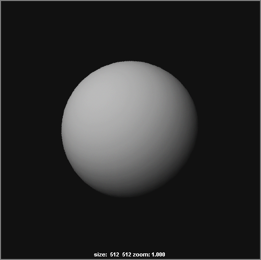
The Lambert Shader Type

The most common shader type is Lambert, an evenly diffused shading type found in dull or matte surfaces. A sheet of paper, for example, is a Lambert surface.

A Lambert surface diffuses and scatters light evenly across its surface in all directions, as you can see in Figure 7-2.

Figure 7-2: A Lambert shader

c07f002.tif

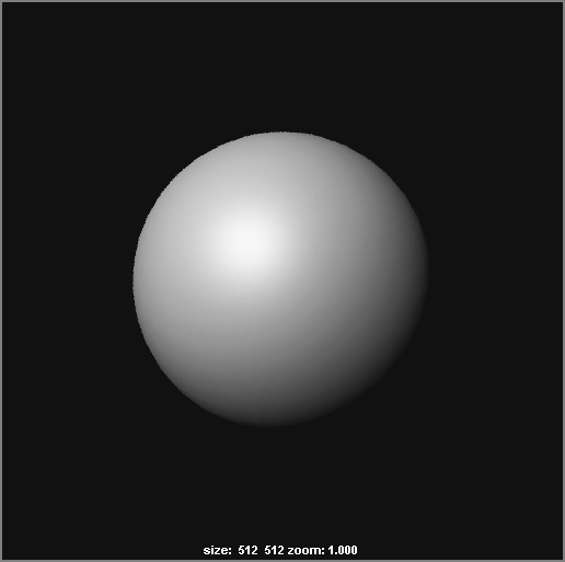
The Phong Shader Type

Phong shading brings to a surface’s rendering the notions of specular highlight and reflectivity. A Phong surface reflects light with a sharp hot spot, creating a specular highlight that drops off sharply, as shown in Figure 7-3. You’ll find that glossy objects such as plastics, glass, and most metals take well to Phong shading.

Figure 7-3: A Phong shader

c07f003.tif

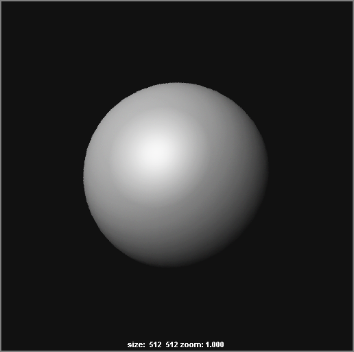
The Blinn Shader Type

The Blinn shading method brings to the surface a highly accurate specular lighting model that offers superior control over the specular’s appearance (see Figure 7-4). A Blinn surface reflects light with a hot spot, creating a specular that diffuses somewhat more gradually than a Phong. The result is a shader that is good for use on shiny surfaces and metallic surfaces.

Figure 7-4: A Blinn shader

c07f004.tif

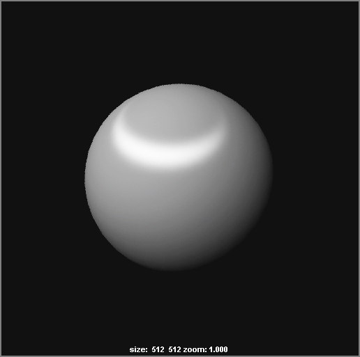
The Phong E Shader Type

The Phong E shader type expands the Phong shading model to include more control over the specular highlight. A Phong E surface reflects light much like a regular Phong does, but it has more detailed control over the specular settings to adjust the glossiness of the surface (see Figure 7-5). This creates a surface with a specular that drops off more gradually and yet remains sharper than a Blinn. Phong E also has greater color control over the specular than do Phong and Blinn, giving you more options for metallic reflections.

Figure 7-5: A Phong E shader

c07f005.tif

The Anisotropic Shader Type

The Anisotropic shader is good to use on surfaces that are deformed, such as a foil wrapper or warped plastic (see Figure 7-6).

Figure 7-6: An Anisotropic shader

c07f006.tif

Anisotropic refers to something whose properties differ according to direction. An anisotropic surface reflects light unevenly and creates an irregular-shaped specular highlight that is good for representing surfaces with directional grooves, like CDs. This creates a specular highlight that is uneven across the surface, changing according to the direction you specify on the surface. This is different than the Blinn and Phong shader types where the specular highlight is evenly distributed to make a circular highlight on the surface.

The Layered Shader Type

A Layered shader allows the stacking of shaders to create complex shading effects, which is useful for creating objects composed of multiple materials (see Figure 7-7). By using the Layered shader to texture different materials on different parts of the object, you can avoid using excess geometry.

Figure 7-7: A Layered shader

c07f007.tif

You control Layered shaders by using transparency maps to define which areas show which layers of the shader. You drag material nodes into the top area of the Attribute Editor and stack them from left to right, the left being the topmost layer assigned to the surface.

Layered shaders are valuable resources to control compound and complex shaders. They’re perfect for putting labels on objects or adding dirt to aged surfaces.

The Ramp Shader Type

A Ramptexture is a gradient that can be attached to almost any attribute of a shader as a texture node. Ramps can create smooth transitions between colors and can even be used to control particles. (See Chapter 12, “Autodesk Maya Dynamics and Effects,” to see how a ramp is used to control particles.) When used as a texture, a ramp can be connected to any attribute of a shader to create graduating color scales, transparency effects, increasing glow effects, and so on. You’ll use Ramp textures later in this chapter.

The Ramp shader is a self-contained shader node that automatically has several Ramp texture nodes attached to its attributes. These ramps are attached within the shader itself, so there is no need to connect external Ramp texture nodes. This makes for a simplified editing environment for the shader because all the colors and handles are accessible through the Ramp shader’s own Attribute Editor, as shown in Figure 7-8.

Figure 7-8: A Ramp shader in its Attribute Editor

c07f008.tif

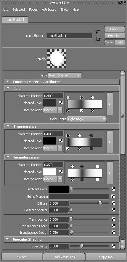
To create a new color in any of the horizontal ramps, click in the swatch to create a new ramp position. Edit its color through its Selected Color swatch. You can move the position by grabbing the circle right above the ramp and dragging left or right. To delete a color, click the box beneath it.

Ramp textures are automatically attached to the Color, Transparency, Incandescence, Specular Color, Reflectivity, and Environment attributes of a Ramp shader. In addition, a special curve ramp is attached to the Specular Roll Off attribute to allow for more precise control over how the specular highlight diminishes over the surface.

Shader Attributes

Shaders are composed of nodes just like other Maya objects. Within these nodes, attributes define what shaders do. Here is a brief rundown of the common shader attributes with which you’ll be working:

Color An RGB or HSV value defines what color the shader is when it receives a neutral color light. For more on RGB and HSV, see Chapter 1, “Introduction to Computer Graphics and 3D.”
Transparency The higher the Transparency value, the less opaque and more see-through the object becomes.
Although usually expressed in a black-to-white gradient, with black being opaque or solid and white being totally clear, transparency can have color. In a color transparency, the shader’s color shifts because only some of its RGB values are transparent, as opposed to the whole.
Ambient Color This color affects the Color attribute of the shader as more ambient light is created in the scene. Ambient color tends to flatten an object because this attribute evenly colors the object. This attribute is primarily used to create flat areas and should be used with care. The default is black, which keeps the darker areas of a surface dark. The lighter the ambient color, the lighter those areas are. A bright Ambient Color setting flattens out an object, as shown in Figure 7-9.

Figure 7-9: Ambient color values

c07f009.eps
Incandescence This attribute is the ability to self-illuminate. Objects that seem to give off or have their own light, such as an office’s fluorescent light fixture, can be given an Incandescence value. Incandescence doesn’t, however, light objects around it in regular renders, nor does it create a glow. It also serves to flatten the object into a pure color. As you’ll see in Chapter 11, “Autodesk Maya Rendering,” incandescence can also help light a scene in the mental ray® Final Gather rendering. The value of Incandescence (as well as the color) of an object is used to calculate the overall brightness in a Final Gather scene (see Figure 7-10).

Figure 7-10: Incandescence values

c07f010.eps
Bump Mapping This attribute creates a textured feel for the surface by adding highlights and shadows to the render. It doesn’t alter the surface of the geometry, although it makes the surface appear to have ridges, marks, scratches, and so forth. The bump map has to be a texture node such as a ramp, a fractal noise, or an image file. The more intense the variation in tones of that map, the greater the bump. Bump maps are frequently used to make surfaces look more real, because nothing in reality has a perfectly smooth surface. Using bumps very close up may create problems; bumps are generally good for adding inexpensive detail to a model that isn’t in extreme close-up (see Figure 7-11).

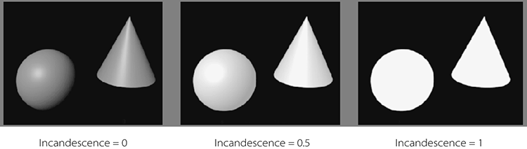
Figure 7-11: The effects of a bump map

c07f011.eps

Geometry when seen close up, where you have to change the topology of the model physically using texture maps, requires displacement maps. I’ll cover displacement maps in Chapter 11.

Diffuse This value governs how much light is reflected from the surface in all directions. When light strikes a surface, light disperses across the surface and helps illuminate it. The higher this value, the brighter its object is when lit, because more of the striking light is reflected from the surface. The lower the Diffuse value, the more light is “absorbed” into the surface, yielding a darker result, especially in areas that aren’t well lit. Metals have very low Diffuse values because they rely on reflections and direct light (see Figure 7-12).

Figure 7-12: How a Diffuse value affects a shader’s look

c07f012.eps
Translucence and Translucence Focus The Translucence and Translucence Focus attributes give the material the ability to transmit light through its surface, like a piece of canvas in front of a light. At a value of 1 for Translucence, all light shines through the object; at 0, none does. The Translucence Focus attribute specifies how much of that light is scattered. A light material such as paper should have a high translucence focus, and thicker surfaces should have low focus rates.
Glow Intensity Found in the Special Effects section of the Attribute Editor, the Glow Intensity attribute adds a glow to the object, as if it were emitting light into a foggy area (see Figure 7-13). You’ll add glow to an object in Chapter 10, “Autodesk Maya Lighting.”

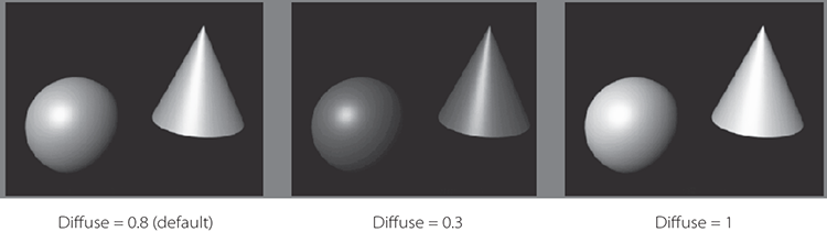
Figure 7-13: Adding a glow

c07f013.eps
Matte Opacity Objects rendered through Maya generate a solid matte. Where there is an object, the matte is white; where there is nothing, the matte is black. Mattes helps compositing programs, which bring together elements created independently into a single composite scene, to separate rendered CG from their backgrounds. Turning down the slider decreases the brightness of the object’s matte, making it appear more transparent. This technique is usually used for compositing tricks or to make an object render in RGB but not appear in any composites. For more information about mattes, see the sidebar “Image Mattes” in this chapter, and see Chapter 11.
Raytrace Options With raytracing, you can achieve true reflections and refractions in your scene. This subset of attributes allows you to set the shader’s raytracing abilities. See Chapter 11 for more on raytracing.

Some attributes are available only with certain shader types. The following are the attributes for the Phong, Phong E, and Blinn shaders:

Specular Color The color of the highlights on a shiny surface. Black produces no specular, and white creates a bright one.
Reflectivity The amount of reflection visible in the surface. The higher the value, the more reflective the object will render. Increasing this value increases the visibility of the Reflected Color attribute or of true reflections in the scene when raytraced.
Reflected Color Gives the surface a reflection. Texture maps are generally assigned to this attribute to give the object a reflection of whatever is in the image file or texture without having to generate time-consuming true reflections with a raytraced render. Using raytracing to get true reflections, however, is the only way to generate reflections of other objects in the scene.
Cosine Power Available only with a Phong shader. This attribute changes the size of the shiny highlights (a.k.a. specular) on the surface. The higher the number, the smaller the highlight looks.

Image Mattes
As you learned in Chapter 1 (and will explore further in Chapter 11), image files are stored with a red, a green, and a blue channel that keep the amount of each color in each pixel of the image. Some image formats, including TIFF and TARGA, also have an alpha channel, known as a matte channel or image matte. This is a grayscale channel that controls the opacity of an image. Completely white parts of the matte make those parts of the image opaque (solid), whereas black parts make those parts of the image fully transparent. Gray in the matte channel makes those parts of the image partly transparent. These mattes are used in compositing—bringing together elements created separately into a single composite scene. See Chapter 11 for an example of how an alpha channel works.

Roughness, Highlight Size, Whiteness Control the specular highlight on a Phong E surface only. They control specular focus, amount of specular, and highlight color, respectively.
mental ray Attributes Because Autodesk integrates features of the mental ray rendering engine into Maya, an object’s Attribute Editor usually includes a set of mental ray options. Shaders are no different. If you open the Mental Ray heading in the Attribute Editor for a shader, you’ll see attributes such as Reflection Blur and Irradiance, as well as a few ways to override the Maya shading attributes with those of mental ray.

An in-depth discussion of the mental ray attributes is beyond the scope of this introductory text. But it’s a good idea to know that this brief section is available to you after you have more experience with rendering and you want to work with mental ray at its more advanced levels in Maya. You’ll work with mental ray in Chapters 10 and 11.


The Autodesk website lists several premade shaders for your use. Maya also includes a shader library on its installation CD.

Shading and Texturing the Table Lamp

In the following section, you’ll add shaders to the table lamp from Chapter 6, “Practical Experience.” The lamp is fairly straightforward to shade. Use lampScene_v04.mb from the TableLamp project from the companion website. You have four different colors on the body of the biplane and lamp itself, a two-tone lampshade, and a metal stem. You’ll start by making shaders in the Hypershade.

1. Open the Hypershade (Window ⇒ Rendering Editors ⇒ Hypershade). You’ll notice that the shaders for the reference planes that have the pictures of the lamp are in the scene, and the names are in red (Figure 7-14). The red signifies that the shaders are part of a scene file that is referenced into the current scene. They cannot be deleted here; you will have to go into the original model scene to delete them. You’ll do that in the next step. You’ll also notice the Lambert shaders for the lamp shade reference planes used in the modeling phase.

Figure 7-14: The reference plane shaders are still here!

c07f014.tif
2. Open airplaneModel_v06.mb, and then open the Hypershade window. Since you already deleted the geometry for the reference planes, it’s easy to flush the now unused shaders for them. In the Hypershade, select Edit ⇒ Delete Unused Nodes, and they will disappear. Save the scene as airplaneModel_v07.mb.
3. Open the lampScene_v04.mb file again, and then choose File ⇒ Reference Editor. Click the airplaneModel_v06.mb entry, and choose Reference ⇒ Replace Reference. Navigate to and select airplaneModel_v07.mb that you just saved in the Scenes folder. The biplane will disappear for a second and reappear back in place. The reference plan Lambert shaders are now gone. In the Hypershade, select Edit ⇒ Delete Unused Nodes to flush the lamp shade reference Lambert shaders as well. They were not referenced.
4. Create four new Blinn shaders. Name them blue, red, green, and black. An organized Hypershade is a happy Hypershade.
5. Double-click the blue Blinn shader, and in the Attribute Editor, click the color swatch to open the Color Chooser. Set an HSV value of 234, 0.91, .390, as shown in Figure 7-15.

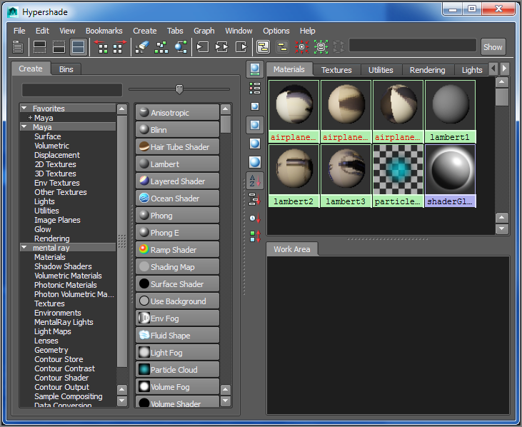
Figure 7-15: Create the blue shader.

c07f015.tif
6. Go through the other three Blinn shaders and set their HSV colors according to Table 7-1. See also Figure 7-16.

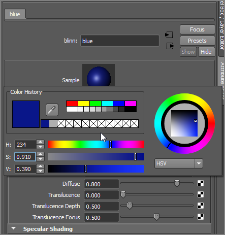
Figure 7-16: The four Blinn shaders

c07f016.tif

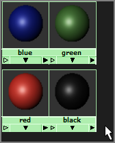
Table 7-1: HSV color values for the lamp’s colors

Table 07-01
7. Select the wings of the biplane and the base of the lamp, and assign the blue Blinn.
8. Select the propeller cap (named propCap) as shown in Figure 7-17, and assign the green Blinn.

Figure 7-17: Assign the green Blinn to the propeller cap.

c07f017.tif
9. Select the wheels, and assign them to the black Blinn.
10. Select the body of the biplane, the wheel assembly (named wheelAssembly), and its propeller blades, and assign the red Blinn (Figure 7-18). Notice in the color photos in the Color Section of this book that the lamp’s biplane body is red but has blue stabilizer wings.

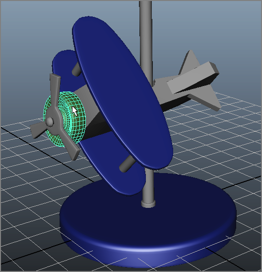
Figure 7-18: Assign the red Blinn to the biplane.

c07f018.tif
11. Select the faces that make up the stabilizer wings (as shown in Figure 7-19), and assign them to the blue Blinn.

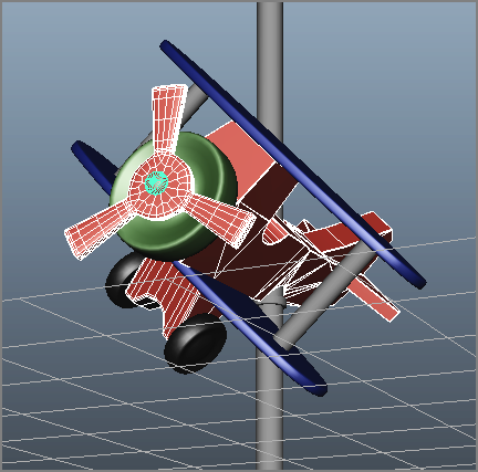
Figure 7-19: Assign blue to the faces of the back stabilizer wings.

c07f019.tif

Assigning shaders to the faces of a mesh and not the entire mesh itself works great in many cases; however, this is not a common practice in professional workflows, especially when using render layers expansively. Instead, UVs are laid out for the mesh, and different colors are assigned through maps. You will see this workflow later when you texture the wheels for a toy wagon. For your purposes just starting out, assigning to faces is a great way to explore multiple colors and materials on a single mesh.

12. Finally, select the wing support cylinders shown in Figure 7-20 and make them red as well.

Figure 7-20: Select the wing supports and make them red.

c07f020.tif

The Socket, Stem, and Lampshade

Now let’s get some shaders made for the rest of the lamp.

1. Create a new Phong shader, make it black in color like the wheel Blinn color, and call it shinyBlack. Select the light bulb socket, and assign the new black Phong to it. The Phong is just a bit shinier than the Blinn, perfect for the socket.
2. In the Hypershade, create a new Phong for the metal parts of the lamp. Give it a blue-gray color (HSV of 222, 0.15, 0.5) and a low Diffuse value of 0.15, as shown below the Color Chooser in Figure 7-21. Name the shader metal.

Figure 7-21: Create the metal’s Phong shader.

c07f021.tif
3. Select the stem and all the metal parts of the lamp shown in Figure 7-22, and assign the metal Phong shader to them. The metal parts will turn black in the view panel displays since metal is dependent on reflections for its look. You will not worry about that until a little later in this chapter and then again when you render the lamp in Chapter 11.

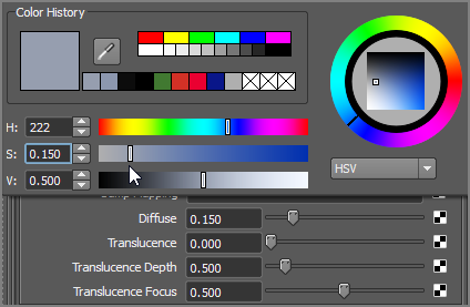
Figure 7-22: Assigning the lampshade Lambert

c07f022.tif
4. Finally, the lamp shade is a simple texture of an eggshell white color. Using a photo of the lampshade, you can create a texture swatch to use on the shade. Create a new Lambert shader, and call it lampShade.
5. Double-click the lampShade Lambert to open the Attribute Editor. Click the Map button next to the Color attribute. Select File to create a File Texture node attached to the Color attribute.
6. In the Attribute Editor, click the folder icon next to the Image Name text box, and navigate to the Sourceimages folder in the TableLamp project. Select the lampShadePatch.jpg file. Assign the Lambert to the lampshade as shown in Figure 7-22, but not the blue trim on the top and bottom. Press 6 in the persp view to enable Textured display mode.
7. Set up your render parameters so that you can render your lamp using the default lighting already in the scene while you’re tweaking shaders to get them right. Choose Window ⇒ Rendering Editors ⇒ Render Settings, or click the Render Settings icon (c07g001.tif) in the menu bar to open the Render Settings window. Make sure Render Using is set to Maya Software.
8. In the Image Size section on the Common tab, set Presets to 640×480. In the Anti-Aliasing Quality section on the Maya Software tab, use the Intermediate Quality preset. This will give you a good look for the final render with a short render time.
9. If you render a frame of the lamp, the lampshade’s texture is a bit too stretched; it needs to tile a few times. In the Hypershade, select the lampShade Lambert node, and click the Input And Output Connections icon (c07g002.tif). Click the place2dTexture1 node, as shown in Figure 7-23, and open the Attribute Editor. Set the Repeat UV values to 4 and 4 as shown.

Figure 7-23: Tile the lampshade texture.

c07f023.tif
10. Render, and the lampshade should look nicer. Now for the blue trim. In the Hypershade, select the lampShade Lambert and choose Edit ⇒ Duplicate ⇒ Shading Network to create a copy of all the shading nodes. You will use this copy to make a blue version for the trim. Name the copy lampShadeBlue, as shown in Figure 7-24.

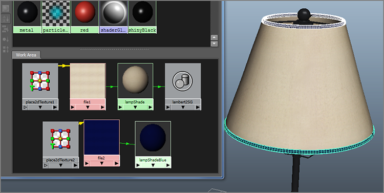
Figure 7-24: Create a copy of the lampShade Lambert.

c07f024.tif
11. Click File2, and open the Attribute Editor. Under the Color Balance heading, click Color Gain, and give it a blue color with HSV of 234, 0.91, 0.39. The eggshell white lamp shade now turns to blue in the copied shader network. Assign it to the top and bottom trim of the lamp shade, as shown in Figure 7-25.

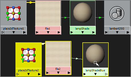
Figure 7-25: Assign the top and bottom trim to the blue-colored lampshade Lambert.

c07f025.tif
Save your work. You can compare it to the lampScene_v05.mb file at this stage.

The Metal Parts

Now let’s focus a little bit on the metal. Metal surfaces are all about reflections, as opposed to simple colors like the rest of the lamp.

1. Select the metal Phong shader. In the Attribute Editor, click the gray swatch for Specular Color. By changing this color, you control the hue and brightness of the highlights on this surface. Use a bright faded blue with HSV values of 208, 0.20, and 0.90.
2. In the Specular Shading heading, increase the spreadof the specular highlights by changing Cosine Power from the default of 20 to 2.0. Doing so creates a large area for the bright highlights, implying a polished reflective surface.
3. Rendering will still yield a black but shinier surface for the stem. You need reflections. You will explore this in detail in Chapter 11, but you will create a simple reflection “cheat” to use here by using an environment map. Select the metal Phong shader.
4. In the Attribute Editor, click the Map button next to the Reflected Color attribute, as shown in Figure 7-26. Doing so attaches a new node to create a reflection and opens the Create Render Node window.

Figure 7-26: Assigning a Reflected Color texture.

c07f026.tif
5. Click the Env Textures section, and select Env Chrome, as shown in Figure 7-27. An environment texture will provide an interesting reflection.

Figure 7-27: Select the Env Chrome texture.

c07f027.tif
6. Move the Reflectivity slider from 0.50 to 0.85. The higher this number, the more prominent the reflected color in the surface. Figure 7-28 shows the lamp before (left) and after (right) mapping a reflection. The Env Chrome reflection texture makes the metal parts of the lamp look polished by reflecting a grid representing the ground and a bright blue sky.

Figure 7-28: The lamp stem before (left) and after (right) a reflection is mapped onto the shader.

c07f028.tif

The lamp is saved as lampScene_v06.mb to catch you up to this final point.

You can embellish a model a lot at the texturing level. The more you explore and experience shaders and modeling, the better you’ll be at juggling modeling with texturing to get the most effective solution.

You’ll begin UV layout and texturing a child’s red wagon later in this chapter and then go into more detailed texturing with the decorative box, which you’ll then light and render in mental ray. For even more practice, try loading the catapult model from Chapter 4, “Beginning Polygonal Modeling,” and texturing it from top to bottom.

Textures and Surfaces

Texture nodes generate maps to connect to an attribute of a shader. There are two types of textures: procedural and bitmapped (sometimes called maps). Procedural textures use the Maya nodes attributes to generate an effect, such as ramp, checkerboard, or fractal noise textures. You can adjust each of these procedural textures by changing their attribute values.

A map, on the other hand, is a saved image file that is imported into the scene through a file texture node. These files are pregenerated through whatever imaging programs you have and include digital pictures and scanned photos. You need to place all texture nodes onto their surfaces through the shader. You can map them directly onto the surfaces’ UV values or project them.

UV Mapping

UV mapping places the texture directly on the surface and uses the surface coordinates (called UVs) for its positioning. In this case, you must do a lot of work to line up the UVs on the surface to make sure the created images line up properly. What follows is a brief summary of how UV mapping works. You’ll get hands-on experience with UV layout with the red wagon and decorative box exercises later in this chapter.

Just as 3D space is based on coordinates in XYZ, surfaces have coordinates denoted by U and V values along a 2D coordinate system for width and height. The UV value helps a texture position itself on the surface. The U and V values range from 0 to 1, with (0,0) UV being the origin point of the surface.

Maya creates UVs for primitive surfaces automatically, but frequently you need to edit UVs for proper texture placement, particularly on polygonal meshes after you’ve edited them. In some instances, placing textures on a poly mesh requires projecting the textures onto the mesh, because the poly UVs may not line up as expected after the mesh has been edited. See the next section, “Using Projections.”

If the placement of your texture or image isn’t quite right, simply use the 2D placement node of the texture node to position it properly. See the section “Texture Nodes” later in this chapter for more information.

Using Projections

You need to place textures on the surface. You can often do so using UV placement, but some textures need to be projected onto the surface. A projection is what it sounds like. The file image, ramp, or other texture being used can be beamed onto the object in several ways.

You can create any texture node as either a normal UV map or a projected texture. In the Create Render Node window, clicking a texture icon creates it as a normal mapped texture. To create the texture as a projection, you must right-click the icon and select Create As Projection (see Figure 7-29).

Figure 7-29: Selecting the type of map layout

c07f029.tif

When you create a projected texture, a new node is attached to the texture node. This projection node controls the method of projection with an attached 3D placement node, which you saw in the axe exercise. Select the projection node to set the type of projection in the Attribute Editor (see Figure 7-30).

Figure 7-30: The projection node in the Attribute Editor

c07f030.tif

Setting the projection type will allow you to project an image or a texture without having it warp and distort, depending on the model you’re mapping. For example, a planar projection on a sphere will warp the edges of the image as they stretch into infinity on the sides of the sphere.

Try This In a new scene, create a NURBS sphere and a NURBS cone, and place them side-by-side. Create a Blinn shader, and assign it to both objects. In the Blinn shader’s Attribute Editor, set its Color attribute to a checkerboard pattern, as shown in Figure 7-31.

Figure 7-31: Assign a checkerboard pattern to the sphere and cone with Normal checked.

c07f031.tif

Try removing the color map from the Blinn shader. In the Blinn shader’s Attribute Editor, right-click and hold the attribute’s title word Color, and then choose Break Connection from the context menu. Doing so severs the connection to the checker texture map node and resets the color to gray. Now, re-create a new checker texture map for the color, but this time create it as a projection by right-clicking the icon in the Create Render Node window. In the illustration on the left in Figure 7-32, you see the perspective view in Texture mode (press the 6 key) with the two objects and the planar projection placement node.

Figure 7-32: A planar projection checkerboard in the view panel (left) and rendered (right)

c07f032.tif

Try moving the planar placement object around in the scene to see how the texture maps itself to the objects. The illustration on the right of Figure 7-32 shows the rendered objects.

Try the other projection types to see how they affect the texture being mapped.

Projection placement nodes control how the projection maps its image or texture onto the surface. Using a NURBS sphere with a spherical projected checker, with U and V wrap turned off on the checkerboard texture, you can see how manipulating the place3dTexture node affects the texture.

In addition to the Move, Rotate, and Scale tools, you can use the Special Manipulator tool (press T to activate or click the Show Manipulator Tool icon in the toolbar) to adjust the placement. Figure 7-33 shows this tool for a spherical projection.

Figure 7-33: The spherical projection’s Manipulator tool

c07f033.tif

Drag the handles on the Special Manipulator to change the coverage of the projection, orientation, size, and so forth. All projection types have Special Manipulators. Figure 7-34 shows the Manipulator wrapping the checkerboard pattern in a thin band all the way around the sphere.

Figure 7-34: The Manipulator wrapping the checkerboard texture around the sphere (left, perspective view; right, rendered view).

c07f034.tif

To summarize, projection textures depend on a projector node to position the texture onto the geometry. If the object assigned to a projected texture is moving, consider grouping the projection placement node to the object itself in the Outliner.

Texture Nodes

You can create a number of texture nodes in Maya. This section covers the most important. All texture nodes, however, have common attributes that affect their final look. Open the Attribute Editor for any texture node (see Figure 7-35). The two top sections affect the color balance of the texture. The Color Balance and Effects sections are described here:

Figure 7-35: Some common attributes for all texture nodes

c07f035.tif
Color Balance This set of attributes adjusts the overall brightness and color balance of your texture. Use these attributes to tint or brighten a texture (as you did with the blue trim of the lampshade) without having to change all the individual attributes of the shader.
Effects You can invert the texture’s color space by clicking the Invert check box. This changes black to white and white to black in addition to inverting the RGB values of colors.

You can map textures to almost any shader attribute for detail. Even the tiniest amount of texture on a surface’s bump, specular, or color increases its realism.

Place2dTexture Nodes

The 2D texture nodes come with a 2D placement node that controls their repetition, rotation, size, offset, and so on. Adjust the setting in this node of your 2D texture in the Attribute Editor, as shown in Figure 7-36, to position it within the Shader network.

Figure 7-36: A 2D placement node in the Attribute Editor

c07f036.tif

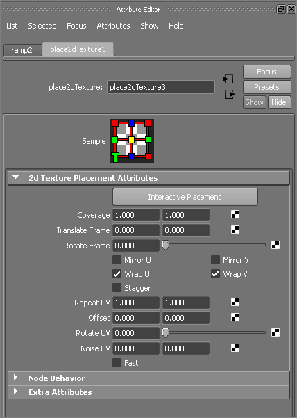
The Repeat UV setting controls how many times the texture is repeated on whatever shader attribute it’s connected to, such as Color. The higher the wrap values, the smaller the texture appears, but the more times it appears on the surface.

The Wrap U and Wrap V check boxes allow the texture to wrap around the edges of their limits to repeat. When these check boxes are turned off, the texture appears only once, and the rest of the surface is the color of the Default Color attribute found in the texture node.

The Mirror U and Mirror V settings allow the texture to mirror itself when it repeats. The Coverage, Translate Frame, and Rotate Frame settings control where the image is mapped. They’re useful for positioning a digital image or a scanned picture.
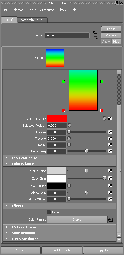
Ramp Texture

A ramp is a gradient in which one color transitions into the next color. You’ve already seen how useful a ramp can be in positioning materials in a Layered shader. It’s also perfect for making color gradients, as shown in Figure 7-37.

Figure 7-37: The Ramp texture

c07f037.tif

Use the round handles to select the color and to move it up and down the ramp. The square handle to the right deletes the color. To create a new color, click inside the ramp.


The Ramp texture is different from the Ramp shader. The Ramp shader automatically has several Ramp textures mapped to some of its attributes.

The Type setting allows you to create a gradient running along the U or V direction of the surface, as well as to make circular, radial, diagonal, and other types of gradients. The Interpolation setting controls how the colors grade from one to the next.

The U Wave and V Wave attributes let you add a squiggle to the U or V coordinate of the ramp, and the Noise and Noise Freq (frequency) attributes specify randomness for the placement of the ramp colors throughout the surface.

Using the HSV Color Noise attributes, you can specify random noise patterns of Hue, Saturation, and Value to add some interest to your texture. The HSV Color Noise options are great for making your shader just a bit different to enhance its look.

Fractal, Noise, and Mountain Textures

These textures are used to create a random noise pattern to add to an object’s Color, Transparency, or any other shader attribute. For example, when creating a surface, you’ll almost always want to add a little dirt or a few surface blemishes to the shader to make the object look less CG. These textures are commonly used for creating bump maps.

Bulge, Cloth, Checker, Grid, and Water Textures

These textures help create surface features when used on a shader’s Bump Mapping attribute. Each creates an interesting pattern to add to a surface to create tactile detail, but you can also use them to create color or specular irregularities.

When used as a texture for a bump, Grid is useful for creating the spacing between tiles, Cloth is perfect for clothing, and Checker is good for rubber grips. Placing a Water texture on a slight reflection makes for a nice poolside reflection in patio furniture.

The File Node

You use the file node to import image files into Maya for texturing. For instance, if you want to texture a CG face with a digital picture of your own face, you can use the file node to import a Maya-supported image file.

Importing an Image File as a Texture

To attach an image to the Color attribute of a Lambert shader, for example, follow these steps:

1. Create the Lambert shader. (Phong, Blinn, or any of the shaders will do.)
2. Click the Map button to map a texture on the Color attribute of the new Lambert shader. Select the file node as a normal texture. (You can also use a projected texture with an image file.) The Attribute Editor shows the attribute for the file node; see Figure 7-38.

Figure 7-38: The file texture node

c07f038.tif
3. Next to the Image Name attribute, click the Folder icon to open the file browser. Find the image file of choice on your computer. (It’s best to put images to use as textures in the project’s Sourceimages folder. As a matter of fact, the file browser defaults directly to the Sourceimages folder of your current project.) Double-click the file to load it.
4. After you import the image file, it connects to the Color attribute of that shader and also automatically connects the alpha to transparency if there is an alpha channel in the image. You can position it as you please by using its place2dTexture node or by manipulating the projection node if you created the file texture node as a projection.

You can attach an image file to any attribute of a shader that is mappable, meaning it’s able to accept a texture node. Frequently, image files are used for the color of a shader as well as for bump and transparency maps. You can replace the image file by double-clicking the file texture node in the Hypershade and choosing another image file with the file browser. Maya disconnects the current image file and connects the new file.

Using Photoshop Files: The PSD File Node

Maya can also use Adobe Photoshop PSD files as image files in creating shading networks. The advantage of using PSD files is that you can specify the layers within the Photoshop file for different attributes of the shader, as opposed to importing several image files to map onto each shader attribute separately. This, of course, requires a modest knowledge of Photoshop and some experience with Maya shading. As you learn how to shade with Maya, you’ll come to appreciate the enhancements inherent in using Photoshop networks.

Try This You’ll create a single Photoshop file that will shade this sphere with color as well as transparency and a bump. Again, you’re doing this instead of creating three different image files (such as TIFFs) for each of those shading attributes.
1. Create a NURBS sphere in a new scene, and assign a new Lambert shader to it. You can do this through the Hypershade or by choosing Lighting/Shading ⇒ Assign New Material ⇒ Lambert in the Rendering menu set. This creates a new shader and assigns it to the selection, in this case your sphere.
2. Select the sphere, and choose Texturing ⇒ Create PSD Network. In the option box that opens, select Color, Transparency, and Bump from the list of attributes on the left side, and click the right arrow to move them to the Selected Attributes list on the right, as shown in Figure 7-39.

Figure 7-39: The Create PSD Network Options window

c07f039.tif
3. Select a location and filename for the image. By default, Maya places the PSD file it generates under the Sourceimages folder of your current project, named after the surface to which it applies. Click Create.
4. In Photoshop, open the newly created PSD file. You see three layers grouped under three folders named after the shader attributes you selected when creating the PSD file. There are folders for lambert2.bump, lambert2.transparency, and lambert2.color, as well as a layer called UVSnapShot.
The UVSnapShot layer gives you a wireframe layout of the UVs on the sphere as a guideline to paint your textures. Because the sphere is an easy model, you don’t need this layer, so turn it off. You’ll use UV SnapShot later in this chapter when texturing a toy wagon.
You can now paint whatever image you want into each of the layers to create maps for each of the shader attributes, all in one convenient file. Save the PSD file. You can save over it or create a new filename for the painted file.
5. In Maya, open the Hypershade, and open the Attribute Editor for the Lambert shader assigned to the sphere (in this case, Lambert2). If you graph the connections to the Lambert shader in the Hypershade window’s work panel, you see that the PSD file you generated is already connected to the Color, Bump, and Transparency attributes of the shader, with the proper layering set for you, as shown in Figure 7-40.

Figure 7-40: The PSD network for the Lambert shader in the Hypershade shows the connections to Color, Bump, and Transparency.

c07f040.tif
6. Open the file nodes for the shader, and replace the PSD file with your new painted PSD file. If you saved your PSD file with the same name, all you need to do is click the Reload button to update the psdFile node.

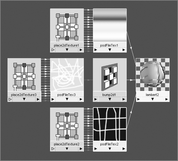
If you decide that you need to add another attribute to the PSD file’s layering or if you need to remove an attribute, you can edit the PSD network. Select the shader in the Hypershade, and choose Edit ⇒ Edit PSD Network. In the option box, select new attributes to assign to the PSD file, or remove existing attributes and their corresponding Photoshop layer groups. When you click Apply or Edit, Maya saves over the PSD file with the new layout.

3D and Environment Textures

3D textures are projected within a 3D space. These textures are great for objects that need to reflect an environment, for example.

Instead of simply applying the texture to the plane of the surface as 2D textures do, 3D textures create an area in which the shader is affected. As an object moves through a scene with a 3D placement node, its shader looks as if it swims, unless that placement node is parented or constrained to that object. (For more on constraints, see Chapter 9, “More Animation!”)

Disconnecting a Texture

Sometimes, the texture you’ve applied to an object isn’t what you want, and you need to remove it from the shader. To do so, double-click the shader in the Hypershade to open its Attribute Editor.

You can then disconnect an image file or any other texture node from the shader’s attribute by right-clicking the attribute’s name in the Attribute Editor and choosing Break Connection from the context menu, as shown in Figure 7-41.

Figure 7-41: Right-clicking a shader’s attribute allows you to disconnect a texture node from the shader.

c07f041.tif

Textures and UVs for the Red Wagon

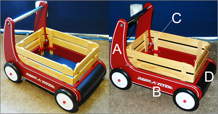
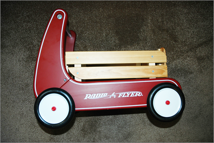
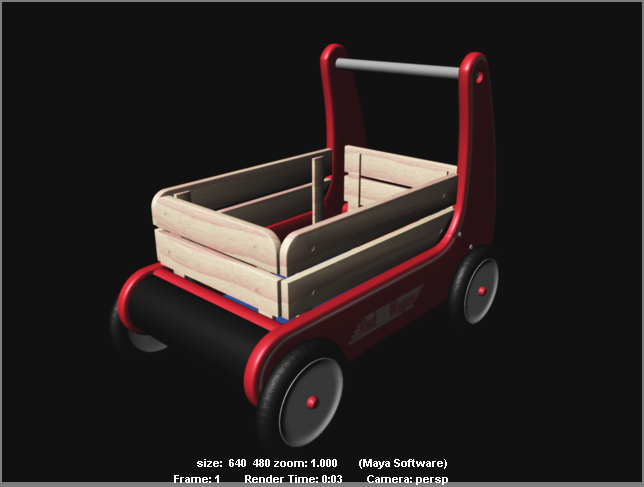
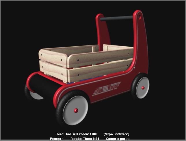
Now you’ll use a child’s red wagon toy model, to which you will assign shaders. The real wagon is shown in Figure 7-42. Take a good look at the image of the toy wagon in the Color Section of this book to see how the red wagon is colored. The wagon is fairly simple; it will need a few colored shaders (Red, Black, Blue, and White) for the body, along with a few texture maps for the decals—which is where the real fun begins. The wagon will also require some more intricate work on the shaders and textures for the wood railings and silver metal screws, bolts, and handlebar; these will be a good foray into image maps and UVs.

Figure 7-42: The red wagon and its named parts

c07f042.tif

This exercise is a prime example of how lighting and shading go hand in hand.

Assigning Shaders

Load the file RedWagonModel.ma from the Scenes folder of the RedWagon project to begin shading the model of the wagon.


Shading is the common term for adding shaders to an object.

Study the color images of the wagon, and see how light reflects off its plastic, metal, and wood surfaces. Blinn shaders will be perfect for nearly all the parts of the wagon. Follow these steps:

1. Open the Hypershade window, and create four Blinn shaders.
2. Assign the following HSV values to the Color attribute of each Blinn shader, and name them as shown in Table 7-2 and in Figure 7-43. You’ll create the Chrome Metal and Wood shaders later.

Figure 7-43: Create the four colored Blinn shaders.

c07f043.tif

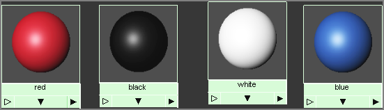
Table 7-2: HSV color values for the wagon’s colors

Table 07-02

Initial Assignments

Look at the photo of the wagon in the Color Section in the middle of this book. The bullnose and tires are black, the wheel rims are white, the floor is blue, the screws and bolts and handlebar are chrome metal, the railings are wood, and the main body is red. Assign shaders to the wagon according to the color photo and the following steps:

1. In the view panel, select the side panels (the A and B panels, without the screws and bolts) and the wheel rim caps, as shown in Figure 7-44, and assign the Red Blinn shader to them. Press 6 to enter Texture Display mode.

Figure 7-44: Assign the Red shader.

c07f044.tif
2. Select the wheelMesh objects for all four wheels, and assign them the White shader. The tires also turn white, but you’ll fix that shortly; don’t worry about it now. See Figure 7-45.

Figure 7-45: Assign the White shader.

c07f045.tif
3. Select the bullnose (the rounded cylinder in front of the wagon), and assign it the Black Blinn.
4. Select the wagonFloor object, and assign it the Red shader, as shown in Figure 7-46. You’ll notice that the front and back bodies of the wagon turn red as they’re supposed to, but so does the floor of the wagon, which should be blue according to the photo in the Color Section. If you try to assign the Blue shader to the wagon floor mesh, the floor will be correct, but the front and back body of the wagon will be blue and not red. You’ll fix this later.

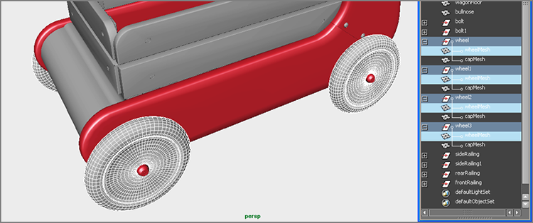
Figure 7-46: Assign the Red shader to the wagon floor just for now; you’ll change it to blue later.

c07f046.tif

Now you have initial assignments for the basic colors of the wagon’s body. Let’s tweak these shaders’ colors next.

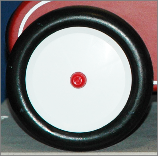
Creating a Shading Network for the Wheels

Refer to Figure 7-47 to observe how the materials are different for the rim and the tire of the wheel. The rim is glossier and has a tighter, sharper specular, whereas the tire has a very diffuse specular and is quite bumpy. You’ll create a Layered shader for the wheels with white feeding into the rim portion and black into the tire portion, instead of assigning to faces like you did earlier with the lamp’s biplane.

Figure 7-47: The tire on the wagon

c07f047.tif

Coloring the Wheel

First you need to determine where the white ends and the black starts on the surface of the wheel mesh.

1. Select the White shader in the Hypershade window. Click the Map icon (c07g003.tif) next to the Color attribute. Right-click the Ramp texture icon, and select Create Texture. The wheel’s color turns to a red, green, blue gradient, but in the wrong direction; you need the gradient to run from the center to the edge and not clockwise across the wheel. In the Ramp texture’s Attribute Editor, set Type to U Ramp, as shown in Figure 7-48.

Figure 7-48: Set the ramp to a U Ramp type.

c07f048.tif

If the ramp doesn’t show up in your view panels, make sure you press 6 to enter Texture Display mode. If the colors and ramp texture still don’t display, make sure Use Default Material isn’t checked in the view panel’s Shading menu.

2. Now the color gradient is running from the center (red) to the outside edge (green) to blue on the reverse side of the wheel. Move the blue ramp’s handle in the ramp’s Attribute Editor until its Selected Position value is about 0.6, as shown in Figure 7-49.

Figure 7-49: Move the blue handle.

c07f049.tif
3. Delete the red handle in the ramp by clicking the checked box on the right of the handle. Change the blue color to black and the green color to white. Set the Interpolation attribute (found above the ramp color) to None so you get clean transitions from white to black, instead of a soft linear gradient where the black slowly grades to white. Name this ramp wheelPositionRamp.
4. The backs of the wheels are solid black. In the wheelPositionRamp, click toward the top of the ramp to create a new color. Set that color to white, and set its position to about 0.920 to place white behind the wheels, keeping the black only where the tire is. See Figure 7-50.

Figure 7-50: Setting the tire location using a ramp

c07f050.tif
Now that you’ve pinpointed where the white rim ends and the black tire begins, you’ll use this ramp as a transparency texture to place the Tire shader on top of the Rim shader in a Layered shader that you’ll create later.
5. You don’t need this Ramp shader on the color of the shader anymore—you did this so you could easily see the ramp color positions in the view panels. In the Hypershade, select the White shader, and click the Input And Output Connections icon (c07g002.tif) to graph the shader, as shown in Figure 7-51.

Figure 7-51: The White shader has the ramp attached as color.

c07f051.tif
6. In the Attribute Editor, RMB+click the Color attribute, and select Break Connection from the context menu to disconnect the ramp from the color. Set the Color back to white. Notice that the link connecting the Ramp texture node to the White shader node disappears in the Hypershade window.
7. Create a Layered shader. MMB+drag the White shader from the Hypershade to the top of the Layered Shader Attributes window, as shown in Figure 7-52. Delete the default Green shader in the Attribute Editor by clicking the checked box below its swatch.

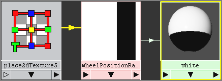
Figure 7-52: Drag the White shader to the Layered shader, and delete the default Green shader from it.

c07f052.tif
8. Create a new Blinn shader, and set its color to black. Name the shader tireShader. Select the Layered shader, and then MMB+drag the new tireShader from the Hypershade to the Layered shader’s Attribute Editor, placing it to the left of the White shader, as shown in Figure 7-53. Name the Layered shader wheelShader.

Figure 7-53: Add the black tireShader.

c07f053.tif
9. Select the wheels, and assign the wheelShader Layered shader to them. The wheels should appear all white. This is where the ramp you created earlier (wheelPositionRamp) comes into play.
10. Select the wheelShader, and click Input And Output Connections to graph the network in the Work Area of the Hypershade window. In the top panel of the Hypershade, click the Texture tab to display the texture nodes in the scene so you can see wheelPositionRamp’s node.
11. In the wheelShader’s Attribute Editor, click the tireShader swatch on the left. MMB+drag the wheelPositionRamp node to the Transparency attribute, as shown in Figure 7-54.

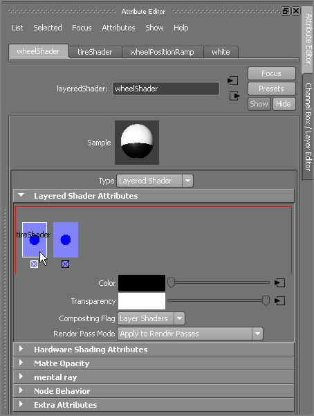
Figure 7-54: Attach the ramp to the Transparency attribute of the tireShader in the wheelShader.

c07f054.tif
12. When you attach the ramp, the wheelShader icon turns white on top and black on the bottom. Render a frame in the persp view panel to make sure the black tires line up properly, as shown in Figure 7-55. The wheel coloring is complete!

Figure 7-55: The tires are done!

c07f055.tif

Hey, Hold on a Minute
Why did you go through a Layered shader with two different shaders (one white and one black) when you could more easily use one shader and assign the same black-to-white ramp to its color? You did this because the white rim and the black tire are different materials, and you need to use two different shaders to properly show that in renders.

Setting the Feel for the Materials and Adding a Bump Map

Because the material look and feel on the real wheels differs quite a bit between the rim and the tire, you’ll further tweak the white rim and the black tire shaders. The rim is a smooth, glossy white, and the tire is a bumpy black with a broad specular. Follow these steps:

1. Let’s set up a good angle of view for your test renders. Position your persp view panel to resemble the view in Figure 7-56. Render a frame.

Figure 7-56: Set your view to this angle, and render a frame.

c07f056.tif
2. Select the White shader, and set Eccentricity to 0.05 and Specular Roll Off to 0.5. Doing so sharpens the specular highlight on the rim.
3. Select the black tireShader, and set Eccentricity to 0.375 and Specular Roll Off to 0.6 to make the highlight more diffuse across the tire. Set Reflectivity to 0.05. Render a frame, and refer to Figure 7-57 to see how the specular highlight is broader and less glossy than in Figure 7-56.

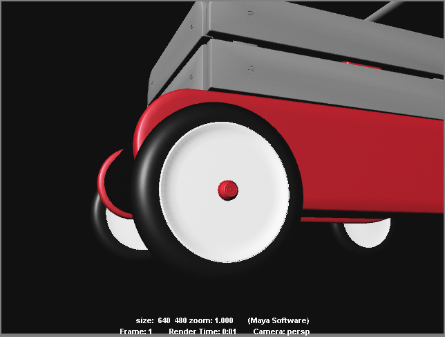
Figure 7-57: Setting specular levels

c07f057.tif
4. Open the Attribute Editor for the tireShader, and click the Map icon (c07g003.tif) next to the Bump Mapping attribute. In the Create Render Node window, click to create a Fractal texture map. Notice that the entire wheelShader icon becomes bumpy. Render a frame, and you’ll see that the entire wheel is bumpy—not just the tire. (See Figure 7-58.) Argh!

Figure 7-58: The whole wheel becomes bumpy!

c07f058.tif
5. You have to use the wheelPositionRamp to prevent the bump from showing on the rim. Select the wheelShader, and click the Input And Output Connections icon (c07g002.tif) in the Hypershade to graph its network (Figure 7-59).

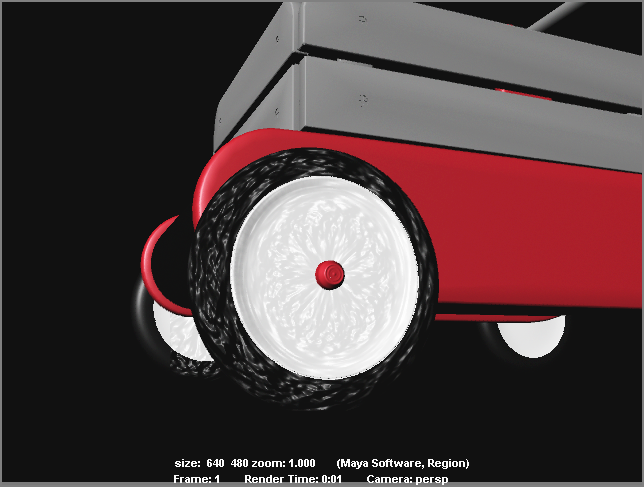
Figure 7-59: Graph the wheelShader network.

c07f059.tif

Notice the single, blue connecting line between the fractal1 node and the bump2d1 node in the Hypershade. This means the alpha channel of the fractal feeds the amount of bump that is rendered on the tireShader. You have to alter the alpha coming out of the fractal node with the positioning ramp to block the rim from having any bump. The white areas of the ramp allow the bump map from the fractal to show on the tire, whereas the black area of the ramp keeps any bump from appearing. Because you already used this ramp to position the Rim shader and the Tire shader on the wheel, it will work perfectly for the bump position as well.

6. You have to use the wheelPositionRamp to prevent the bump from showing on the rim. Select the wheelShader, and click the Input And Output Connections icon (c07g002.tif) in the Hypershade to graph its network (Figure 7-59).
7. Select the fractal to display it in the Attribute Editor, and MMB+drag the wheelPositionRamp in the Hypershade to the Alpha Gain attribute for the fractal, as shown in Figure 7-60.

Figure 7-60: MMB+drag the ramp to the Alpha Gain attribute of the fractal.

c07f060.tif
8. Render a frame, and you see that now the tire has no bump and the rim is bumpy (Figure 7-61).

Figure 7-61: The tire is smooth, and now the rim is bumpy.

c07f061.tif
9. This is easy enough to fix. All you need to do is reverse the ramp and then feed it into the Alpha Gain attribute of the fractal so that the tire is bumpy and the rim is smooth. In the Hypershade, in the Create pane on the left, click the Maya ⇒ Utilities heading, and then click the Reverse icon to create a reverse node in the Hypershade window. See Figure 7-62.

Figure 7-62: Create a reverse node.

c07f062.tif
10. In the Hypershade, MMB+drag the wheelPositionRamp node onto the Reverse node, and select Input from the context menu when you release the mouse button. This connects the output of the ramp into the reverse node, which will then reverse the effect of the ramp on the fractal when you connect it in the next step.
11. MMB+drag the reverse node on top of the fractal1 node, and select Other from the context menu. This opens the Connection Editor, which you first saw in Chapter 3. On the left the reverse1 node is loaded, and on the right is the fractal1 node. In the left pane, click the plus sign next to the Output attribute, and select outputX. In the right pane, select the alphaGain attribute, as shown in Figure 7-63.

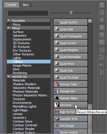
Figure 7-63: Connecting the reverse node to the fractal node

c07f063.tif
12. Open the Render Settings window by choosing Window ⇒ Rendering Editors ⇒ Render Settings. Click the Maya Software tab, and set Quality to Production Quality in the pull-down menu. (See Figure 7-64.) Render a frame: you finally have a bump on the tire and a smooth rim. See Figure 7-65.

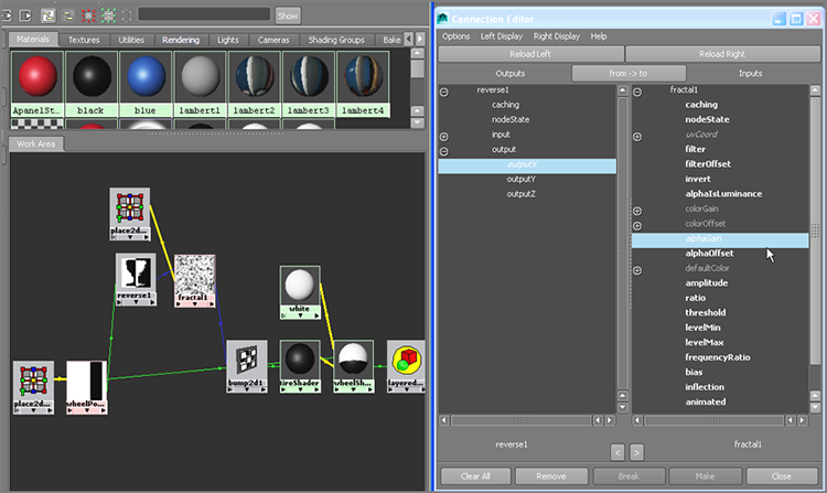
Figure 7-64: Set Quality to Production Quality.

c07f064.tif

Figure 7-65: Now you have the bump where you need it.

c07f065.tif
13. It’s not a very convincing bump yet, so select the fractal node, and set Ratio to 0.85. Click the Placement tab for the fractal (it should be called something like place2dTexture6), and set the Repeat UV values to 18 and 48, as shown in Figure 7-66. Doing so makes the fractal pattern finely speckled on the tire.

Figure 7-66: Set the Repeat UV values for the fractal map.

c07f066.tif
14. Render a frame; the fractal’s scale on the bumpy tire looks too strong. Double-click the bump2d node in the Hypershade, and in the Attribute Editor, set Bump Depth to 0.04. Render, and check your frame against Figure 7-67. The bump looks much better, if not a little strong from this angle; you can finesse it to taste from here.

Figure 7-67: The wheel looks pretty good.

c07f067.tif

Tire Summary

Congratulations! You’ve made your first somewhat complex shading network, as shown in Figure 7-68. By now, you should have a pretty good idea of how to get around the Hypershade and create shading networks. To recap, you’re using a ramp to place the two Tire and Rim shaders on the wheel, as well as using it to place the bump map on just the tire by using a reverse node. The more you make these shading networks, the easier they will become to create.

Figure 7-68: Your first complex shading network

c07f068.tif

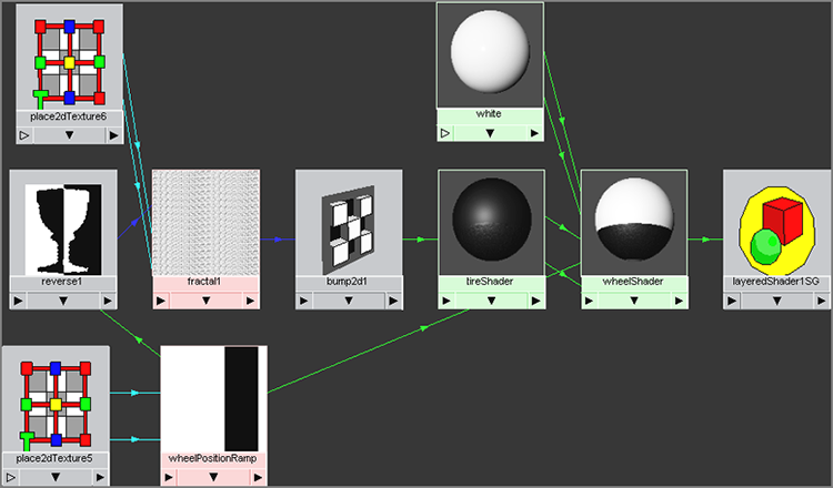
This type of shading is called procedural shading, because you used nothing but stock Maya texture nodes to accomplish what you needed for the wheels. In the following sections, you’ll make good use of image mapping to create the decals for the wagon body as well as the wood for the railings.

You can load the file RedWagonTexture_v01.ma from the Scenes folder of the RedWagon project to check your work or skip to this point.

Putting Decals on the Body

Figure 7-69 shows you the decals that need to go onto the body of the wagon. They include the wagon’s logo, which you’ll replace with your own graphic design, and the white stripe that lines the side panels.

Figure 7-69: You need to add the body decals.

c07f069.tif

Instead of trying to make a procedural texture as you did with the wheel, you’ll create an image map that will texture the side panels’ white stripe. The stripe is far too difficult to create otherwise. You’ll create an image file using Photoshop (or another image editor) to make sure the white stripe (and later the red wagon logo) lines up correctly.

Working with UVs

Mapping polygons can involve the task of defining UV coordinates for them so that you can more easily paint an image map for the mesh. When you create a NURBS surface, UV coordinates are inherent to the surface. At the origin (or the beginning) of the surface, the UVcoordinate is (0,0). When the surface extends all the way to the left and all the way up, the UV coordinate is (1,1). When you paint an 800×600–pixel image in Photoshop, for example, it’s safe to assume that the first pixel of the image (at X = 0 and Y = 0 in Photoshop) will map directly to the UV coordinate (0,0) on the NURBS surface, whereas the top-right pixel in the image will map to the UV (1,1) of the surface. Toward that end, mapping an image to a NURBS surface is fairly straightforward. The bottom of the image will map to the bottom of the surface, the top to the top, and so on. Figure 7-70 shows how an image is mapped onto a NURBS plane and a NURBS sphere.

Figure 7-70: An image file is mapped to a NURBS plane and a NURBS sphere. Notice the locations marked in the image and how they map to the locations on the surface, with the pixel coordinates directly corresponding to the surface’s UV coordinates.

c07f070.tif

The locations in the image, marked by text, correspond to the positions on the NURBS plane. The sphere, because it’s a surface bent around spherically, shows that the origin of the UV coordinates is at the sphere’s pole on the left and that the image wraps itself around it (bowing out in the middle) to meet at the seam along the front edge as shown.

When you’re creating polygons, however, this isn’t always the case. You must sometimes create your own UV coordinates on a polygonal surface to get a clean layout on which to paint in Photoshop. Although poly UV mapping becomes fairly involved and complicated, it’s a concept that is important to grasp early. When poly models are created, they have UV coordinates; however, these coordinates may not be laid out in the best way for texture-image manipulation.

Working with the A Panels

Let’s look at how the UVs are laid out for the A panel of the wagon model. Use Figure 7-42 earlier in the chapter to remind yourself where the A panel is.

1. Using the scene file RedWagonTexture_v01.ma from the Scenes folder of the RedWagon project, select the A panel on one side of the wagon, and choose Window ⇒ UV Texture Editor, as shown in Figure 7-71.

Figure 7-71: The A panel in the UV Texture Editor

c07f071.tif

This section assumes you have some working knowledge of Adobe Photoshop. You can skip the creation of the maps and use the maps already on the companion web page, which are called out in the text later in the exercise.

The UV Texture window works almost like any other view panel. You may navigate the window and zoom in and out using the familiar Alt+mouse button combinations.
2. RMB+click any part of the wireframe layout in the UV Texture Editor window, and select UV to enter the UV selection. Select the entire wireframe mesh at the lower right, as shown in Figure 7-72. Notice that green points are selected—almost as if they were vertices. These are UV points, and they’re what define the UV coordinates on that part of the mesh. Look in the perspective view panel; the entire front face of the A panel is selected as well as the green UV points (also in Figure 7-72).

Figure 7-72: Select the UVs on this part of the A panel mesh.

c07f072.tif
Feel free to select parts of the UV layout in the UV Texture Editor to see what corresponding points appear on the mesh in the persp view panel. This will help orient you as to how the UV layout works on this mesh.
3. You need to again lay out just this area of the mesh’s UVs. Because you already have the entire front side of the panel selected in UVs, let’s convert that selection to poly faces on the model. In the Polygons menu set and in the Maya Main Menu bar, choose Select ⇒ Convert Selection ⇒ To Faces. The front faces of the A panel mesh are selected, as shown in Figure 7-73. You can always manually select just the front faces of the mesh, but this conversion method is much faster. The UV Texture Editor shows just those faces now.

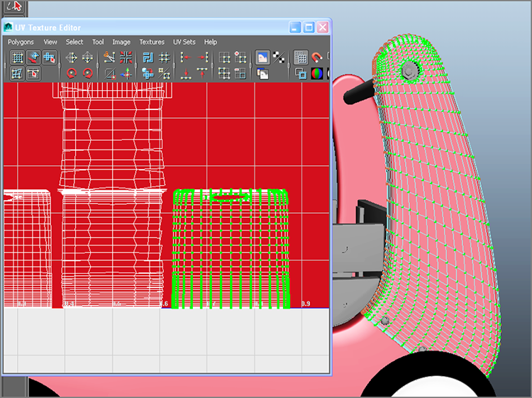
Figure 7-73: Convert the UVs you just selected to a face selection. This method easily isolates the front faces of the A panel for you to lay out their UVs again.

c07f073.tif
4. With those faces selected, make sure you’re in the Polygons menu set. Choose Create UVs ⇒ Planar Mapping optionbox.png from the Main Menu bar. In the option box, set the Project From option to X Axis, check the Keep Image Width/Height Ratio option, and then click Project. (See Figure 7-74.) The UV Texture Editor shows the front A panel face.

Figure 7-74: Create a planar projection for the UV layout.

c07f074.tif
5. Now the front face has a much simpler UV layout from which to paint. However, it’s centered in the UV Texture Editor and will overlap the other UVs of the same mesh. You should move and size it to fit into its original corner, more or less, to make sure no UVs double up on each other. In the UV Texture Editor, right-click the wireframe, and select UV to enter UV selection. Select all the UVs on those faces; all the UVs for the A panel mesh appear in the UV Texture Editor, and you can see the overlap. See Figure 7-75.

Figure 7-75: The UVs for the A panel, with the front side’s UVs still selected

c07f075.tif
6. Press W for the Move tool, and move the selected UVs to the side of the UV Texture Editor. Press R for the Scale tool, and scale them down a bit to fit into the corner, as shown in Figure 7-76.

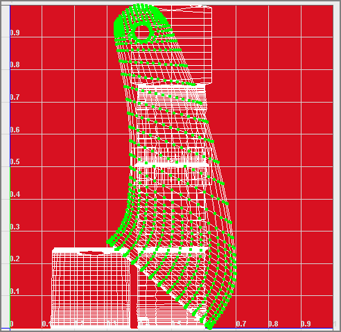
Figure 7-76: Position these UVs to make sure they don’t overlap the rest of the A panel mesh’s UVs.

c07f076.tif
7. Earlier in the chapter, you saw how to write out a PSD file with a UV snapshot as one of its layers. You’ll use a similar technique to paint the decal for the panel. Click an empty area of the UV Texture Editor to deselect everything. Then, in Object Selection mode (press F8 if you need to exit Component Selection), select the A panel mesh in the persp view panel.
8. In the UV Texture Editor window, select Polygons ⇒ UV Snapshot to open the option box. Set both Size X and Size Y to 1024. Change the image format to TIFF, click the Browse button at the top next to the File Name field, and navigate to the RedWagon project’s Sourceimages folder on your hard drive. Name the file ApanelUV.tif, and click Save. Leave UV Range set to Normal (0 to 1), and click OK. See Figure 7-77.

Figure 7-77: Settings for the UV snapshot

c07f077.tif

Working in Photoshop

Next, you’ll go into Photoshop to paint your map according to the UV layout you just output.

1. In your OS file browser, navigate to the RedWagon project’s Sourceimages folder, and open the file ApanelUV.tif in Photoshop. Figure 7-78 shows the layout of the UVs that you’ll use to create the white stripe for the front of the A panel.

Figure 7-78: Using a UV snapshot makes working with the UV layout for the A panel easy.

c07f078.tif
2. In Photoshop, create a new layer on top of the background layer that is the UV layout (white on black, as shown). Using the Bucket tool, fill that new layer with the same red you used on the shader in your scene. To do so, click the foreground color swatch in Photoshop, and set H to 355, S to 91 percent, and B to 65 percent, as shown in Figure 7-79. Click OK.

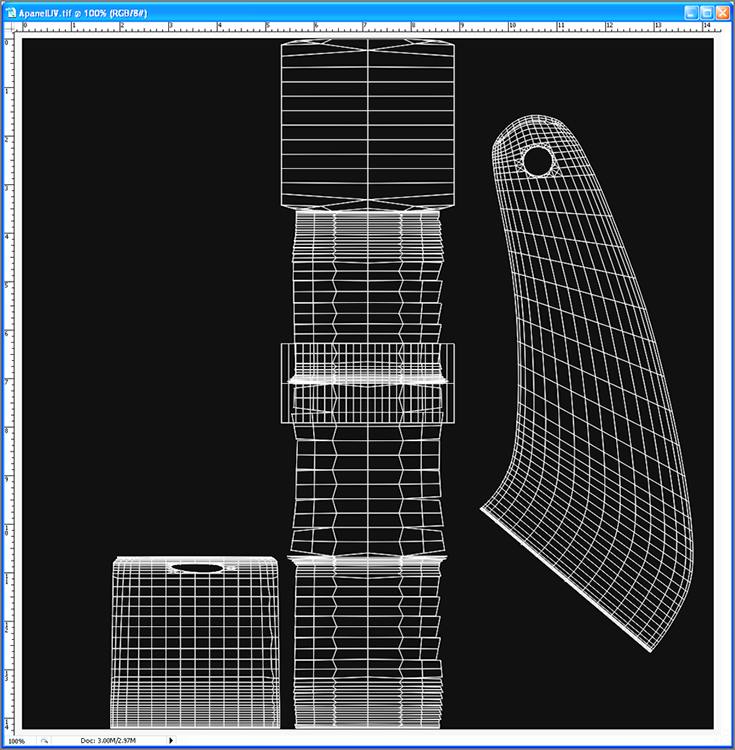
Figure 7-79: In Photoshop’s Color Picker, create the same red you used for the wagon.

c07f079.tif
3. Using the Bucket tool, click to fill the entire image with the red you just created. The trouble is that now you can’t see the UV layout. Set the Opacity value of the red layer in Photoshop to 50 percent, as shown in Figure 7-80.

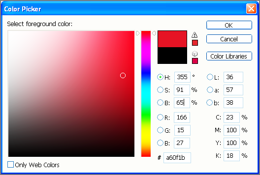
Figure 7-80: Set the opacity for the red layer in Photoshop so you can see the UV layout on the layer below.

c07f080.tif
4. Set Photoshop’s foreground color to white. Using the Line and Brush tools set to a width of about 6 pixels, draw a stripe following the UV layout lines, as shown in Figure 7-81. Doing so places that white stripe along the A panel’s outer edge, because the UV lines you’re following correspond to that area of the mesh. The rest will be left red.

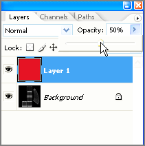
Figure 7-81: Follow the UV lines to draw the white stripe.

c07f081.tif
5. You may have drawn directly on the red layer in Photoshop or created a new layer for the stripe. In either case, set the Opacity value of the red layer back to 100 percent so you can no longer see the UV layout. Your image file should look like the one in Figure 7-82. Save the image as ApanelStripe.tif in the Sourceimages folder of your RedWagon project. You may keep the layers in the TIFF file, or you may choose to flatten the image or merge the layers. It may be best to keep the stripe and red on separate layers so that you can go back into Photoshop and edit the stripe as needed.

Figure 7-82: The striped image file

c07f082.tif

Creating and Assigning the Shader

Now, let’s create the shader and get it assigned to the geometry.

1. In Maya, open the Hypershade, and select the Red shader. Duplicate it by choosing Edit ⇒ Duplicate ⇒ Shading Network in the Hypershade window, as shown in Figure 7-83.

Figure 7-83: Duplicate the original Red shader.

c07f083.tif
2. Name the new shader (called red1) ApanelStripe. Open the Attribute Editor, click the Map icon (c07g003.tif) next to Color, and choose File. In the Attribute Editor, click the Folder icon next to the Image Name field. Navigate to your Sourceimages folder, and select ApanelStripe.tif, as shown in Figure 7-84.

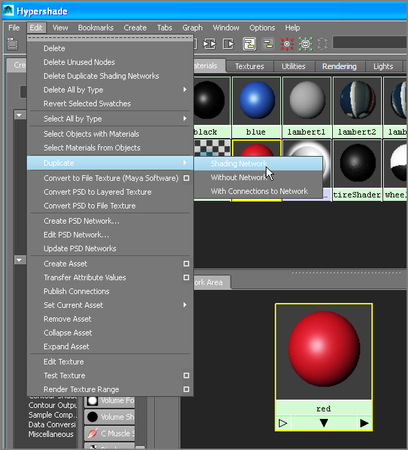
Figure 7-84: Select the ApanelStrip.tif file.

c07f084.tif
3. In the Hypershade, you may see that the Shader icon has turned somewhat transparent. Maya is automatically mapping the Transparency attribute of the shader as well as the color. Double-click the shader to open its Attribute Editor, RMB+click Transparency, and select Break Connection from the context window. Doing so sets the shader to the same red you used earlier, but now it gives you a stripe along the side A panel.
4. Assign the ApanelStripe shader to the A panel mesh, and press 6 for Texture Display mode in the persp view panel. See Figure 7-85. The stripe lines up well.

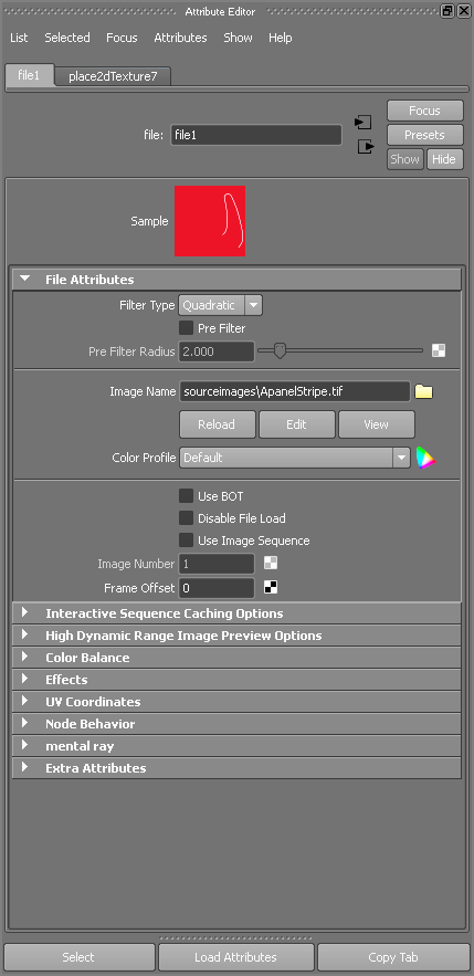
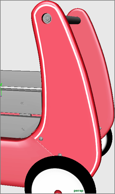
Figure 7-85: The stripe

c07f085.tif

You may skip the image creation using Photoshop and use the ApanelStripe.tif image file found in the Sourceimages folder of the RedWagon project on the companion web page instead.

Copying UVs

You need to put the stripe on the other side’s A panel. Select the other A panel, and assign the ApanelStripe shader to it. You’ll notice that no stripe appears. (See Figure 7-86.) This is because the UV layout for this A panel hasn’t been set up yet. Don’t worry; you don’t have to redo everything you did for the first A panel. You can essentially copy the UVs from the first A panel mesh to this one.

Figure 7-86: Assign the ApanelStripe shader to the other side’s A panel.

c07f086.tif
1. Select the first A panel (with the stripe) and the second panel (without the stripe). In the Polygons menu set, choose Mesh ⇒ Transfer Attributes optionbox.png. In the option box, set Sample Space to Local, as shown in Figure 7-87, and click Transfer.

Figure 7-87: The Transfer Attributes settings

c07f087.tif
2. The stripe appears on the inside of the back A panel, not on the outside as you need. Select that A panel, and choose Modify ⇒ Center Pivot.
3. In the Channel Box, enter a value of –1.0 for Scale X. The stripe flips to the correct side, as shown in Figure 7-88.

Figure 7-88: The stripe is on the correct side now.

c07f088.tif
4. With that A panel still selected, choose Modify ⇒ Freeze Transformations.

You can load the file RedWagonTexture_v02.ma from the Scenes folder of the RedWagon project to check your work or skip to this point.


The file texture you’ll use for the panels was painted in Photoshop to place the stripes and logo properly on the wagon using their UV layouts. Study the image file, and see how it fits on the mesh of the wagon. Try adjusting the image file with your own artwork to see how your image map affects the placement on the mesh.

Working with the B Panels

With the A panels done, you’ll move on to the B panels (Figure 7-42 earlier in the chapter), using much the same methodology you did with the A panels. To begin, follow these steps:

1. Select one of the B panels, shown in Figure 7-89, and open the UV Texture Editor window.

Figure 7-89: Starting on the B panels

c07f089.tif
2. As you did with the front face of the A panel, select the UVs on the lower-right side of the layout in the UV Texture Editor, as shown in Figure 7-90, to isolate the front face of the B panel.

Figure 7-90: Select the front face UVs for the B panel.

c07f090.tif
3. Choose Select ⇒ Convert Selection ⇒ To Faces. You’ve isolated the front face of the B panel.
4. Choose Create UVs ⇒ Planar Mapping optionbox.png. In the option box, set the Project From option to X Axis, and make sure the Keep Image Width/Height Ratio option is checked, just as before. Your B panel shows up nicely laid out in the UV Texture Editor. See Figure 7-91.

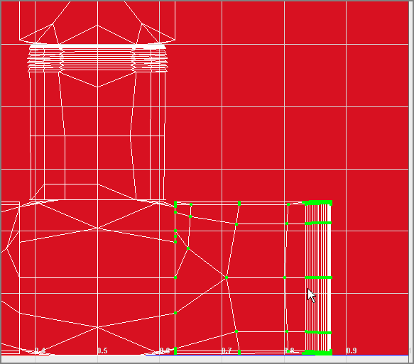
Figure 7-91: The planar projection creates a nice UV layout for the front faces of the B panel.

c07f091.tif
5. Convert the selection to UVs, and use Move (W), Scale (R), and Rotate (E) to position the UV layout for that front face, as shown in Figure 7-92.

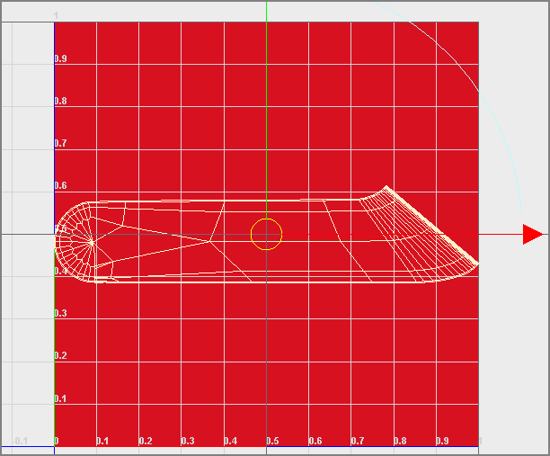
Figure 7-92: Put the front face UVs on the side.

c07f092.tif
6. Press F8, and select the B panel mesh. In the UV Texture Editor, save a UV snapshot called BpanelUV.tif to theSourceimages folder of the RedWagon project.
7. Open the BpanelUV.tif image in Photoshop, and follow the same steps as you did for the A panel to lay down a red layer and paint a stripe along the layout, as shown in Figure 7-93. It’s best to save the stripe on its own layer in Photoshop, because you’ll probably need to edit and reposition the stripe to make sure it lines up with the A panel stripe after you assign the shader.

Figure 7-93: Create the B panel’s stripe in Photoshop using the UV snapshot.

c07f093.tif
8. Create your own logo to place in the middle of panel B, and place it in the Photoshop image file, as shown in Figure 7-94. Save the image file as BpanelStripe.tif into the Sourceimages folder.

Figure 7-94: Create the logo in Photoshop.

c07f094.tif
9. Duplicate another Red shader, and, as you did previously, assign the BpanelStripe.tif as its color map. If necessary, disconnect the transparency from the shader as you did with the A panel’s shader. Name the shader BpanelStripe.
10. Assign the BpanelStripe shader to the B panel, as shown in Figure 7-95.

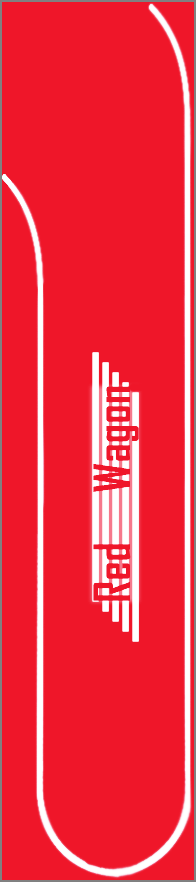
Figure 7-95: The B panel has its decals.

c07f095.tif

You can skip the image creation in Photoshop and use the BpanelStripe.tif image file found in the Sourceimages folder of the RedWagon project on the companion web page.

Creating the Other B Panel Texture

Finally, you need to create the shader for the other side’s B panel. Assign the BpanelStripe shader to the other B panel. Nothing happens, because the UVs for the second B panel aren’t set up yet.

However, because there is a logo with text, setting up its UVs won’t be as simple as copying the UVs from the first B panel and then mirroring the mesh, as you did with the A panel with a Scale X value of –1.0. Doing so will make the logo and text read backward. First you’ll copy and flip the UVs to the other B panel.

1. Select the first B panel with the correct texture, and then select the other side’s B panel and choose Mesh ⇒ Transfer Attributes optionbox.png. Make sure Sample Space is still set to Local, and set Flip UVs to U. Click Transfer to copy the UVs, flipping them over, as you can see in Figure 7-96.

Figure 7-96: Copying and flipping the UVs to the other B panel

c07f096.tif
2. You have to go back to Photoshop and create a second BpanelStripe.tif image file with a mirrored logo. In Photoshop, create a marquee around the logo, and mirror or flip the canvas horizontally. See Figure 7-97.

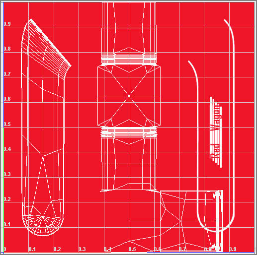
Figure 7-97: Flip the original image horizontally to fit the new UV layout of the second B panel.

c07f097.tif
3. Select the logo portion of the image and flip that vertically, as shown in Figure 7-98. Save the image as BpanelStripe_2.tif.

Figure 7-98: Flip the logo vertically, and save the image as its own file.

c07f098.tif
4. Duplicate the BpanelStripe shader in the Hypershade by selecting the shader and choosing Edit ⇒ Duplicate ⇒ Shading Network. The copy is called BpanelStripe1.
5. Select the newly copied BpanelStripe1 shader, and graph its input and output connections (c07g002.tif) in the Hypershade. Select its file node, and open the Attribute Editor. Click the Folder icon to select a new image file, and then select the BpanelStripe_2.tif you just created in the Sourceimages folder. See Figure 7-99.

Figure 7-99: Assign the new image file to the new BpanelStripe1 shader.

c07f099.tif
6. The stripe and logo display on the wrong side of the B panel. Select the mesh, and center its pivot.
7. Set the Scale X attribute for the B panel to –1.0 to mirror it. The stripe and logo decals now show up on the correct side of the panel. Select the mesh and freeze its transforms. Figure 7-100 shows the wagon so far.

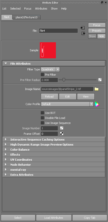
Figure 7-100: The wagon has decals on both sides.

c07f100.tif

Texturing the Floor

Right now, the floor of the wagon is red, like the rest of its body. However, the real wagon has a blue floor, not red. If you select the mesh for the wagon’s floor (named wagonFloor) and assign the Blue shader you created, the whole body of the wagon turns blue, and that isn’t what you want. You need only the inside and bottom of the floor to be blue, not the front and back sides of the wagon’s body.

You’ll make a face assignment instead of dealing with UVs and image files. RMB+click the wagon floor mesh, and select Face from the marking menu. Select the two faces for the floor, as shown in Figure 7-101.

Figure 7-101: Select the floor faces.

c07f101.tif

With the faces selected, assign the Blue shader from the Hypershade window, and you’re finished! You have a blue floor. All that remains now are the screws, bolts, handle, and wood railings.

You can load the file RedWagonTexture_v03.ma from the Scenes folder of the RedWagon project to check your work or skip to this point.

Shading the Wood Railings

You’ll use procedural shading to use the Wood texture available in Maya to create the wood railings. Begin here:

1. In the Hypershade, create a new Phong material.
2. Click the Color Map icon (c07g003.tif), and choose the Wood texture from the 3D Textures heading in the Create pane in the Hypershade.
3. In the Attribute Editor for the Wood texture, set the Filler Color and Vein Color attributes according to Table 7-3.

Table 7-3: Filler Color and Vein Color attributes

Table 07-03
4. Set Vein Spread to 0.5, Layer Size to 0.5, Randomness to 1.0, Age to 10.0, and Grain Contrast to 0.33. In the Noise Attributes heading, set Amplitude X to 0.2 and Amplitude Y to 0.1, as shown in Figure 7-102. Name the shader Wood.

Figure 7-102: Setting the Wood texture

c07f102.tif
5. Select all the wood railings and posts, and assign the Wood shader to them. Render a frame, and compare it to Figure 7-103. Notice the green cube place3dTexture node that is now in your scene. See Figure 7-104.

Figure 7-103: Assign the Wood shader.

c07f103.tif

Figure 7-104: The place3dTexture node for the wood texture

c07f104.tif
6. The side wood railings look fine; however, the wavy pattern on the front and back wood railings looks a bit odd. In the Hypershade, duplicate the shading network for the Wood shader, and call the new shader woodFront.
7. Assign that shader to the front and back railings and posts. Graph the network on the woodFront shader in the Hypershade window.
8. In the Hypershade, select the place3dTexture2 node (Figure 7-105) and the green cube in the view panels.

Figure 7-105: Select the placement node for the second Wood texture.

c07f105.tif
9. Rotate that placement node in the persp view panel 90 degrees to the right or left. Render a frame, and compare it to Figure 7-106. The wood should no longer have that awkward wavy pattern.

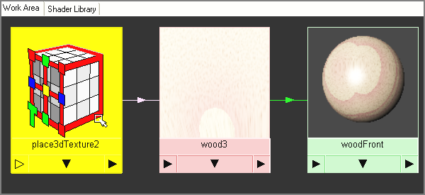
Figure 7-106: The wood on the front and back railings looks better.

c07f106.tif

The wood railings are finished. Now, for some extra challenge, you can use pictures of real wood to map onto the railings for a more detailed look. The procedural Wood texture can give you only so much realism. If you create your own wood maps, use your experience with the side panels to create UV layouts for the railings so you can paint realistic wood textures using Photoshop. You’ll use custom photos and texture image maps next to simulate the rich wood in the decorative box later in the chapter.

Finishing the Wagon

Now that the railings are done and you have test renders, there are only two parts left to texture: the bullnose front of the wagon, and the metal handle and screws. From here, take your time and create a bump map based on a fractal, as you did for the tires, and apply it to the bullnose’s black shader. Figure 7-107 shows a nice subtle bump map on the bullnose.

Figure 7-107: A nice bump for the bullnose

c07f107.tif

And last, you’ll need a metal shader for the screws, bolts, and handlebar for the wagon. Use a Phong shader with a blue-gray color and a low diffuse value, and assign it to all the metal parts of the wagon, as shown in Figure 7-108. You can then add an environment map to the reflection color like you did for the table lamp stem earlier in this chapter to give the metal a reflective look.

Figure 7-108: Select all the metal screws, the bolts, and the handlebar, and assign the Metal shader to them.

c07f108.tif

Because metal is a tricky material to render and a lot of a metal’s look is derived from reflections, you’ll finish setting the Metal shader’s attributes in Chapter 11, when you render the wagon as well as the table lamp. You’ll enable raytracing to get realistic reflections and gauge how to best set up the Metal shader for a great look.

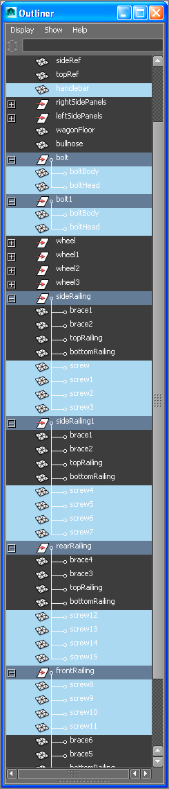
Figure 7-109 shows the wagon with all its parts assigned to shaders. Figure 7-110 shows a quick render of the wagon as it is now.

Figure 7-109: The wagon in the Perspective panel

c07f109.tif

Figure 7-110: A current render of the wagon

c07f110.tif

You can load the file RedWagonTexture_v04.ma from the Scenes folder of the RedWagon project to check your work or skip to this point.

Photo-Real Mapping: The Decorative Box

With all the references you can find to any given object on the Internet, why not use real photos to create the textures for a model? That’s exactly what you’ll do here, with the decorative box you modeled in Chapter 3, using pictures of the real box.

You’ll take this texturing exercise one important step further in Chapter 11 and experience how you can add detail to an object through displacement mapping, after you assign the colors in this chapter. This will allow you to add finer detail to a model without modeling those details.

Setting Up UVs (Blech!)

The UVs on the decorative box aren’t too badly laid out by default, as you can see in Figure 7-111. The only parts of the box that are missing in the UV layout are the feet. That is a common issue when extruding polygons: their UVs are rarely laid out automatically as you extrude them. Frequently, they’re bunched up together in a flat layout that is difficult, if not impossible, to see in the UV Texture Editor.

Figure 7-111: The feet UVs are missing from the box model.

c07f111.eps

Open the file boxModel_v07.mb in the Scenes folder of the Decorative_Box project on the companion web page, or continue with your own model.

First you have to make room for the feet UVs.

1. Select all the UVs for the entire box in the UV Texture Editor. Press R for the Scale tool, and scale everything down uniformly to gain some space in the normalized UV space, shown in Figure 7-112.

Figure 7-112: Scale all the UVs down a bit.

c07f112.tif
2. Now for the tedious part. You have to create new UVs for the four feet and then move them to where they should be in the full box’s UV layout. Go into Component mode, and select the poly faces for the four feet, as shown in Figure 7-113.

Figure 7-113: Select the faces for the feet.

c07f113.tif
3. With the faces selected, go to the main Maya window. In the Polygons menu set, select Create UVs ⇒ Automatic Mapping. The feet now have UVs that you can see in Figure 7-114. However, they’re all over the place. You have to individually select and move each face of each foot to its appropriate place on the box’s overall UV layout.

Figure 7-114: The automatic UV creation puts the UVs everywhere.

c07f114.tif
4. Select all the feet UVs in the UV Texture Editor, scale them all down uniformly together. You want to scale them all so that one of the squares fits into the corner of the top shape, as shown in Figure 7-115 (left). Then move them all together off to the side, as shown in Figure 7-115 (right). You’ll position and scale them to fit properly soon.

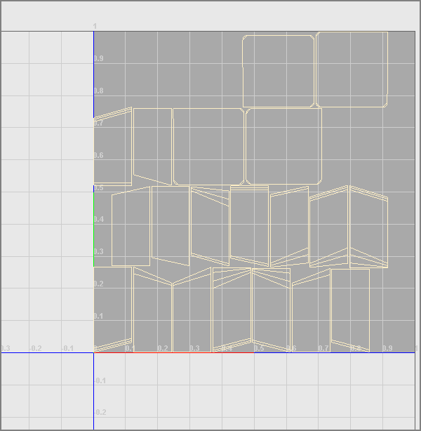
Figure 7-115: Scale the feet UVs to fit the size of the rest of the box’s UVs (left).Then move the feet UVs to the side of the UV editor (right).

c07f115.tif

Laying out UVs can be a time-consuming affair, as you’ve seen with the wagon. Although it’s recommended that you follow along with this exercise to lay out UVs for the box (because doing so will give you more practice and experience with UVs), you can skip straight to color-mapping the box in the next section by downloading the file boxTexture01.mb in the Scenes folder of the Decorative_Box project on the companion web page.

5. Now comes the task of figuring out which UV fits where. In the UV Texture Editor window, select the edges shown in Figure 7-116 by Shift+single-clicking them. Do not use a marquee selection to make sure you select only the single edges you need. Notice that as you select each edge, they become selected in the model as well as the feet UVs off on the side of the UV Texture Editor window. These are the edges where the outside sides of the feet meet the box. If you find it easier, you can select those edges from the model itself instead of the UV Texture Editor.

Figure 7-116: Select these individual edges either in the model view or in the UV Texture Editor.

c07f116.eps
6. With those edges selected, in the UV Texture Editor choose the Move And Sew The Selected Edges icon (Figure 7-117). This will snap the UVs for the outside sides of the feet to their respective sides on the box. If you did not scale the feet UVs in step 4 well enough, you will notice that the feet will stick out from the sides of the box’s UVs, as shown in Figure 7-118 (left). If that is the case, it’s easier to return to step 4 (press Z for undo until you reach step 4 again) and scale those feet UVs more accurately. This can have a little bit of a back and forth. As long as you are within reasonable size, you will be fine. Figure 7-118 (right) shows a better matching scale of the feet after the UVs are sewn together.

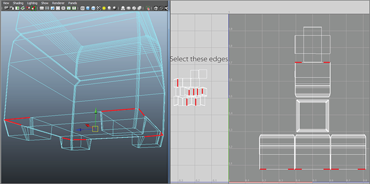
Figure 7-117: The Move And Sew The Selected Edges icon in the UV Texture Editor

c07f117.tif

Figure 7-118: Sew the feet edges to the box. On the left, the feet UVs are scaled too big in step 4. On the right, the feet UVs are scaled properly.

c07f118.tif
7. Right-click in the UV Texture Editor, and select UV from the marking menu. Next, select just one corner UV from the bottom shape of the box, as shown in Figure 7-119 (left). In the UV Texture Editor, choose Select ⇒ Select Shell to select the entire bottom UV shape, and then press W to move the bottom UVs up in the UV Texture Editor a little bit, as shown in Figure 7-119 (right).

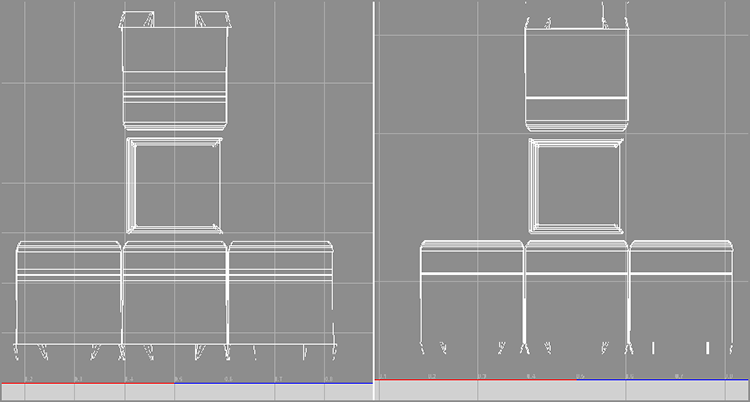
Figure 7-119: Select one UV (left); then select the shell and move the bottom UVs up in the UV Texture Editor (right).

c07f119.tif
8. Figure 7-119 (right) also shows the remaining feet UVs off on the left side of the UV Texture Editor window. The four square shapes are the bottoms of the feet. Select just one corner UVs of the square shown in Figure 7-120 (left); then select the entire shell (Select ⇒ Select Shell) and move it to fit to the bottom UVs of the box as shown in Figure 7-120 (right).

Figure 7-120: Select one UV in the corner (left); then select the shell and move it to fit the box bottom UV shape.

c07f120.tif
9. Repeat step 8 to place all the feet bottom shapes around the UVs of the bottom of the box, as shown in Figure 7-121.

Figure 7-121: Place the feet bottoms to the box bottom and then line up the remaining feet UVs to the side.

c07f121.tif
10. Individually select the shells of the remaining feet UVs on the side of the UV Texture Editor, and line them up to the side of the box bottom as shown in Figure 7-121. Those remaining feet UVs are the inside faces of the feet and share the same generic wood texture as the bottom of the box, so aligning and sewing them together like you did for the outside faces of the feet in steps 5 and 6 is not necessary (Figure 7-122).

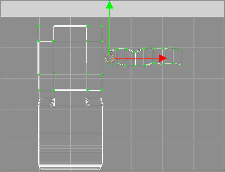
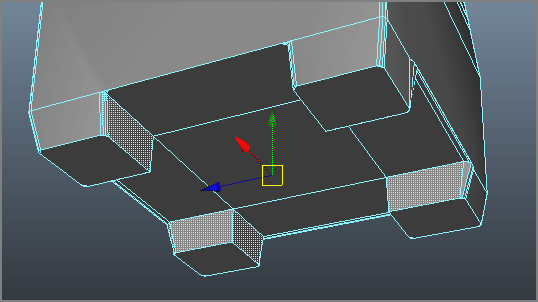
Figure 7-122: These faces will have a generic wood texture like the bottom of the box and do not need to be carefully lined up.

c07f122.tif

When you’ve finished, your UV Texture Editor should resemble the one shown in Figure 7-123. Because the box’s decorations are seamless from the top of the box down to the four sides, let’s lay out the UVs to make painting and editing in Photoshop easier.

Figure 7-123: Finally, you’re finished with the feet UVs.

c07f123.eps

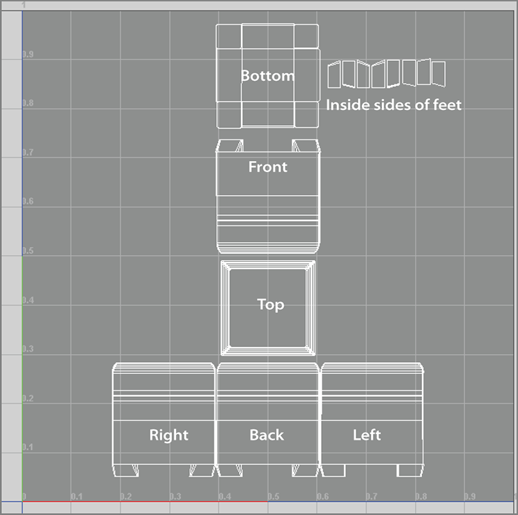
In the UV Texture Editor, select the box top’s edges, as shown in Figure 7-124 (left). Then click the Move And Sew The Selected Edges icon (shown earlier in Figure 7-117) in the UV Texture Editor, and your UV layout should match Figure 7-124 (right). The top and sides of the box are all one UV shell now.

Figure 7-124: Select the box top edges (left), and sew them together (right).

c07f124.eps

UV layout can be an exacting chore, but when it’s completed, you’re free to lay out your textures. You can check your work against the file boxTexture01.mb in the Scenes folder of the Decorative_Box project on the companion web page. You can also take a much needed breather. I sure hope you’ve been saving your work!

Color Mapping the Box

Now that you have a good UV layout, you can output a UV snapshot and get to work editing your photos of the box to make the color maps. Start with the following steps:

1. Select the box, and open the UV Texture Editor window. From the UV Texture Editor menu, select Polygons ⇒ UV Snapshot. In the UV Snapshot window, set Size X and Y to 2048. Change Image Format to TIFF.
Click the Browse button, and select a location for your UV snapshot image. Generally, the project’s Sourceimages folder is the best place for it. Make sure you don’t write over the UV snapshot already created for you. Type in a name for your UV snapshot, and click OK to create the image. Figure 7-125 shows the option box, and Figure 7-126 shows the UV snapshot image.

Figure 7-125: Setting the UV Snapshot options

c07f125.tif

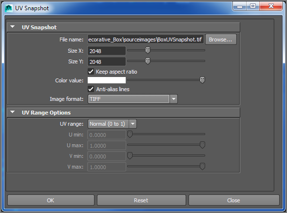
Figure 7-126: The UV snapshot for the decorative box, shown as black lines on white. You may see white lines on black in Photoshop.

c07f126.tif
2. Open the UV snapshot image in Photoshop or your favorite image editor, and set it as its own layer. Rename the layer to UV Snapshot. I’ve done the heavy lifting for you and have prepared five photos of the decorative box that you can use to map the model. Figure 7-127 shows the photos of the box. This image file is included as lineup.jpg in the Sourceimages folder in the Decorative_Box project on the companion web page.

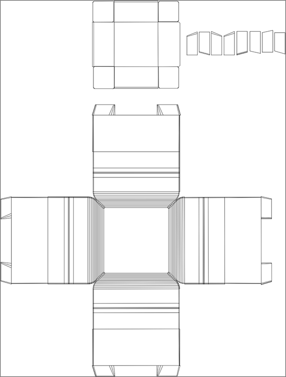
Figure 7-127: Photos of the box

c07f127.eps
3. As you’ve probably guessed, you need to copy and paste the photos to their respective views over the UV Snapshot layer. Open the lineup.jpg file in Photoshop alongside the UV snapshot. Marquee+select a box around the top image (the one at the left in Figure 7-127), and copy it (Ctrl+C or Edit ⇒ Copy in Photoshop).
4. Go to the UV snapshot image in Photoshop, and paste the image on top. Rename the new layer to Box Top, and set the layer’s Opacity to 50% so you can still see the UV layout, as shown in Figure 7-128.

Figure 7-128: Paste the top image onto the UV snapshot image.

c07f128.tif
5. Use the Scale function in Photoshop (Edit ⇒ Transform ⇒ Scale) to move and scale the top image to fit over the top of the UV layout, as shown in Figure 7-129. Make sure you scale the box-top image uniformly to keep it from distorting. You can do this by holding the Shift key as you scale the image up or down.

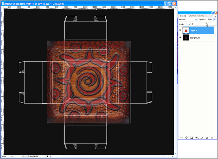
Figure 7-129: Position and scale the top image in Photoshop to line up with the UVs of the top of the model. Notice the overlap of the sides and the top.

c07f129.eps
These photo images of the box have been retouched and painted to create an overlap. This means that parts of the sides of the box show in the top image. As you can see in Figure 7-129, the top image extends slightly all around the four sides. This allows the different parts of the texture map (top and four sides) to overlap and blend with each other better when put on the model.
Save your work as boxColorMap01.psd in the project’s Sourceimages folder. Saving as a Photoshop file will preserve the layers for easier editing.
6. Marquee+select the right-side image of the box (immediately to the right of the top image in lineup.jpg), and copy it. Paste it into boxColorMap01.psd in Photoshop. Do your best to align the right-side image with the top image, using the features of the box to line them up, as you can see in Figure 7-130. You can fix this later by adjusting both the map and the UVs on the box for a tighter fit. For now, be fairly accurate, and leave the finesse for later. Save the file.

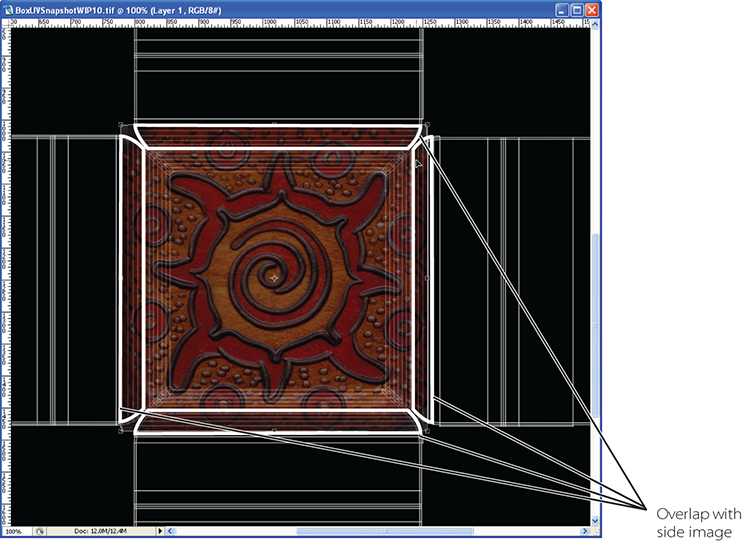
Figure 7-130: Align the right-side image with the right-side UVs.

c07f130.tif
7. Use the same procedures in Photoshop to line up the other sides of the box, as shown in Figure 7-131. Set the box-top image to be the topmost layer, make sure all the layers are at 100% opacity, and then turn off the UV Snapshot layer so it’s not visible.

Figure 7-131: Copy, paste, and line up the box sides and the back to their respective UV areas.

c07f131.eps
8. And finally, open the file boxBottomAndFeet.jpg from the Sourceimages folder of the project. Select the entire image, and copy and paste into your boxColorMap01.psd file. Position and place the image to fit the bottom UVs of the box in your map in Photoshop. Just get close; you will fine-tune the placement of image to UV later.
9. Save the final Photoshop file. Then, resave the file as a JPEG called boxColorMap01.jpg. This is the file you’ll map. (See Figure 7-132.)

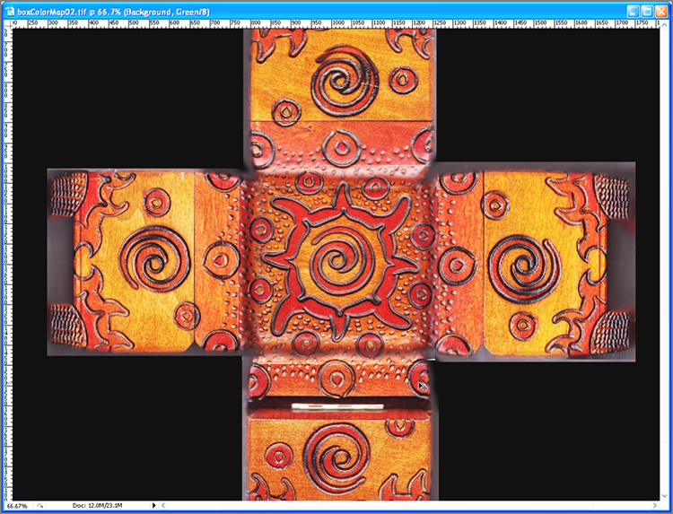
Figure 7-132: The color map layout file boxColorMap01.jpg

c07f132.tif

Mapping the Box

Let’s map this color image to the box and see how it fits. Based on rendering the box, you can make adjustments to the UVs and the image map to get everything to line up. This, of course, requires more Photoshop and/or image-editing experience, which could be a series of books of its own. If you don’t have enough image-editing experience, have no fear: the images have been created for you so you can get the experience of mapping them and learn about the underlying workflow that this sort of texturing requires. Follow these steps:

1. Back in Maya, open the Hypershade window, and create a new Phong shader. Open the Attribute Editor, click the Map icon (c07g003.tif) next to the Color attribute, and select File.
2. Double-click the file1 node to open the Attribute Editor. Click the Folder icon next to the Image Name attribute, navigate to the Sourceimages folder for the project, and select the boxColorMap01.jpg file (not the PSD file). The icon in the Hypershade doesn’t show the image because it’s a large file. (See Figure 7-133.)

Figure 7-133: The color map’s file node

c07f133.tif
3. Double-click the file1 node, and in the Attribute Editor, rename it to boxColorMap. Right-click the newly named boxColorMap node in the Hypershade, and choose Refresh Swatch from the marking menu. The boxColorMap image is displayed as the boxColorMap icon. (See Figure 7-134.)

Figure 7-134: The icon is refreshed.

c07f134.tif
4. Select the box, and assign the Phong shader to it. Rename the Phong to boxShader. In the persp view panel, press 6 for texture view. The color map is fairly well aligned on the model. Not bad! (See Figure 7-135.)

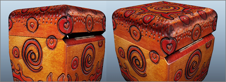
Figure 7-135: The color map fits pretty well already, but there are a few alignment issues at the edges.

c07f135.tif
5. Render a frame to see how the box looks (Figure 7-136). Notice that there are small alignment issues at the edges where the sides meet and where the top meets the sides. Save your Maya scene.

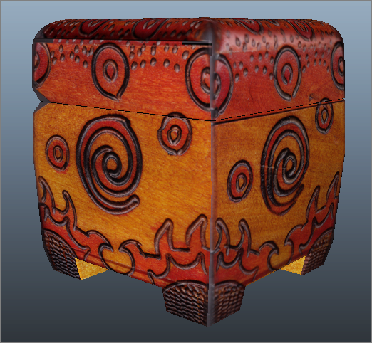
Figure 7-136: A render of the box so far

c07f136.tif

This gives you a pretty good place to work from. You need to adjust the color map image to be more seamless. The scene file boxTexture02.mb in the Scenes folder of the Decorative_Box project on the companion web page will catch you up to this point.

Photoshop Work

This is where image-editing experience is valuable. Here, it’s all about working in Photoshop to further line up the sides to the top and the sides to each other to minimize alignment issues and yield a seamless texture map. Although I won’t get into the minutia of photo editing here, I’ll show the progression of the images and the general workflow used in Photoshop to make the color map’s different sides and top line up or merge better. The images have already been created and are on the companion web page in the Sourceimages folder for this project.

For example, using masking in Photoshop, spend some time feathering the intersection of the box’s sides in boxColorMap01.psd so there is no hard line between the different sides and the top. Figure 7-137 shows a smoother transition between the different parts. This image has been created for you; it’s boxColorMap02.jpg in the Sourceimages folder. Make sure you don’t overwrite that file if you’re painting your own.

Figure 7-137: Use masks to feather the transitions between the different parts of the box.

c07f137.tif

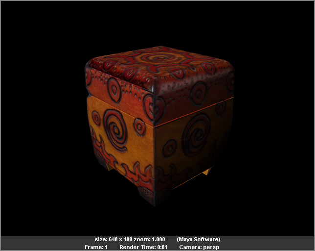
In Maya, double-click the boxColorMap node in the Hypershade, and in the Attribute Editor, replace the original boxColorMap01.jpg with the boxColorMap02.jpg from the Sourceimages folder (or your own retouched image file). Render and compare the difference. The top and front should merge a little better. In the persp view panel, orbit around the box in Texture View mode (press 6) to identify any other lineup issues. In some cases, as you can see in Figure 7-138, gray or black is mapped onto the box on its right side, and there is a warped area. Also, the crease where the lid meets the box is lower than you’ve modeled.

Figure 7-138: There are blank areas on the box as well as a little distortion.

c07f138.tif

The blank areas on the box are outside the bounds of the image in the Photoshop image and can be fixed by adjusting the UVs in Maya. The same goes for the distorted areas on the side of the box—you just need to adjust the UVs.

1. Select the box, and open the UV Texture Editor window. Figure 7-139 shows some primary areas for you to work on.

Figure 7-139: Here are the main problems to fix.

c07f139.eps
2. In the UV Texture Editor, select the UVs (right-click and choose UV) shown in Figure 7-140 on the left. Press W for the Move tool, and realign the UVs to the seam where the lid meets the box, as shown in Figure 7-140 on the right. As you make the changes in the UV Texture Editor, you should immediately notice them in the Perspective window (as long as you’re in Texture View mode).

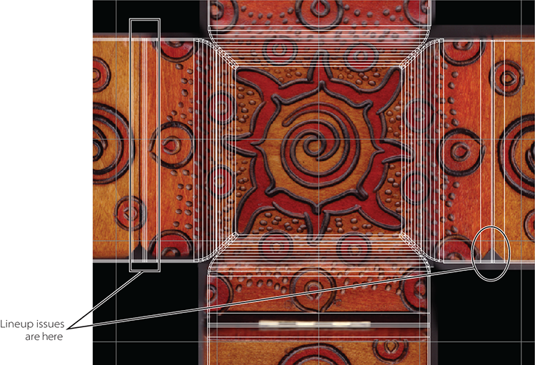
Figure 7-140: Move the UVs.

c07f140.tif
3. Look at the image on top in Figure 7-141. Move the appropriate UVs to align the edge of the UV layout to the image for the right side of the box, as shown on the bottom of Figure 7-141.

Figure 7-141: Line up the UVs to the image for the right side of the box.

c07f141.tif
4. The distortion is getting better, and the texture fits nicer. But notice in the image on the left in Figure 7-142 that the right side of the box and the back of the box don’t line up well. There are some other instances of the textures not lining up well all around the box. Using the Texture view mode (press 6) in the Perspective window and the UV Texture Editor, go around the box in its entirety and adjust the UVs, point by point as needed, so that they all line up to the image in the UV Texture Editor. Make sure that the sides line up at the edges of the box as well as you can. Figure 7-142’s right image shows correctly aligned UVs for the right side/back side of the box. Don’t forget to line up the bottom of the box and feet, too. That part should be much easier.

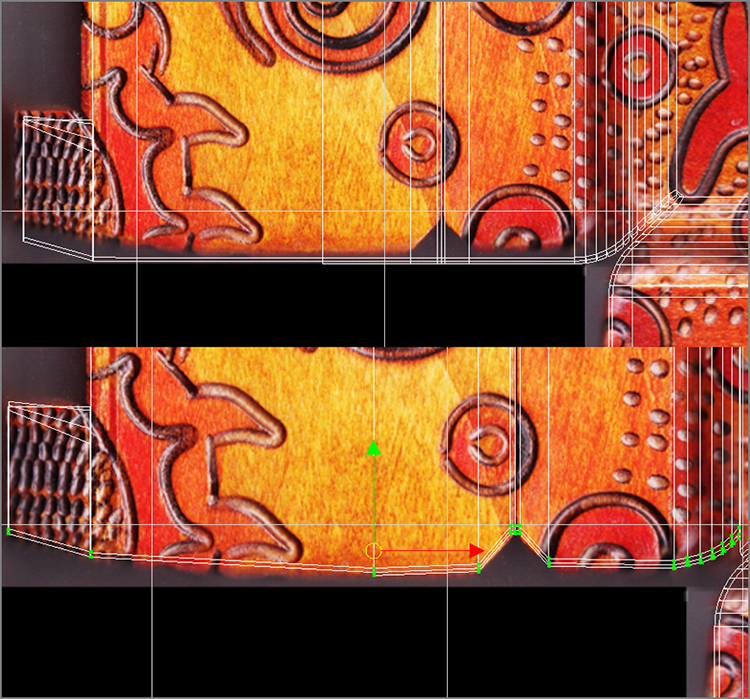
Figure 7-142: Line up the UVs for the right-side/back-side edge of the box.

c07f142.tif

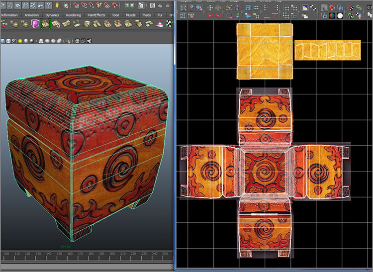
This part of tweaking the UVs takes time and patience. The key is to keep looking back and forth between the UV Texture Editor and the persp panel to see how the textures are lining up as you move the UVs. Figure 7-143 shows the UV Texture Editor and a persp view of the box with UVs lined up and reasonably ready to go. You can compare your work to the scene file boxTexture03.mb in the Scenes folder of the Decorative_Box project on the companion web page. Render a few different views to take in all the hard work. In Chapter 10, you’ll light the box and prepare it for rendering, and in Chapter 11, you’ll use displacement maps created from these photos to detail the indentations and carvings that are in the actual box. You’ve had enough excitement for one chapter.

Figure 7-143: The UVs laid out for the decorative box

c07f143.tif

For Further Study

For a challenge and more experience, create new image maps for the wagon and try your own decal designs. You can even change the textures for the decorative box and make your own design. As previously suggested, you can try to create more realistic wood maps for the wagon’s railings. In Chapter 10, you’ll begin to see how shading and rendering go hand in hand; you’ll adjust many of the shader attributes you created in this chapter to render the decorative box in Chapter 11.

You can also try to create textures to map onto the hand model you created in Chapter 4, using photos of your own hand with extensive UV manipulation.

Summary

In this chapter, you learned about the types of shaders and how they work. Each shader has a set of attributes that give material definition, and each attribute has a different effect on how a model looks.

To gain practice, you textured the table lamp scene using various shaders.

Next, you learned about the methods you can use to project textures onto a surface, and you learned about the Maya texture nodes, including PSD networks and the basics of UVs, and how to use them to place images onto your wagon and decorative box models in detailed exercises exposing you to manipulating UVs and using Photoshop to create maps.

Texturing a scene is never an isolated process. Making textures work involves render settings, lighting, and even geometry manipulation and creation. Your work in this chapter will be expanded in Chapters 10 and 11 with discussions of lighting and rendering.

Just like everything else in Maya, it’s all about collaboration—the more experience you gain, the more you’ll see how everything intertwines.

However, for Maya to be an effective tool for you, it’s important to have a clear understanding of the look you want for your CG. This involves plenty of research into your project, downloading heaps of images to use as references, and a good measure of trial and error.

The single best weapon in your texturing arsenal, and indeed in all aspects of CG art, is your eye, specifically, your observations of the world around you and how they relate to the world you’re creating in CG.

..................Content has been hidden....................

You can't read the all page of ebook, please click here login for view all page.
Reset