One of the first problems you're going to solve in most web applications is authentication. Users will need accounts and they'll need a way to log into those accounts. The way this is done conventionally on the web is by verifying a password.

The worst thing you could do is store the password in a varchar column like any other text. To understand why, you have to think about security and doing that means putting yourself in the shoes of a malicious attacker. You're going to do everything you can to prevent an attacker from gaining access to your database, but good security means ensuring that even if the attacker gets ahold of your database your users' credentials will remain safe. To an attacker, having access to the plaintext passwords would be an incredible win. So you mustn't allow that to happen.

The first step towards better password security is storing a hash value instead of the password. A hash value is just a number generated from text. A cryptographic hash value has two important properties: first, a small change to the input will result in a dramatically different hash value, and second, the input cannot be generated from the hash value. The hash value is one way. So instead of storing the password, we'll store the hash value of the password and when the user tries to authenticate, we'll just check that the password they entered hashes to the same value we have stored from when they set the password. If they match, the user entered the same password. This alone is not sufficient. Imagine if two users use the same password. If you just store the hash value, these two users are going to have the same hash value in the database. Worse, the attacker can generate the hash values for common passwords and go looking through the database for matching. So the next improvement over storing hashes is storing salted hashes. A salt value is just some randomly generated text. If you generate different random text for each user and append it to the password, thanks to the first property of a cryptographic hash algorithm, they'll wind up with dramatically different hashes. The attacker won't be able to simply look for the hashes of common passwords.

One unfortunate property of cryptographic hashes still remains: they're designed for speed. This is great when you're hashing a large document, but when you're dealing with passwords it's not very helpful. You don't want the attacker to be able to check millions of passwords with a particular salt value very rapidly. So ideally you want an algorithm that is computationally expensive.

Thankfully, PostgreSQL comes with an extension that handles all these minutia for you: the pgcrypto module. To install it, run the following SQL in pgAdmin III in the query window as before:

CREATE EXTENSION pgcrypto;

Now let's create a basic users table. For now we'll just have the username and the columns needed to store the password using pgcrypto. In your own applications you'll add other columns to this table, and maybe use other fields instead of a username, such as an account number or an e-mail address, but the same basic ideas will apply.

CREATE TABLE users (
    username varchar,
    password_hash varchar
);

To insert a new user, we must use gen_salt and crypt to generate the requisite values for these columns. Let's see an example, a user bob with password bad password.

INSERT INTO users (username, password_hash)
VALUES ('bob', crypt('bad password', gen_salt('bf')));

You can then authenticate a user by selecting from this table where the usernames match and the supplied password sent through crypt equals the stored hash, like this:

SELECT * FROM users WHERE username = 'bob' and password_hash = crypt('bad password', password_hash);

You'll notice the preceding statement returns bob, but if you use any text other than bad password, you don't:

SELECT * FROM users WHERE username = 'bob' and password_hash = crypt('password', password_hash);

This powerful module contains a number of other convenient functions. It's worth taking a few minutes to browse the documentation and see what else it can do for you. It is always better to use off-the-shelf cryptography code rather than write it yourself. For more information, see http://www.postgresql.org/docs/9.2/static/pgcrypto.html.

One special feature of PostgreSQL that comes in very handy is the RETURNING clause. We've already seen a very basic use of it in creating your first table, so you know you can use it to receive back the row you just inserted or any part of it. This is a handy way to get back the ID value of newly-inserted rows or other information that may be computed by PostgreSQL during insertion. Let's try it with an automatically incrementing integer:

CREATE TABLE bands (
    id SERIAL PRIMARY KEY,
    name VARCHAR,
    inserted_at TIMESTAMP DEFAULT CURRENT_TIMESTAMP
);

INSERT INTO bands (name) 
VALUES ('Led Zeppelin'), ('Andrew W.K.') 
RETURNING *;

PostgreSQL will return the result of the insert as follows:

Result of INSERT with RETURNING

It also works with UPDATE and DELETE, as follows:

UPDATE bands 
SET name = 'Blue Öyster Cult' 
WHERE id = 1 
RETURNING *;

DELETE FROM bands 
WHERE id = 1 
RETURNING *;

These will both return the row with ID 1. The UPDATE will return the row after applying the changes. You aren't limited to RETURNING *, you can use any SQL that goes in the column list of a SELECT statement there, no matter how absurd:

INSERT INTO bands (id, name) 
VALUES (1, 'Led Zeppelin') 
RETURNING id*5, length(name);

In practice, this is mostly used to return the serial ID value, much like MySQL's SELECT LAST_INSERT_ID().

Another contrib module gaining wider use these days is hstore. This module creates a new column type with the same name for storing hash tables or dictionaries of key/value strings. While it is best to design your tables according to relational database theory, there are frequently cases where you don't know ahead of time what columns you'll need to store.

The standard solution to this problem is to create a separate table for the key/value pairs. Suppose we wanted to store arbitrary metadata on posts. The tables might look like this:

CREATE TABLE posts (
    title VARCHAR PRIMARY KEY, 
    content TEXT
);

CREATE TABLE post_metadata (
    title VARCHAR REFERENCES posts, 
    key VARCHAR, 
    value TEXT, 
    PRIMARY KEY (title, key)
);

Now if we wanted to record, say, the author and publication date of the post, we could do that like this:

INSERT INTO posts VALUES ('Hello, World', ''),
INSERT INTO post_metadata (title, key, value) VALUES 
('Hello, World', 'reviewer', 'Daniel Lyons'),
('Hello, World', 'proofread on', '2012-02-21'),

In this case, such a facility might be helpful because we may not want to write a full-fledged review system or we might want to allow a subsystem to store its data in the database without changing the structure of the database.

We can do the same thing with just one table using hstore. First load the hstore extension:

CREATE EXTENSION hstore;

Now let's DROP the old tables and recreate the posts table with an hstore column:

DROP TABLE post_metadata;
DROP TABLE posts;

CREATE TABLE posts (
  title VARCHAR PRIMARY KEY, 
  content TEXT, 
  metadata hstore
);

Now we can proceed to insert the post with the review and proofread metadata directly:

INSERT INTO posts (title, content, metadata) VALUES 
('Hello, world', '', 
   '"reviewer"     => "Daniel Lyons", 
    "proofread on" => "2013-02-21"'),

You can use the -> operator to retrieve a value from the hstore column in a query. For instance, if we wanted to get all the reviewers with the posts they reviewed, we could do this:

SELECT title, metadata->'reviewer' as reviewer 
FROM posts;

If we wanted to recover a table like the post_metadata table from before, we can do that with the function each:

SELECT title, (each(metadata)).key,(each(metadata)).value 
FROM posts;

We can update the metadata using the || operator:

UPDATE posts 
SET metadata = metadata || 
                 '"proofread on" => "2013-02-23"' 
WHERE title = 'Hello, world';

Refer to the online documentation (section F.16 ) for more details about this see http://www.postgresql.org/docs/9.2/static/hstore.html.

It's also perfectly easy to store XML with PostgreSQL. There's a built-in XML type, as well as several built-in functions that permit querying and transformation of XML data. For demonstration, let's create a simple table for storing HTML documents and put a couple of sample documents into it:

CREATE TABLE documents (
    doc xml,
    CONSTRAINT doc_is_valid CHECK(doc IS DOCUMENT)
);

The xml type itself permits invalid data, so we've added a constraint to ensure that the XML in the doc column will always be well-formed. Let's add a simple HTML document.

INSERT INTO documents VALUES (
'<html>
<head><title>Hello world</title></head>
<body><h1>First heading</h1></body>
</html>'),

We can use the xpath function to retrieve parts of XML documents. XPath is a small language for accessing parts of XML documents. The basic syntax is tag names separated by slashes much like a filesystem path. Let's see an example query:

SELECT 
    (xpath('//title/text()', doc))[1]::varchar AS title,   
    (xpath('//h1/text()', doc))[1]::varchar AS h1 
FROM documents;

The result of this query will look like this:

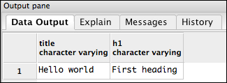
The syntax of the xpath function is xpath(path, document). Our path queries look very similar to each other: //title/text(), which means approximately find the text within the <title> element wherever it occurs. The XPath queries can always return multiple values, so we're using the array subscript syntax to obtain just the first result, which is why both columns look like (xpath(path, doc))[1]. Finally, we cast the result to a varchar value with the column::type syntax and name the column with the AS syntax. There's a lot going on in there, but we're getting exactly what we want out.

We can make this query a little simpler to run by defining a function as follows:

CREATE FUNCTION document_title(xml) RETURNS varchar AS $$ SELECT (xpath('//title/text()', $1))[1]::varchar
$$ LANGUAGE 'sql';

Now we can do the query a little more simply:

SELECT document_title(doc) from documents;

We can even do fancier tricks with this, such as indexing on the title:

CREATE INDEX document_title_index 
ON documents (document_title(doc) varchar_pattern_ops);

The varchar_pattern_ops code indicates to PostgreSQL that you want to perform LIKE queries against this index. This will make it possible for queries like this to be executed against this index:

SELECT * FROM documents 
WHERE document_title(doc) LIKE 'Hello%';

Bear in mind that until the table becomes large PostgreSQL will prefer sequential scans. This is one reason it's essential to test with data similar in size and shape to production data.

XML is one solution to dealing with hierarchical data, but it isn't the most natural for the relational database. Instead, you often wind up with nested categories, or filesystem-like folder hierarchies, or links back to older records. A popular way to structure a relational database for data with this shape is using a self reference, a link back to a parent object in the same table. For instance, you might want to model categories that can have subcategories with arbitrary nesting. A simple table might look like this:

CREATE TABLE categories (
    id SERIAL PRIMARY KEY,
    name VARCHAR,
    parent_id INTEGER REFERENCES categories
);

What makes this structure recursive is that self-referencing parent_id column, which refers to the table we're defining from within its own definition. We would treat categories with a NULL value for the parent_id column as top-level categories, categories that do not belong within any other category.

To get a feel for the kind of data, let's put a few categories in there for an online retailer. Say we sell shirts and books, and books we further divide into fiction and non-fiction, and then we'll put programming books inside non-fiction. It might look like the following:

INSERT INTO categories (id, name, parent_id) VALUES
(1, 'Shirts', NULL),
(2, 'Books', NULL),
(3, 'Fiction', 2),
(4, 'Non-fiction', 2),
(5, 'Programming', 4);

Usually you won't put these in manually like this, but you can see that Fiction and Non-fiction are children of the Books category because their parent_id values are 2, the value for Books is NULL and Programming has the parent_id value as 4, which is the id value for Non-fiction.

Suppose you want to make navigation breadcrumbs given a category. You need to look up that category and then you need to look up the parent category. You need to do this until the parent category is NULL. In a procedural pseudocode, the process might look like the following:

def write_breadcrumbs(category):
    row = getOne("SELECT * FROM categories 
                  WHERE id = ?", category)

    while row['parent_id'] != NULL:
        write(row['name'])
        write(' > ')

        row = getOne("SELECT * FROM categories 
                      WHERE id = ?", row['parent_id'])

This kind of solution leads to the N+1 query problem. There's an action you want to take for a particular value, but to take that action you have to run an arbitrary number of separate queries. Recursive queries in PostgreSQL provide you with a way to have the database do the heavy lifting instead. Because we'll be using recursion in the SQL, let's first see what a recursion formulation would look like in our pseudocode:

def write_breadcrumbs(category):
    row = getOne("SELECT * FROM categories 
                  WHERE id = ?", category)
    write(row['name'])
    if row['parent_id'] != NULL:
        write(' > ')
        write_breadcrumbs(row['parent_id'])

It's debatable whether this is better code; it's shorter, and it has fewer bugs, but it also might expose the developer to the possibility of stack overflows. Recursive functions always have some similar structure though, some number of base cases that do not call the function recursively and some number of inductive cases that work by calling the same function again on slightly different data. The final destination will be one of the base cases. The inductive cases will peel off a small piece of the problem and solve it, then delegate the rest of the work to an invocation of the same function.

PostgreSQL's recursive query support works with something called the common table expressions (CTEs). The idea is to make a named alias for a query. We won't delve into the details too much here, but all recursive queries will have the same basic structure:

WITH RECURSIVE recursive-query-name AS (
    SELECT <base-case> FROM table
    UNION ALL
    SELECT <inductive-case> FROM table 
    JOIN <recursive-query-name> ON )
SELECT * FROM <recursive-query-name>;

For an example, let's get all the categories above Programming. The base case will be the Programming category itself. The inductive case will be to find the parent of a category we've already seen:

WITH RECURSIVE programming_parents AS (
    SELECT * FROM categories WHERE id = 5
    UNION ALL
    SELECT categories.* FROM categories 
    JOIN programming_parents ON 
         programming_parents.parent_id = categories.id)
SELECT * FROM programming_parents;

This works as we'd hope:

Output of a simple recursive query

Without using this trick we'd have to do three separate queries to get this information, but with the trick it will always take one query no matter how deeply nested the categories are.

We can also go in the other direction and build up something like a tree underneath a category by searching for categories that have a category we've already seen as a parent category. We can make the hierarchy more explicit by building up a path as we go:

WITH RECURSIVE all_categories AS (
    SELECT *, name as path FROM categories WHERE parent_id IS NULL
    UNION ALL
    SELECT c.*, p.path || '/' || c.name 
    FROM categories AS c 
    JOIN all_categories p ON p.id = c.parent_id)
SELECT * FROM all_categories;

Finding all the categories with their path

We can be more discriminating with the search by looking for a particular category as the starting value in the base case:

WITH RECURSIVE all_categories AS (
    SELECT *, name as path FROM categories WHERE id = 2
    UNION ALL
    SELECT c.*, p.path || '/' || c.name 
    FROM categories AS c 
    JOIN all_categories p ON p.id = c.parent_id)
SELECT * FROM all_categories;

The category tree rooted at Books

This is hugely useful with hierarchical data.

Often you will have large text documents in your database and want to search for documents by their content. If your documents are small and your table has few rows, the ordinary LIKE queries are sufficient, but once your documents get bigger or you want relevance ranking, you will start to want a better solution. For this, PostgreSQL has built-in support for full-text searching. Let's make a simple table and test it out:

CREATE TABLE posts (
    title varchar primary key,
    content text
);

INSERT INTO posts (title, content) VALUES
('Hello, world', 'This is a test of full-text searching!'),
('Greetings', 'Posts could be blog articles, or ads 
or anything else.'),

Now a basic non-full-text search would be to use the LIKE operator, which could look like this:

SELECT title FROM posts WHERE content LIKE '%article%';

This will return the second row's title, Greetings. This approach is nice, but very limited, after all, if we had used %post% nothing would have been returned because of a difference in case.

The text search facility is a bit more complex. Before the search can be performed we have to convert the document into tsvector and the query into tsquery. Then we must use the @@ operator to perform a tsquery against a tsvector.

We can convert text into tsvector using the to_tsvector function and we can convert a query into tsquery using plainto_tsquery like so:

SELECT title FROM posts 
WHERE to_tsvector(content) @@ plainto_tsquery('post'),

This query will return the second row, because under the covers to_tsvector does more than change the types, it also normalizes the text by removing suffixes such as '-s' and '-ing'. Along similar lines, plainto_tsquery does more than converting a string into a query, it also insinuates some special operators that the full-text search system can understand, translating a string like 'blog posts' into 'blog & post', which will only match documents that possess both words. If you want to use the extended search language directly, you can do so, just use to_tsquery instead, and refer to section 8.11.2 of the PostgreSQL manual, which describes the text search operators &, |, and !, at http://www.postgresql.org/docs/9.2/static/datatype-textsearch.html#DATATYPE-TSQUERY.

As nice as this is, it's pretty inefficient, because PostgreSQL isn't using any indexes on this data, so it must regenerate tsvector for each row, on every select. We can speed things up considerably by indexing tsvector:

CREATE INDEX posts_content_search_index ON posts
USING gin(to_tsvector('english', content));

The english argument there tells us to_tsvector what language we want it to use. gin is a type of index (Generalized Inverted Index (GIN)). The manual details when you would choose GIN and when you would choose Generalized Search Table (GIST)indexes, but the rule of thumb for text search is that documents, which are read more often than written should use GIN indexes while frequently-updated documents should use GIST.

Now that we have this index in place, performing full text searches becomes very efficient. Next, one might want to know something about the quality of the search results. You can find out by using the ts_rank or ts_rank_cd functions:

SELECT title, ts_rank_cd(to_tsvector(content), query)
FROM posts, plainto_tsquery('post') AS query
WHERE to_tsvector('english', content) @@ query
ORDER BY ts_rank_cd(to_tsvector(content), query)

The result here shows that we have a rank code of 0.1, which is low, but with such simple documents it's unlikely we could get it to be higher.

One more improvement would be to use the title in the vector, and give it a weight to reflect its greater importance. You can construct such vectors quite easily, though the syntax is somewhat odd: setweight(tsvector, char). This function assigns a weight to the enclosed tsvector. To make good use of it, we have to combine several tsvectors with different weights. The regular string concatenation operator || lets us do exactly that. Let's see it in action by recreating the index, this time including the title and assigning the title and document different weights:

DROP INDEX posts_content_search_index;
CREATE INDEX posts_content_search_index ON posts 
USING gin((setweight(to_tsvector('english', title), 'A')
      ||(setweight(to_tsvector('english', content), 'B'))
));

We've decided to give the title value a weight of A, the highest, and the content B, the second highest. In practice you might have other levels for tags or keywords, the author, the category, or whatever else you might imagine. If we were indexing a products table, the product name could be weight A, the manufacturer could be weight B, keywords weight C, and the description or reviews weight D. It's up to you to decide what the different levels are. The available levels are A through D.

These nested functions are getting unwieldy to write, so let's make a view to simplify things for us:

CREATE VIEW posts_fts AS 
SELECT *,
  setweight(to_tsvector('english', title), 'A') || 
  setweight(to_tsvector('english', content), 'B') 
    as vector
FROM posts 

Now we can make the query look a lot tidier:

SELECT title, ts_rank_cd(vector, query)
FROM posts_fts, plainto_tsquery('hello') as query
WHERE vector @@ query

Also, notice the rank has gone from 0.1 to 1, because hello is in the title value, which has rank A.

It's important to be comfortable with database backup and restore procedures. The only way to conquer nerves about these procedures is to do them frequently enough that they become second nature. I'm going to show you how to do these tasks through pgAdmin III on your desktop and I'll include the command-line equivalents so that you can see how to perform these tasks in a headless Unix server environment.

If you've been following along there should be some tables with a small amount of data in them on your server.

In pgAdmin III, right-click on the database and select Backup…:

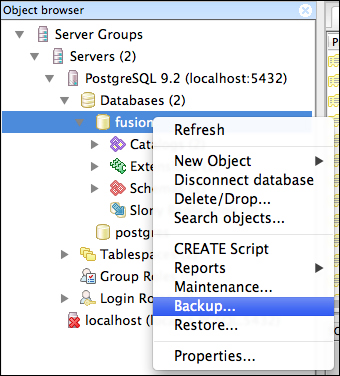
The backup menu item

You'll see a new window appear as follows:

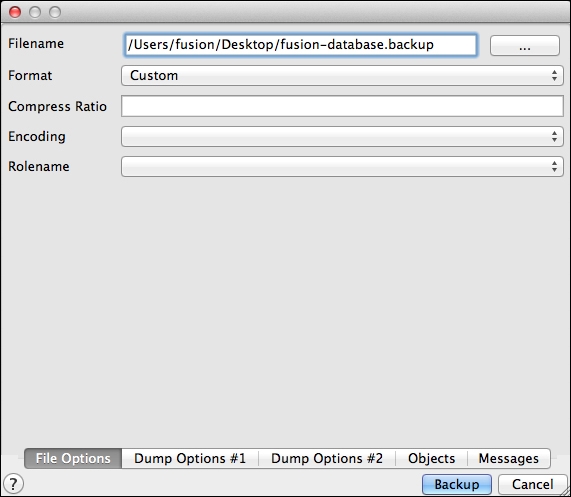
The backup configuration dialog

As I've done, choose the Custom value in Format and ensure that your filename ends in .backup and then click Backup. The dialog will change into this:

Output from pg_dump

The key here is the last line: Process returned exit code 0. If you get a different response, read through the dialog and see what happened, chances are, you ran out of disk space. Otherwise the backup worked fine and you have the entire contents of that database in a file that can be loaded back into this or any other PostgreSQL server (assuming it is the same version or newer).

Now let's delete this database and re-create it. Right-click on the database name and choose Delete/Drop…. It will prompt you to proceed. Go ahead and delete the database, then create a new one by right-clicking on the databases icon in the tree. All you have to supply is the name.

Now right-click on the database in the tree and choose Restore…:

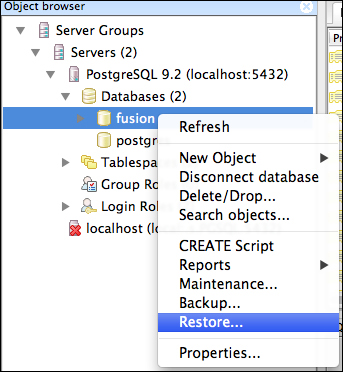
The Restore… command

All you should need to specify in the dialog is the path to the backup file, as follows:

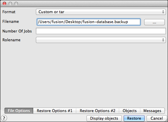
The restore configuration dialog

Proceed with the restore and you should get similar output to the backup, again ending in Process returned exit code 0 as follows:

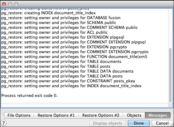
Output from pg_restore

That's it, you've backed up and restored your database.

From Unix, what you've just done is equivalent to this sequence of commands:

$ pg_dump -Fc -f fusion-database.backup -U fusion fusion 
$ dropdb fusion 
$ createdb -O fusion fusion
$ pg_restore -d fusion fusion-backup.backup

One question you're bound to ask yourself sooner or later is, how big are these tables? PostgreSQL has some convenient functions you can use to find out just how big various things are in the backend. For instance, to see the total size of a database, you can run pg_database_size. I have wrapped all these examples with pg_size_pretty, which takes a number of bytes and returns a human-friendly string with appropriate units (kilobytes, megabytes, and so on):

SELECT pg_size_pretty(pg_database_size('fusion'));

This returned 6629 KB for me. To see just the size of a table, you can run:

SELECT pg_size_pretty(pg_relation_size('posts'));

This returned just 4 KB for me. Note that this is just the raw table size and doesn't include indexes. To get the whole picture, use pg_total_relation_size:

SELECT pg_size_pretty(pg_total_relation_size('posts'));

This returned 32 KB, a marked increase in size just from including indexes. Keeping your index sizes reasonable is a big part of database administration. The trick is choosing columns to index by knowing which queries need to be optimized. There's a lot of literature on the subject, but one of the best ways to learn more is to read Markus Winand's excellent tutorial on the subject, Use the Index, Luke! at http://use-the-index-luke.com/.

PostgreSQL provides quite a few helpful built-in functions like these. See section 9.26. System Administration Functions of the documentation for more: http://www.postgresql.org/docs/9.2/static/functions-admin.html.

One of the most amazing things about relational databases is what goes on under the hood when you perform a query. In broad strokes, the database first parses the query, checks to make sure it is sensible, and then dreams up many different ways to perform the query. It then ranks these query plans according to estimated cost and chooses the cheapest one to perform. This process is happening transparently with every query you issue. So what do you do when you realize a query is performing poorly?

The answer is to put EXPLAIN at the start of your SELECT statement. This tells PostgreSQL that rather than executing your query you want it to tell you what it would do in order to execute it. If you use EXPLAIN ANALYZE instead it will also run the query and include actual timing data. Let's run the following query on our posts table and see what happens:

EXPLAIN ANALYZE SELECT * FROM posts;

PostgreSQL responds with the following text:

 Seq Scan on posts  (cost=0.00..16.40 rows=640 width=96) (actual time=21.817..21.819 rows=1 loops=1)
 Total runtime: 21.883 ms

This is not a very interesting query, but you can see PostgreSQL has told us that it's going to use a sequential scan on the table. Depending on the size of the table and whether or not it is cached in memory this may or may not be a problem, but without looking for specific values it would be hard to optimize. Let's get a more interesting query plan using one of our recursive queries:

EXPLAIN ANALYZE
WITH RECURSIVE all_categories AS (
    SELECT *, name as path FROM categories WHERE id = 2
    UNION ALL
    SELECT c.*, p.path || '/' || c.name 
    FROM categories AS c 
    JOIN all_categories p ON p.id = c.parent_id)
SELECT * FROM all_categories;

The query plan we get back looks like this:

 CTE Scan on all_categories  (cost=291.34..302.96 rows=581 width=72) (actual time=24.356..24.600 rows=4 loops=1)
    CTE all_categories
        ->  Recursive Union  (cost=0.00..291.34 rows=581 width=72) (actual time=24.350..24.585 rows=4 loops=1)
            ->  Index Scan using categories_pkey on categories  (cost=0.00..8.27 rows=1 width=40) (actual time=24.344..24.347 rows=1 loops=1)
                Index Cond: (id = 2)
                ->  Subquery Scan on "*SELECT* 2"  (cost=0.33..27.72 rows=58 width=72) (actual time=0.062..0.066 rows=1 loops=3)
                ->  Hash Join  (cost=0.33..27.14 rows=58 width=72) (actual time=0.056..0.059 rows=1 loops=3)
                    Hash Cond: (c.parent_id = p.id)
                    ->  Seq Scan on categories c  (cost=0.00..21.60 rows=1160 width=40) (actual time=0.005..0.007 rows=5 loops=3)
                        ->  Hash  (cost=0.20..0.20 rows=10 width=36) (actual time=0.008..0.008 rows=1 loops=3)
                        Buckets: 1024  Batches: 1  Memory Usage: 1kB
                        ->  WorkTable Scan on all_categories p  (cost=0.00..0.20 rows=10 width=36) (actual time=0.002..0.003 rows=1 loops=3)
                         Total runtime: 24.758 ms

Despite the complexity of the plan, it's still executing pretty quickly. Note that a complex plan isn't necessarily a bad thing. If you are doing searches for particular values and seeing both a performance problem and sequential scan, it probably means you're missing an index, but the query plan will probably be very simple. In this case, the performance probably has more to do with the table being small enough to fit in memory.

One the most important things to know about optimizing database performance is that the database will behave differently depending on its configuration and the size of the tables being queried. You may have tables with the same structure on your machine and on production, but if your production database has 4 gigabytes of data in this table and your laptop has 10 megabytes, you might see radically different query plans. It's essential when debugging database performance problems that your databases be configured as close to identical as possible and have as close to identical data. Different hardware, different configuration files, different versions of PostgreSQL, or different data can all cause large differences in performance.

If you want to know more about PostgreSQL performance optimization with the EXPLAIN statement, consult section 14.1. Usi ng EXPLAIN of the official PostgreSQL documentation, available here at http://www.postgresql.org/docs/9.2/static/using-explain.html.