
8
A Study of WSN Privacy Through AI Technique
Piyush Raja
Department of CSE, COER University, Roorkee, India
Abstract
Wireless sensor network (WSN) collects data then interpret the informations about the environment or the object they are sensing. Owing to the energy and the bandwidth limit, those sensor usually has reduced communication capability. WSN keep track of changing conditions in real time. External variables or the device designers themselves are to blame for this complex behaviour. Sensor networks often use deep learning methods to respond to certain situations, avoiding the need for wasteful overhaul. Machine learning also inspires plenty of realistic strategies for maximising resource use and extending the network’s lifetime. We included a comparison guide in this paper to assist WSN designers in designing appropriate machine learning (ML) strategies for their unique implementation problems.
WSN (Wireless Sensor Network) are gaining popularity among researchers. One of the most important problems is to preserve their privacy. This region has received a significant amount of attention in recent years. Surveys and literature studies have also been conducted to provide a comprehensive overview of the various techniques. However, no previous research has focused on privacy models, or the set of assumptions utilised to construct the method. This work, in particular, focuses on this topic by reviewing 41 studies over the previous five years. We call attention to the significant variances that exist across linked studies, which might make them incompatible if used at the same time. We present a set of recommendations for developing comprehensive privacy models in order to facilitate comparison and appropriateness analysis for various circumstances.
Keywords: WSN, supervised learning, unsupervised learning, reinforcement learning
8.1 Introduction
A wireless sensor network (WSN) is made up of a number of self-contained, small, low-cost, and low-power sensor nodes. These nodes collect information about their surroundings and work together to send it to centralised backend units known as base stations or sinks for further analysis. Sensor nodes could be fitted with thermal, acoustic, chemical, pressure, weather, and optical sensors, among others. WSNs have a lot of capacity for designing powerful applications because of their diversity. Each one has its own set of characteristics and criteria. It’s a difficult challenge to create powerful algorithms that can be used in a variety of applications. WSN programmers must solve concerns such as data collection, data reliability, translation, node clustering, energy conscious routing, events scheduling, fault identification, and protection in particular. Machine learning (ML) was first used in the late 1950s as an artificial intelligence tool (AI) [1]. Its emphasis changed over time, focusing more on algorithms that are computationally feasible and stable. The extensive availability of networks in modern cultures, as well as the growth of linked gadgets that people use on a daily basis, emphasises the pervasiveness of today’s information technology.
Wireless communications, such as cellular networks, rely on technology or communication equipment deployment that is planned ahead of time. However, due to present sophisticated cellular network applications, infrastructure in many locations is unreachable (i.e. earthquake hit-places, violent regions, battlefields, volcanic prone areas). Self-organization, infrastructure-free independence, flexibility, and cost savings have all grown in popularity. A Wireless Sensor Network (WSN) is the only solution to solve these problems in the example above, such as sending communications between nodes without a structure. This network also creates the possibility of a novel way for acquiring and retrieving data from the monitored area. We were inspired to work in this neighborhood by these wonderful homes.
The design and development of small wireless devices, such as sensors, capable of sensing, processing, computing, and networking, also benefited technical achievements [2]. WSNs are often made up Dozens and dozens of devices are scattered over hard terrain at irregular intervals or condition” in a defined keypoint. They are used for a number of things. During either deployment, which is a typical option, sensors are produced in an ad-hoc fashion to shape the network. Contact is formed by single-hop or multi-hop propagation, depending on the sensors. As a consequence, WSNs have piqued the scientific community’s attention due to their wide range of applications, including military applications, fire detection, health and environmental protection, and habitat monitoring. Sensors are tiny computers with limited resources, such as memory, processors that are relatively slow, or resource-constrained transceivers. For certain applications, neither method is viable, particularly when sensors are widely spread or situated in remote places where human intervention is prohibited. As a consequence, one of the most difficult difficulties in WSNs is energy conservation, which is viewed as a vital component in the network’s long-term sustainability. As a consequence, several algorithms and strategies have been suggested and developed from various viewpoints in order to make better use of this restricted energy budget and prolong the lifetime and operation of these devices as much as possible. In WSNs with tree topologies, data collecting is one of the most important activities. To accomplish an implementation objective, each of these sensors may detect the monitoring area and transfer data to a collecting site known as a sink or base station. After receiving the data, the sink makes an appropriate decision based on the application’s requirements. The sink is a critical node that receives all data and connects the WSN to the outside world. Furthermore, WSNs establish a natural many-to-one traffic paradigm by reporting data from sensors to the sink.
This paper’s purpose is somewhat different from previous ones. Rather of focusing on the methodologies used, this study focuses on the models that were explored. Models are made up of all of the assumptions that have been made about the system. Three primary sets of decisions may be recognised in a WSN situation. First, broad concerns such as objectives and dangers must be stated. After then, the network’s intended operation must be defined. Finally, the capabilities and resources of the adversary must be defined. It should be emphasised that if separate contributions rely on distinct models, they may not operate well together. As a result, it’s necessary to have a comprehensive picture of the models under consideration in order to determine whether two or more processes are compatible. In Figure 8.1a shows the architecture of wireless sensor networks and Figure 8.1b shows the Scheme of the Wireless sensor networks (WSNs).
The following are the key reasons why machine learning is critical in WSN applications:
- Sensor networks are typically used to track complex conditions that change rapidly. For example, soil erosion or sea turbulence can cause a node’s position to shift. Sensor networks that can adapt and run effectively in such environments are desirable [7].

Figure 8.1 (a) Architecture of wireless sensor network (WSN). (b) Scheme of the WSNs.
- In exploratory uses, WSNs may be used to gather new information about inaccessible, hazardous sites (e.g., volcanic eruptions and waste water monitoring). System designers may create solutions that initially do not work as intended due to the unpredictable behaviour trends that may occur in such scenarios.
- WSNs are typically used in complex systems where researchers are unable to create precise statistical models to explain machine behaviour. And in the meantime, while some Wireless sensor tasks can be predicted using simple mathematical equations, others can necessitate the use of complex algorithms (for instance, the routing problem). Machine learning offers low-complexity predictions for the system model in related situations.
8.2 Review of Literature
The nodes switch from one x-y coordinate location to another with a separate x-y coordinate. The node’s movement leaves them vulnerable to attack and it’s easy to attack and vanish if they can move. Attacks are also intelligent, acting individually in various scenarios. As a result, the table above outlines the standard approaches for solving problems in WSN. The basic principles connected to WSN are introduced in this section. Following that, a brief description of the papers included in this survey is provided. They are categorised in particular based on the methodology used. This allows for the display of the variety of methodologies used, demonstrating the importance of the survey. A WSN is made up of a collection of sensors that are connected in an ad hoc manner. Sensors are commonly thought to have limited and nonremovable battery storage. Their interconnection is typically ad hoc, necessitating decentralised coordination. As a result, nodes share information and perform processing tasks in a distributed manner. A WSN generally has four entities in addition to sensors (Figure 8.2). The server, or sink, is the node that collects sensory data on the one hand. This information may reach the sink either through direct route (straight lines in Figure 8.2) or through specific sensors that collect data from nearby ones, as will be discussed later (dotted lines in Figure 8.2). The presence of a user is also assumed in order to access the network. Finally, Trusted Third Parties (TTPs) may be considered for credential management and dispute resolution, among other things [13]. These networks have been used in a variety of applications and situations with great success. Akyildiz presented a broad range of situations, ranging from military (e.g., reconnaissance) to environmental (e.g., animal tracking) to domestic (e.g., surveillance) (e.g., smart environments). Researchers have also looked at the security risks surrounding their use in automated manufacturing in recent years. The collection of articles under consideration is divided into sections that focus on distinct aspects of privacy protection. This section examines the methods used on each project. In Table 8.1, it shows that different authors use different methods, routing protocols, showing problem formulation matrices.

Figure 8.2 The NN architectute.
Table 8.1 Literature review.
| Authors | Routing protocols | Methods | Problems formulation metrics | |
|---|---|---|---|---|
| Kannan et al. | Secure AODV routing protocol | MANET | Security problem | Accuracy |
| Nakayma et al. | Trusted AODV | MANET | Attack prevention | PDF, AT, AED, NRL. |
| Boukerche et al. | AODV | MANET | Routing problem | Accuracy |
| W. Wu et al. | AODV | MANET | Routing protocol efficiency | Accuracy |
| Parma Nand et al. | DSR | Qualnet | Routing | Number of hops per route |
| Samir et al. | DSR | MANET | Mobile pattern analysis | Accuracy |
| Chetna et al. | AODV | NS2 | Black hole detection | Efficiency |
8.3 ML in WSNs
Machine learning (ML), a branch of artificial intelligence (AI), is the branch of computer science that is concerned with the analysis and interpretation of routines and procedures in technology to facilitate learning, reasoning, and decision-making without the involvement of a person. Simply defined, machine learning enables users to send massive amounts of data into computer algorithms, which then evaluate, recommend, and decide using just the supplied data. The algorithm can use the knowledge to enhance its judgement in the hereafter if any adjustments are found.
Machine learning is typically described by sensor network designers as a set of tools and algorithms that are used to construct prediction models. Machine learning researchers, on the other hand, see it as a vast space with many themes and trends. Those who want to add machine learning to WSNs should be aware of such themes. Machine learning algorithms, when used in a variety of WSNs implementations, have immense versatility. This section discusses some of the theoretical principles and techniques for implementing machine learning in WSNs. The intended structure of the model can be used to categorise existing machine learning algorithms. The three types of machine learning algorithms are supervised, unsupervised, and reinforcement learning [3].
All businesses depend on data to function. Making decisions based on data-driven insights might be the difference between staying competitive or falling farther behind. In order to harness the value of corporate and customer data and make decisions that keep a business ahead of the competition, machine learning may be the answer.
Despite the efforts of Minimal power supplies continue to be an important barrier with WSNs, especially since they are located in hostile settings or in remote locations, according to the academic researchers are widely dispersed; battery replacement or replenishment is impossible, so energy should be used efficiently to extend their life as much as possible. It’s also challenging to figure out their topology [12]. Due to node failure, the topology is more likely to change after installation and topology formation. Reconstructing topology might also help you conserve electricity. Another significant challenge for WSNs is the creation of an energy-saving tour for deployed static sensors. Another important stumbling block for WSNs is poor memory. Because the sensor nodes are small computers with limited memory and operate on batteries, their data collection process must be reliable to prevent buffer overflow. The study’s main goal is to develop WSNs that use a low-cost energy-saving technology. In order to do so, this research looks at two major concerns. According to the literature evaluation, there is a research gap for idle listening state and sink versatility with single-hop contact.
8.3.1 Supervised Learning
Learning by training a model on labelled data is referred to as supervised learning. It’s a very common method for predicting a result. Let’s say we want to know who is most likely to open an email we send. We can use the information from previous emails, as well as the “label” that indicates whether or not the recipient opened the email. We can then create a training data set with information about the recipient (such as location, demographics, and previous email engagement behaviour), as well as the label [4]. Our model learns by experimenting with a variety of methods for predicting the label based on the other data points until it discovers the best one. Now we can use that model to predict who will open our next email campaign. Figure 8.3 shows the smartness of machines due to ML.

Figure 8.3 Machine learning (Source - Google).
The process of providing input data as well as correct output data to the machine learning model is known as supervised learning. A supervised learning algorithm’s goal is to find a mapping function that will map the input variable(x) to the output variable(y). Supervised learning can be used in the real world for things like risk assessment, image classification, fraud detection, spam filtering, and so on.
What is the Process of Supervised Learning?
Models are trained using a labelled dataset in supervised learning, where the model learns about each type of data. The model is tested on test data (a subset of the training set) after the training process is completed, and it then predicts the output [3]. Figure 8.4 will help you understand how supervised learning works:

Figure 8.4 Supervised learning.
Assume we have a dataset with a variety of shapes, such as squares, rectangles, triangles, and polygons. The model must now be trained for each shape as the first step.
A labelled training set (i.e., predefined inputs and established outputs) is used to construct a machine model in supervised learning. Easy modules that operate in parallel make up neural networks. The biochemical nervous system stimulates these elements. Connections among various components, by their very existence, identify unique network functions. By changing the values of the weights (connections) among several components, a person could easily train a NN to perform a specific purpose. In certain cases, neural networks are conditioned or modified such that feedback leads to a certain target output [5]. In certain cases, neural networks are conditioned or modified such that feedback leads to a certain target output. The following diagram depicts such a situation. If the network O/P equals the real target, the network is settled upon at this stage, based on a calculation of the O/P in addition to the target. In order to train a network, certain input/target pairs are usually necessary. ‘Learning’ is a supervised process that occurs for any single loop or’epoch’ that is illustrated with a novel input pattern by a forward activation flow of O/Ps, in addition to backwards error propagation of weight amendments, according to this law, as it is for other types of backpropagation techniques.
In general, a neural network is illustrated for a given scheme, which allows an arbitrary ‘guess’ as to what it may be. These networks have been programmed to carry out complex tasks in a variety of areas, including voice, pattern recognition, vision, control systems, detection, and classification. Neural networks may also be programmed to solve problems that are difficult for traditional computers or humans to solve [14]. Despite the fact that neural networks use a variety of learning principles, this demonstration focuses solely on the delta law. The most general class of Artificial Neural Networks known as feed forward neural networks often employs this particular delta law. The NN teaching requirements are summarised as follows:
- Feedback neurons receive input.
- The output response obtained is compared to the input data.
- The weights attached to neurons are managed using error data.
- During the back signal, hidden units discover their mistake.
- Finally, the weights are changed.
8.3.2 Unsupervised Learning
Unsupervised learning does not require labelled data, unlike supervised learning. In its place, theypursue to disclose unseen outlines besides associations to theit datas. When we don’t know exactly what we’re looking for, this is ideal. Clustering algorithms, the most common example of unsupervised learning, take a large set of data points and find groups within them. For example, let’s say we want to divide our customers into groups, but we’re not sure how to do so. They can be found using clustering algorithms.
Labels are not offered to unsupervised learners (i.e., there is no output vector). Principal component analysis (PCA) is a well-known technique for compressing higher-dimensional data sets to lower-dimensional data sets for data analysis, apparition, feature extraction, or compression. After mean centering the data for each attribute, PCA requires calculating the Eigen value decomposition of a data covariance medium or singular value decay of a data matrix.
Because unlike supervised learning, we have the input data but no corresponding output data, unsupervised learning cannot be used to solve a regression or classification issue directly. Finding the underlying structure of a dataset, classifying the data into groups based on similarities, and representing the dataset in a compressed manner are the objectives of unsupervised learning.
Example: Let’s say a dataset including photos of various breeds of cats and dogs is sent to the unsupervised learning algorithm. The algorithm is never trained on the provided dataset, thus it has no knowledge of its characteristics [6]. The unsupervised learning algorithm’s job is to let the picture characteristics speak for themselves. This operation will be carried out using an unsupervised learning method by clustering the picture collection into the groupings based on visual similarity.
The following are a few key arguments for the significance of unsupervised learning:
- Finding valuable insights from the data is made easier with the aid of unsupervised learning.
- Unsupervised learning is considerably more like how humans learn to think via their own experiences, which brings it closer to actual artificial intelligence.
- Unsupervised learning is more significant since it operates on unlabeled and unordered data.
- Unsupervised learning is necessary to address situations where we do not always have input data and the matching output.
Unsupervised Learning Benefits
Compared to supervised learning, unsupervised learning is employed for problems that are more complicated since it lacks labelled input data.
Unsupervised learning is preferred because unlabeled data is simpler to get than labelled data.
Unsupervised Learning Drawbacks
Due to the lack of a comparable output, unsupervised learning is inherently more challenging than supervised learning.
As the input data is not labelled and the algorithms do not know the precise output in advance, the outcome of the unsupervised learning method may be less accurate. Figure 8.5 shows how that it works.

Figure 8.5 Unsupervised learning (Source - Google).
The following are the steps that are usually followed when doing PCA:
- Step 1: Get data from the iris regions that has been normalised. By concatenating each row (or column) into a long vector, a 2-D iris image may be represented as a 1-D vector.
- Step 2: From each image vector, subtract the mean image. The average should be calculated row by row.
- Step 3: Compute the covariance matrix to get the eigen vectors and eigen values.
- Step 4: Examine the covariance matrix’s eigenvectors and Eigen values.
- Step 5: The eigenvectors are sorted according to their Eigen values, from high to low. Forming a function vector by selecting elements.
- Step 6: Build a new data set We basically take the transpose of the vector and increase it on the left of the initial data set, transposed, until we’ve selected the components.
Final Dataset = RowFeatureVector * RowMeanAdjust
Where RowFeatureVector is the matrix with the eigenvectors from the columns transposed to the rows, with the most significant eigenvector at the top, and RowMeanAdjust is the mean used to transpose the results. Each editorial contains data elements, with each row containing a split axis [7]. Principal components analysis is mostly used to reduce the amount of variables in a dataset while preserving the data’s contradictions, as well as to find unexplained phenomena in the data and label them according to how much of the data’s knowledge they report for.
8.3.3 Reinforcement Learning
Developers provide a way of rewarding desired actions and penalising undesirable behaviours in reinforcement learning. In order to motivate the agent, this technique provides positive values to desired acts and negative values to undesirable behaviours [8]. This trains the agent to seek maximal overall reward over the long run in order to arrive at the best possible outcome [11].
The agent is prevented from stagnating on smaller tasks by these longterm objectives. The agent eventually learns to steer clear of the bad and look for the good. Artificial intelligence (AI) has embraced this learning strategy as a technique to control unsupervised machine learning using incentives and punishments.
Although reinforcement learning has attracted a lot of attention in the field of artificial intelligence, there are still several limitations to its acceptance and use in the actual world.
A feedback loop is involved in reinforcement learning. The algorithm decides on an action first, then monitors data from the outside world to see how it affects the outcome. As this occurs repeatedly, the model learns the best course of action. This is akin to how we learn through trial and error. When learning to walk, for example, we might begin by moving our legs while receiving feedback from the environment and adapting our actions to maximise the reward (walking). Picking which ads to display on a website is an example of reinforcement learning in action. We want to maximise engagement in this case [5]. However, we have a lot of ads to choose from, and the payout is unknown, so how do we decide. The reinforcement learning solution is similar to A/B testing, but in this case, we let the reinforcement learning algorithm choose the variant that is most likely to win based on feedback and adjust to different conditions.
Although it has great promise, reinforcement learning can be challenging to implement and has only a limited number of applications. This form of machine learning’s need on environment exploration is one of the obstacles to its widespread use.
For instance, if you were to use a robot that relied on reinforcement learning to manoeuvre around a challenging physical environment, it would search for new states and adopt new behaviours. However, given how rapidly the environment changes in the actual world, it is challenging to consistently make the right decisions.
This method’s efficacy may be limited by the amount of time and computational resources needed and Figure 8.6 shows its working system.

Figure 8.6 Reinforcement learning (Source – Google).
Reinforcement learning allows a sensor node (for example) to learn from communicating with its surroundings. One of the most often used network models is the Self-Organizing Map. It is a member of the learning networks. The Self-Organizing Map is a form of unsupervised study. When a Self-Organizing Map is used to remove features, it is referred to as a Self-Organizing Function Map. There are 5 cluster units Yi and 7 input units Xi in Figure 8.7. The clusters are grouped in a line [9].
Kohonen created the Self-Organizing Map. The SOM has proven to be effective in a variety of situations. It preserves mapping by mapping high-dimensional space to map units. Neuron units often arranged themselves in a lattice on a plane [10]. The term “preserving land” refers to the act of reserving the space between two points. Furthermore, the Self-Organizing Map has the potential to generalise. It entails identifying patterns that have never been seen before. The following is a representation of the Self-Organizing Map I 2-D:
A connection connects the neurons to the neurons next to them. The neurons are often connected as can be seen in Figure 8.7.
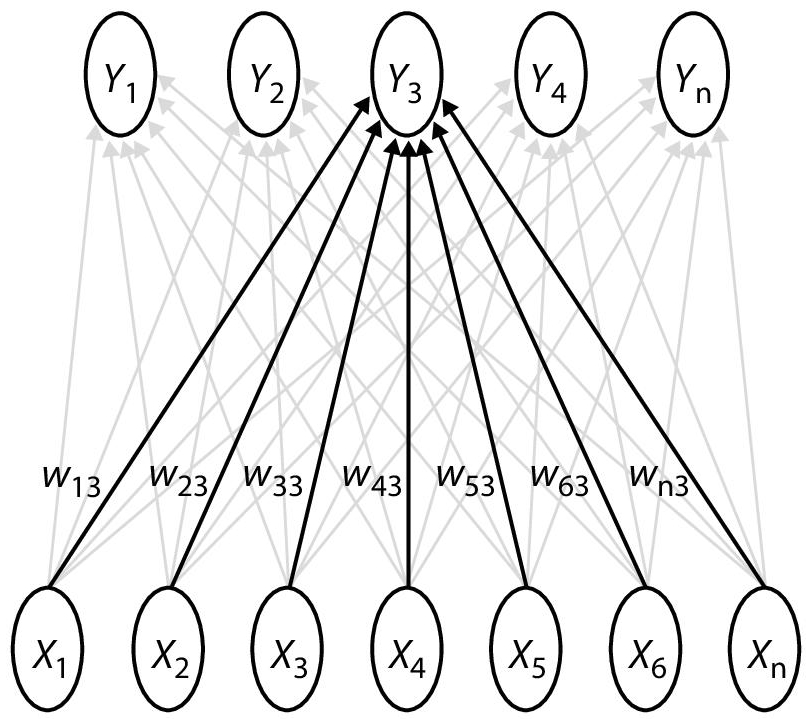
Figure 8.7 Example of self-organizing map (SOM).
8.4 Conclusion
Since wireless sensor networks vary from conventional networks in a variety of ways, protocols and tools that overcome specific problems and limitations are needed. As a result, creative technologies for energy-aware and real-time routing, protection, scheduling, localization, node clustering, data aggregation, fault detection, and data integrity are needed for wireless sensor networks. Machine learning is a collection of strategies for improving a wireless sensor network’s ability to respond to the complex behaviour of its surroundings. However, the concept of area establishes the parameters for how such a relationship can be carried out.
References
- 1. Ayodele, T.O., Introduction to computer learning, in: New Advances in Machine Learning, InTech, 17–26, 2010.
- 2. Duffy, A.H., The “what” and “how” in design learning. IEEE Expert, 12, 3, 71–76, 1997.
- 3. Langley, P. and Simon, H.A., Applications of machine learning and rule induction. Commun. ACM, 38, 11, 54–64, 1995.
- 4. Paradis, L. and Han, Q., A study of fault control in wireless sensor networks. J. Netw. Syst. Manage., 15, 2, 171–190, 2007.
- 5. Krishnamachari, B., Estrin, D., Wicker, S., The effects of data aggregation in wireless sensor networks. 22nd International Conference on Distributed Computing Systems Workshops, pp. 575–578, 2002.
- 6. Al-Karaki, J. and Kamal, A., Routing techniques in wireless sensor networks: A survey. IEEE Wirel. Commun., 11, 6, 6–28, 2004.
- 7. Das, S., Abraham, A., Panigrahi, B.K., Computational intelligence: Foundations, insights, and recent trends, pp. 27–37, John Wiley & Sons, Inc, 2010.
- 8. Conte, R., Gilbert, N., Sichman, J.S., MAS and social simulation: A suitable commitment, in: Multi-Agent Systems and Agent-Based Simulation. MABS 1998. Lecture Notes in Computer Science, vol. 1534. Springer, Berlin, Heidelberg, 1998, https://doi.org/10.1007/10692956_1.
- 9. Nand, P. and Sharma, S.C., Comparison of MANET routing protocols and performance analysis of the DSR protocol, in: Advances in Computing, Communication and Control, vol. 125, 2011.
- 10. Das, S.R., Castaeda, R., Yan, J., Simulation-based performance assessment of routing protocols for mobile ad hoc networks. Mobile Netw. App., l, 5–11, 2000.
- 11. Khetmal, C., Kelkar, S., Bhosale, N., MANET: Black hole node detection in AODV. Int. J. Comput. Eng. Res., 03–09, 2013.
- 12. Abbasi, A.A. and Younis, M., A study on clustering algorithms for wireless sensor networks, 07–12, 2019.
- 13. Yun, S., Lee, J., Chung, W., Kim, E., Kim, S., A soft computing approach to localization in wireless sensor networks. Expert Syst. Appl., 36, 4, 7552–7561, 2009.
- 14. Kannan, S. et al., Secure data transmission in MANETs using AODV. IJCCER, 02–09, 2014.
Note
- Email: [email protected]