
Chapter 5
Binaural Audio Through Loudspeakers
Introduction
Background and Motivation
The ultimate goal of binaural audio with loudspeakers (BAL), also known as transauralization (Cooper & Bauck, 1989), is to reproduce, at each of the listener’s eardrums, the sound pressure signals recorded on only the ipsilateral channel of a stereo signal. If the stereo signal1 was encoded with the head-related transfer function (HRTF) of the listener, and includes the proper ITD (interaural time difference) and ILD (interaural level difference) cues, then delivering the signal on each channel of the stereo recording to the ipsilateral ear, and only to that ear, would ideally guarantee that the listener’s ear-brain system receives the cues it needs to perceive an accurate three-dimensional reproduction of the recorded sound field. Since, with playback from two loudspeakers, each of the cues is also heard by the contralateral ear (crosstalk), accurate 3D audio reproduction through BAL requires an effective cancellation of this unintended crosstalk. Without such crosstalk cancellation (XTC), the ITD and ILD cues will inevitably be corrupted.
In addition to XTC, effective BAL requires an abatement of sound reflections in the listening room, since such reflections directly degrade the integrity of the binaural cues at the listener’s ears (Damaske, 1971; Sæbø, 2001). While this problem can be somewhat alleviated through prescriptions that increase the ratio of direct to reflected sound, accurate sound localization through BAL has been shown to require XTC levels2 above 20 dB (Parodi & Rubak, 2011b), which are difficult to achieve practically even under anechoic conditions (Akeroyd et al., 2007).
Therefore, it would seem that the goal stated in the first paragraph could be more naturally reached with binaural audio through headphones (or earphones), as both crosstalk and room reflections would be non-existent. However, with headphones or earphones, the location of the playback transducers in or very near the ears means that non-idealities (e.g., mismatches between the HRTF of the listener and that used to encode the recording, movement of the perceived sound image with movement of the listener’s head, lack of bone-conducted sound, transducer induced resonances in the ear canal, discomfort, etc.), when above a certain threshold, can lead to difficulties in perceiving a realistic three-dimensional image and to the perception that the sound (or some of its spectral components) is inside, or too close to, the listener’s head (see Chapter 4 and Nicol, 2010, for a more thorough discussion of this issue).
Binaural playback through loudspeakers is largely immune to this head internalization of sound because, even when non-idealities in binaural reproduction are present, the sound originates far enough from the listener to be perceived to come from outside the head. Furthermore, cues such as bone-conducted sound and the involvement of the listener’s own head, torso, and pinnae in sound diffraction and reflection during playback (even if it departs from, or interferes with, the diffraction-induced coloration represented in the HRTF used to encode the binaural recording) could be expected to enhance the perceived realism of sound reproduction relative to that achieved with earphones. These potential advantages have, implicitly or explicitly, motivated the development of XTC-enabled BAL since the earliest work on the subject (Atal, Hill & Schroeder, 1966; Bauer, 1961; Damaske, 1971 and Chapter 2).
Some applications of BAL, such as immersive virtual reality environments or scientific studies of spatial hearing, require binaural cues to be transmitted to a listener with a high degree of fidelity and reliability. Such transparency and robustness often require anechoic (or semi-anechoic) environments (or equivalently, high-directivity loudspeakers that abate the prominence of reflected sound), individualization of the XTC system for the listener and the playback set-up, precise matching of the listener’s HRTF with that used in the recording, and either constraining the position of the listener’s head in the area of equalization (the “sweet spot”) (Akeroyd et al., 2007; Majdak, Masiero & Fels, 2013; Moore, Tew & Nicol, 2010; Parodi & Rubak, 2011b) or adding the complexity of a head-tracking system. However, in many less stringent applications, modest levels of XTC, even of a few dB over a limited range of frequencies, have the potential to significantly enhance the three-dimensional realism of the reproduction of recordings containing binaural cues. This is because, by definition, localization cues in a binaural recording represent differential interaural information that is intended to be transmitted to the ears with no crosstalk. In other words, crosstalk cancellation, at any level, is a reduction of unintended corruption in the loudspeaker playback of recordings containing significant binaural cues.
This reduction of unintended corruption through XTC should also apply to the loudspeaker playback of most stereo recordings,3 especially those made in real acoustic spaces, and even to recordings made using standard stereo microphone techniques without a dummy head, because these techniques all rely on preserving in the recording a good measure of the natural ITD and ILD cues needed for enhancing the accuracy of spatial localization and the realism of hall reverberation during playback (Hugonnet & Walder, 1997). We should therefore expect that effecting even a relatively low level of XTC in the playback of such standard stereo recordings, even those lacking HRTF encoding, should enhance image localization compared to playback with full crosstalk, as well as the perception of width and depth of the sound field, since these binaural features are always, to some degree, corrupted by crosstalk.4
Before addressing the most fundamental challenge in XTC filter design, we list some of the practical challenges encountered when implementing an effective XTC-enabled BAL playback system and refer to the literature that discusses effective solutions to these practical problems. As alluded to above, such XTC systems are typically sensitive to room reflections (Akeroyd et al., 2007; Damaske, 1971; Sæbø, 2001; Ward, 2001), require the use of specialized playback set-ups (Kirkeby, Nelson & Hamada, 1998a, b; Takeuchi & Nelson, 2002, 2007), and necessarily create a single restricted sweet spot in which the XTC is effective (Takeuchi, Nelson & Hamada, 2001; Ward & Elko, 1999; Xie, 2013, and references therein). Much research effort has been expended on how to relieve the latter constraint and has resulted in potential solutions, of varying degrees of practicality, which include widening the sweet spot through the use of multiple loudspeakers (Bai, Tung & Lee, 2005; Takeuchi & Nelson, 2002; Yang, Gan & Tan, 2003) and/or elevated loudspeakers (Parodi & Rubak, 2010), providing XTC at multiple listening locations through the use of multiple loudspeaker pairs (Bauck & Cooper, 1996; Kim, Deille & Nelson, 2006), and dynamically moving the sweet spot to follow the location of the listener’s head by tracking it with optical sensors (Gardner, 1998; Lentz, 2006; Mannerheim, 2008).
The most fundamental challenge in XTC filter design is dealing with the tonal distortion (spectral coloration)5 that XTC filters inherently impose on the sound emitted by the loudspeakers. As we will show in the following sections, the level of tonal distortion depends on the location of the sound source in the sound field, and therefore cannot be corrected through equalization, especially for audio signals containing more than a single sound source. The basic problem of XTC, the fundamental nature of the associated tonal distortion, its main features, its dependencies, and, ultimately, the formulation of a method for the practical design of optimal XTC filters that abate such tonal distortion with minimal degradation of XTC performance are the main subjects of this chapter.
The Problem of XTC-Induced Tonal Distortion
Nature of the Problem
One main difficulty in implementing XTC is to reduce the artifice of crosstalk without adding an artifice of another kind: tonal distortion. Sound waves traveling from two distinct sources to the ears set up an interference pattern in the intervening air space. Depending on the frequency, the distances between an ear and the loudspeakers, the distance between the loudspeakers, and the phase relationship between the left and right components of the recorded stereo signal, the wave interference at that ear of the listener might be constructive, destructive, or complementary (90° out of phase). At the frequencies for which the interference between in-phase recorded signals is destructive at the ears (or, alternatively, the frequencies for which the interference between out-of-phase signals is constructive), XTC control (i.e., signal processing that would cause the waves from the loudspeakers to the contralateral ears to be nulled) would require boosting the amplitude of the emitted waves (Takeuchi & Nelson, 2002).6 As shown in the section “Benchmark: Perfect Crosstalk Cancellation,” in the case of a perfect XTC filter (defined as one that theoretically yields, in a free-field or anechoic environment, an infinite XTC level over the entire audio band) for typical listening configurations, these level boosts can easily be in excess of 30 dB, and therefore amount to severe tonal distortion.
Of course, such a “perfect” XTC filter would impose these necessary level boosts only at the loudspeakers in such a way that, at the listener’s ears, not only is the crosstalk cancelled, but the frequency spectrum is also reconstructed perfectly, i.e., with no tonal distortion.
As recognized by Takeuchi and Nelson (2002) and P. A. Nelson and Rose (2005), and as further discussed in the section “Benchmark: Perfect Crosstalk Cancellation,” the frequencies at which the level boosts are required correspond to the frequencies at which the system inversion (the mathematical inversion of the system’s transfer matrix, which leads to the XTC filter) is ill conditioned. As a result, XTC control becomes highly sensitive to errors at these frequencies, so that even a small error in the alignment of the listener’s head in the real world would lead to a significant loss of XTC control at and near these frequencies. Therefore, not only would there be undesired crosstalk at the listener’s ears at these frequencies, but also and consequently, the level boosts which must necessarily be imposed at these frequencies would be fully audible, even in the sweet spot, as coloration (tonal distortion).
Takeuchi and Nelson (2002) show that, even in an ideal world where the loudspeakers–listener alignment is perfect, this tonal distortion imposed at the loudspeakers would present three problems: 1) it would be heard by a listener outside the sweet spot, 2) it would cause a relative increase (compared to unprocessed sound playback) in the physical strain on the playback transducers, and 3) it would correspond to a loss in dynamic range. Since even professional audio equipment is seldom designed to have more than a few dB headroom above the levels required to reproduce the full dynamic range of realistic sound pressures (Katz, 2002), in order to avoid clipping in the case of the “perfect” XTC filter defined above, the dynamic range of the program would need to be decreased by more than 30 dB (minus the headroom). This is particularly problematic, for instance, in the case of wide-dynamic-range audio recorded in 16 or 24 bits (see Chapter 2 and references to these early efforts in the Bibliography of this chapter).
Previous Work and Goals of This Chapter
The history of crosstalk cancellation extends back to the seminal work of Bauer, Atal, Hill and Schroeder in the early 1960s (see references to these early efforts in the Bibliography of this chapter) and has since progressed at a faster rate with the advent of digital audio for which XTC can be readily implemented through digital filtering. We shall not attempt to review this history here, nor the various methods of implementing XTC (which range from older techniques applied in the analog domain (Atal et al., 1966), to time-domain signal manipulation algorithms, such as the RACE algorithm (Glasgal, 2007), and FFT-based digital convolution with finite impulse response (FIR) filters (SreenivasaRao, Mahalakshmi & VenkataRao, 2012), and instead focus our discussion on the problem of tonal distortion in XTC filters.
Takeuchi and Nelson (2002) have developed a method that not only yields excellent measured XTC performance (see also Akeroyd et al., 2007; Takeuchi & Nelson, 2007), but also effectively solves the problem of tonal distortion. However, their method, called the “Optimal Source Distribution” (OSD), which is discussed in the section “Benchmark: Perfect Crosstalk Cancellation,” requires the use of a minimum of four (but typically six) transducers positioned at various angles around the listener.
The problem of XTC-induced tonal distortion for playback with only two loudspeakers remains compelling due to the simplicity of the two-loudspeaker set-up and its compatibility with existing audio equipment. In this chapter, we study this problem in the context of XTC optimization, which we define as the maximization of XTC performance for a desired tolerable level of tonal distortion or, equivalently, the minimization of tonal distortion for a desired XTC performance.
The ultimate goal of the discussion in this chapter is to describe the design of “optimal XTC filters” (called BACCH filters) that do not suffer from the following drawbacks inherent to regular XTC filters:
- D1: Severe tonal distortion to the sound heard by the listener, even if that listener is sitting in the intended sweet spot.
- D2: Useful XTC levels are reached only at limited frequency ranges of the audio band.
- D3: Severe dynamic range loss when the sound is processed through the XTC filter or processor (while avoiding distortion and/or clipping).
In particular, we use a free-field two-point-source model and address, analytically, the fundamental aspects of tonal distortion control through both constant-parameter (frequency- independent) and frequency-dependent regularization methods. The use of regularization in the design of XTC filters was proposed by Kirkeby and colleagues (1998) to make the inversion of the system transfer matrix better behaved, and has since seen widespread adoption in the field. Specifically, constant-parameter regularization has been employed to control ill-conditioning in the design of HRTF-based XTC filters (e.g., Akeroyd et al., 2007; Kirkeby et al., 1998; Majdak et al., 2013), and frequency-dependent methods have been employed to tame high- and low-frequency amplification due to measured-HRTF inversion (e.g., Kirkeby & Nelson, 1999; Moore et al., 2010) and to control the temporal extent of the XTC filters (e.g., Parodi & Rubak, 2010, 2011a). Regarding the issues of tonal distortion and dynamic range loss, Papadopoulos and Nelson (2010) used constant-parameter regularization to limit the dynamic range loss inflicted by XTC, and Bai et al. (2005) and Bai & Lee (2006a) employed frequency-dependent regularization to impose gain limits on the XTC filters.
In the section “Constant-Parameter Regularization,” we show that while the technique of constant-parameter (non-frequency-dependent) regularization may alleviate some of drawback D3, it inherently introduces spectral artifice of its own (specifically, while reducing the amplitude of the spectral peaks in the inverted transfer matrix, constant-parameter regularization results in undesirable narrow-band artifacts at higher frequencies and a roll-off at lower frequencies at the loudspeakers) and does little to alleviate the other two drawbacks (D1 and D2).
A discussion of the fundamental aspects of frequency-dependent regularization in the section “Frequency-Dependent Regularization” will lead us to our ultimate goal: a method for designing “optimal XTC filters” called “BACCH filters.” The method relies on calculating the frequency-dependent regularization parameter (FDRP) that results in a flat amplitude versus frequency response at the loudspeakers (as opposed to a flat amplitude versus frequency response at the ears of the listener, as in previous design methods), thus forcing XTC to be effected into the phase domain only and relieving the XTC filter from the drawbacks of audible tonal distortion and dynamic range loss. When the method is used with any effective optimization scheme, it results in XTC filters that yield optimal XTC levels over any desired portion of the audio band, impose no tonal distortion on the processed sound beyond the tonal distortion inherent in the playback hardware and/or loudspeakers, and causes no dynamic range loss. XTC filters designed with this method and used in the system are not only optimal but, due to their being free from drawbacks D1, D2, and D3, allow for a most natural and spectrally transparent 3D audio reproduction of binaural or stereo audio through loudspeakers.
The Fundamental XTC Problem
In this section, we start with the mathematical formulation of the model and the governing transformation matrices. We then define a set of metrics that are useful for evaluating and comparing the tonal distortion and performance of XTC filters, and conclude with the definition and discussion of a benchmark for such comparisons: the perfect XTC filter.
Formulation and Transformation Matrices
In order to render the analysis tractable enough so that fundamental insight is more easily obtained, we make the idealizing assumptions that sound propagation occurs in a free field (with no diffraction or reflection from the head and pinnae of the listener or any other physical objects), and that the loudspeakers radiate like point sources.
In the frequency domain, the air pressure at a free-field point located a distance r from a point source (monopole) radiating a sound wave of frequency ω is given by Morse and Ingard (1986)
where ρ0 is the air density, k = 2π/λ = ω/cs the wavenumber, λ the wavelength, cs the speed of sound (340.3 m/s), and q the source strength (in units of volume per unit time). It is convenient to define
which is the time derivative of ρ0q/4π, the mass flow rate of air from the center of the source.
Therefore, at the left ear of a listener in the symmetric two-source geometry shown in Figure 5.1, the air pressure due to the two sources, under the above-stated assumptions, add up as
|
PL(iω)=e−ikl1l1VL(iω)+e−ikl2l2VR(iω) |
(5.1) |
Similarly, at the right ear, we have
|
PR(iω)=e−ikl2l2VL(iω)+e−ikl1l1VR(iω) |
(5.2) |
Here, l1 and l2 are the path lengths between either source and the ipsilateral and contralateral ears, respectively, as shown in that figure.
In order to maintain a connection with the relevant literature, we adopt the same nomenclature used by Kirkeby et al. (1998a, b), Takeuchi and Nelson (2002), and P. A. Nelson and Rose (2005). Namely, unless otherwise stated, we use uppercase letters for frequency variables, lowercase for time-domain variables, uppercase bold for matrices, and lowercase bold for vectors, and define
| ∆l ≡ l2 - l1 and g ≡ l1/l2 | (5.3) |
as the path length difference and path length ratio, respectively. An inspection of the geometry illustrated in Figure 5.1 shows that 0 < g < 1, and that the path lengths can be expressed as
|
l1=√l2+(Δr2)2−Δrl sin(θ), |
(5.4) |
|
l2=√l2+(Δr2)2−Δrl sin(θ), |
(5.5) |

where ∆r is the effective distance between the entrances of the ear canals, and l is the distance between either source and the interaural mid-point. As defined in Figure 5.1, 2θ = Θ is the loudspeaker span. Note that for l ≫ ∆r sin (θ), as in most loudspeaker-based listening set-ups, we have g ≃ 1. Another important parameter is the time delay,
|
τc=Δlcs, |
(5.6) |
defined as the time it takes a sound wave to traverse the path length difference ∆l.
Using the above definitions, Equations (5.1) and (5.2) can be re-written in matrix form as
|
[PL(iω)PR(iω)]=α[1ge−iωτcge−iωτc1][VL(iω)VR(iω)] |
(5.7) |
where
|
α=e−iωl1/csl1 |
(5.8) |
In the time domain, α is simply a transmission delay (divided by the constant l1) that does not affect the shape of the signal. Its role in ensuring causality is discussed in the section “Metrics.” The source vector v = [VL(iω), VR(iω)]T is obtained from the vector of “recorded” signals d = [DL(iω), DR(iω)]T, through the transformation
| v = Hd, | (5.9) |
where
|
H=[HLL(iω)HLR(iω)HRL(iω)HRR(iω)] |
(5.10) |
is the sought 2 × 2 filter matrix. Therefore, from Equation (5.7), we have
| p = αCHd | (5.11) |
where p = [PL(iω), PR(iω)]T is the vector of pressures at the ears, and C is the system’s transfer matrix
|
C≡[1ge−iωτcge−iωτc1], |
(5.12) |
which, like all matrices we deal with here, is symmetric due to the symmetry of the geometry.
In summary, the transformation from the signals d, through the filter matrix H, to the source variables v, then through wave propagation from the sources to the pressures p at the ears of the listener, can be written simply as
| p = αRd | (5.13) |
where we have introduced the performance matrix, R, defined as
|
R=[RLL(iω)RLR(iω)RRL(iω)RRR(iω)]≡CH. |
(5.14) |
Metrics
We now wish to define a set of metrics by which to judge the tonal distortion and performance of XTC filters. In this context, we note that the diagonal elements of R represent the ipsilateral transmission of the signal to the ears, and the off-diagonal elements represent the undesired contralateral transmission, i.e., the crosstalk.
The responses of the system to a signal fed to only one (either left or right) of the two inputs, as heard at the ears, are called the “side images” of the system (i.e., either αR·[1,0]T or αR·[0,1]T). We define our first coloration metric as the amplitude spectrum (to a factor α) of the side image at the ipsilateral ear, given by
ESi (ω) ≡ |RLL(iω)| = |RRR(iω)|,
where the subscripts “si” and “||” stand for “side image” and “ipsilateral ear (with respect to the input signal),” respectively. Similarly, at the contralateral ear to the input signal (subscript “X”), we have the following side-image amplitude spectrum:
The response of the system to a signal split equally between left and right inputs, as heard at either ear, is called the “center image” of the system (i.e., αR · [1/2,1/2]T). We define another coloration metric as the amplitude spectrum of the center image, given by
where the subscript “ci” stands for “center image.”
Also of importance to our discussions are the frequency responses that would be measured at the sources (loudspeakers). These are denoted by S, and can be obtained from the elements of the filter matrix H. They are given using the same subscript convention used above (with “‖” and “X” referring to the loudspeakers that are ipsilateral and contralateral to the input signal, respectively) by
An intuitive interpretation of the significance of the above metrics is that a signal panned from a single input to both inputs to the system will result in frequency responses going from Esi to Eci at the ears, and Ssi to Sci at the loudspeakers.
Two other tonal distortion metrics are the frequency responses of the system to in-phase and out-of-phase inputs to the system. These two responses are obtained simply from the product of the filter matrix H with the vectors [1,1]T and [1,−1]T (or [−1,1]T), respectively, and are given by:
where the subscripts “i” and “o” denote the in-phase and out-of-phase responses, respectively. Note that, as defined, Si is double (i.e., 6 dB above) Sci , as the latter describes a signal of amplitude 1 panned to center (i.e., split equally between L and R inputs), while the former describes two signals of amplitude 1 fed in-phase to the two inputs of the system.
Since a real signal can consist of various components having different phase relationships, it is more useful to combine Si(ω) and So(ω) into a single metric, Ŝ(ω), which is the envelope spectrum that describes the maximum amplitude that could be expected at the loudspeakers, and is given by
Ŝ(ω) = max[Si(ω), So (ω)].
It is relevant to note that Ŝ(ω) is equivalent to ‖ H ‖, the 2-norm of H, and that Si and So are the two singular values, which can be obtained through singular value decomposition of the matrix, as was done by Takeuchi and Nelson (2002).
Finally, an important metric that allows us to evaluate and compare the XTC performance of various filters is χ(ω), the crosstalk cancellation spectrum:
The above definitions give us a total of eight metrics, (Esi‖, EsiX, Eci, Ssi‖, SsiX, Sci, Ŝ, and χ), all real functions of frequency, by which to evaluate and compare the tonal distortion and XTC performance of XTC filters.
Benchmark: Perfect Crosstalk Cancellation
A perfect crosstalk cancellation (P-XTC) filter is defined as one that, theoretically, yields infinite crosstalk cancellation at the ears of the listener, for all frequencies.
Crosstalk cancellation, as defined in the section “Background and Motivation,” requires that the pressure at each of the two ears be that which would have resulted from the ipsilateral signal alone, namely, in the frequency domain, PL = αDL and PR = αDR, where all quantities are complex functions of frequency. Therefore, in order to achieve perfect cancellation of the crosstalk, Equation (5.13) requires that R = I, where I is the identity matrix, and thus, as per the definition of R in Equation (5.14), the P-XTC filter is simply the inverse of the system transfer matrix expressed in Equation (5.12), and can be expressed exactly:
|
H[P]=C-1=11−g2e−2iωτc[1−ge−iωτc−ge−iωτc1], |
(5.15) |
where the superscript “[P]” denotes perfect XTC. For this filter, the eight metrics we defined above become:
|
E[P]sin= 1;E[P]siX= 0;E[P]ci=12S [P]sin(ω) =|11−g2e−2iωτc| =1√g4−2g2 cos(2ωτc)+1;S [P]siX(ω) =|−ge−iωτc1−g2e−2iωτc| =g√g4−2g2 cos(2ωτc)+1;S [P]ci(ω) =12|1−gg+eiωτc| =12√g2+2g cos(ωτc)+1;∧S [P](ω) =max(|1−gg+eiωτc|,|1+geiωτc−g|) = max(1√g2+2g cos(ωτc)+11√g2+2g cos(ωτc)+1); |
(5.16) |
| χ[P] (ω) = ∞ | (5.17) |
Therefore, the perfect (χ = ∞) XTC filter gives flat frequency responses at the ears (E[P](ω) = constant), but not at the sources. To appreciate the extent of tonal distortion at the loudspeakers, we plot the S[P](ω) frequency responses expressed above in Figure 5.2 for a typical value of g = 0.985. Throughout this chapter, for the sake of illustration, we complement the non-dimensional plots with dimensional calculations, which are represented by the same curves read in terms of the frequency f = ω/2π on the top axis, for a typical listening geometry characterized by g = 0.985 and τc = 68 µs (i.e., 3 samples at the “Red Book” CD sampling rate of 44.1 kHz), which would be the case, for instance, in a set-up with ∆r = 15 cm, l = 1.6 m, and Θ = 18°.
The peaks in these spectra occur at frequencies for which the system must boost the amplitude of the signal at the loudspeakers in order to effect XTC at the ears while compensating for the destructive interference at that location. Similarly, minima in the spectra occur when the amplitude must be attenuated.

Using the first and second derivatives (with respect to ωτc) of the above expressions for the various S[P](ω) spectra, we find the following amplitudes and frequencies for the associated peaks and minima, denoted by “↑” and “↓” superscripts, respectively:
|
S [P]↑sin=11−g2at ωτc=nπ,S [P]↓sin =11−g2at ωτc=(2n+1)π2,S [P]↑six =11−g2at ωτc=nπ,S [P]↓six =11−g2at ωτc=(2n+1)π2,S [P]↑ci =12−2gat ωτc=(2n+1)π,S [P]↓ci =12−2gat ωτc=2nπ,∧S [P]↑=11−g at ωτc=nπ, |
(5.18) |
|
∧S [P]↓=1√1+g2 at ωτc=(2n+1)π2, |
(5.19) |
with n = 0,1,2,3,4,… .
For a typical listening set-up, g ≃ 1, say, our reference g = 0.985 case shown in Figure 5.2, the envelope peaks (i.e., Ŝ [P]↑) correspond to a boost of
(and the peaks in the other spectra, Ssi[P]↑≃↑≃ Sci[P]↑ correspond to boosts of about 30.5 dB). While these boosts have equal frequency widths across the spectrum, when the spectrum is plotted logarithmically (as is appropriate for human sound perception), the low-frequency boost is most prominent in its perceived frequency extent. This “bass boost” has long been recognized as an intrinsic problem in XTC (Kirkeby et al., 1998b; Takeuchi & Nelson, 2002). While the high-frequency peaks could, in principle, be pushed out of the audio range by decreasing τc (which, as can be seen from Equations (5.4)–(5.6), is achieved by increasing l and/or decreasing the loudspeaker span Θ, as is done in the so-called Stereo Dipole configuration described by Kirkeby, Nelson and Hamada (1998a, b), where Θ = 10°), the low-frequency boost of the P-XTC filter would remain problematic.
As mentioned in the section “The Problem of XTC-Induced Tonal Distortion,” the severe tonal distortion associated with these high-amplitude peaks presents three practical problems: 1) it would be heard by a listener outside the sweet spot, 2) it would cause a relative increase (compared to unprocessed sound playback) in the physical strain on the playback transducers, and 3) it would correspond to a loss in the dynamic range.
These penalties might be a justifiable price to pay if we are guaranteed the infinitely good XTC performance (χ = ∞) and the perfectly flat frequency response (E[P](ω) = constant) that the perfect XTC filter promises at the ears of a listener in the sweet spot. However, in practice, these theoretically promised benefits are unachievable due to the solution’s sensitivity to unavoidable errors. This problem can best be appreciated by evaluating the condition number of the transfer matrix C.
In matrix inversion problems, the sensitivity of the solution to errors in the system is given by the condition number of the matrix. (For a discussion of the condition number in the context of XTC system errors, see P. A. Nelson and Rose, 2005.) The condition number κ(C) of the matrix C is given by
κ(C) = ||C|| ∙ ||C-1|| = ||C|| ∙ ||H[P]||.
(It is also, equivalently, the ratio of largest to smallest singular values of the matrix.) Therefore, we have
Using the first and second derivatives of this function, as we did for the previous spectra, we find the following maxima and minima:
|
κ↑(C)=1+g1−g at ωτc=nπ,κ↓(C)=1 at ωτc=(2n+1)π2 |
(5.20) |
with n = 0,1,2,3,4, . . .,
as was also reported by Ward and Elko (1999) and P. A. Nelson and Rose (2005) in terms of wavelengths, and by Takeuchi and Nelson (2002) in terms of the wave number. First, we note that the maxima and minima in the condition number occur at the same frequencies as those of the amplitude envelope spectrum at the loudspeakers, Ŝ [P]. Second, we note that the minima have a condition number of unity (the lowest possible value), which implies that the filter resulting from the inversion of C is most robust (i.e., least sensitive to errors in the transfer matrix) at the non-dimensional frequencies ωτc = π/2, 3π/2, 5π/2, . . .. Conversely, the condition number can reach very high values (e.g., κ↑(C) = 132.3 for our typical case of g = 0.985) at the non-dimensional frequencies ωτc = 0, π, 2π, 3π, . . .. As g → 1, the matrix inversion resulting in the P-XTC filter becomes ill conditioned, or, in other words, infinitely sensitive to errors. The slightest misalignment, for instance, of the listener’s head, would thus result in a severe loss in XTC control at the ears (at and near these frequencies) which, in turn, causes the severe tonal distortion in Ŝ [P](ω) to be transmitted to the ears.
We are now in a position to appreciate the prescription proposed and implemented by Takeuchi and Nelson (2002, 2007), which effectively solves both the robustness and tonal distortion problem of the P-XTC filter by ensuring that the system operates always under conditions where κ(C) is small. This can be done by allowing the loudspeaker span to be a function of the frequency. More specifically, after noting that typically l ≫ ∆r, so that the approximation ∆l ≃ ∆r sin(θ) holds, and therefore ωτc = ω∆l/cs = 2πf∆l/cs can be approximated by
| ωτc⋍2πfΔsin (θ)cs for l⋍Δr, | (5.21) |
we can re-write the robustness condition (stated in Equation (5.20)) as
with n = 0,1,2,3,4, . . .
Since both cs and ∆r are constant, the required loudspeaker span is solely a function of the frequency f. In practice, this prescription, called Optimal Source Distribution (OSD), can be implemented by using a crossover network to distribute adjacent bands of the audio spectrum to pairs of transducers, whose spans are calculated from the above equation so that in each band the condition number does not exceed unity by much, thus insuring robustness and low coloration over the entire audio spectrum. It is clear, however, that this solution is not applicable to the case of a single pair of loudspeakers, which is the focus of our analysis.
We refer the reader interested in the OSD method and XTC errors to Takeuchi and Nelson (2002, 2007) and P. A. Nelson and Rose (2005), and sum up the discussion in this section by stating that, for the case of only two loudspeakers, the perfect XTC filter carries in practice the penalties of over-amplification (and the associated loss of dynamic range) at frequencies where system inversion is ill conditioned, transducer fatigue, and a severe tonal distortion that is heard by listeners inside and outside the sweet spot.
Constant-Parameter Regularization
Regularization methods allow controlling the norm of the approximate solution of an ill-conditioned linear system at the price of some loss in the accuracy of the solution. The control of the norm through regularization can be done subject to an optimization prescription, such as the minimization of a cost function. Hansen (1998) provides a detailed discussion of regularization methods in a general mathematical context, and others (e.g., Bai et al., 2005; Kirkeby & Nelson, 1999; Majdak et al., 2013; Parodi & Rubak, 2010) have demonstrated the use of regularization to control numerical HRTF inversion. We discuss regularization analytically in the context of XTC filter optimization, which we define as the maximization of XTC performance for a desired tolerable level of tonal distortion or, equivalently, the minimization of tonal distortion for a desired minimum XTC performance.
In essence, a nearby solution to the matrix inversion problem is sought:
| H[β] = [CHC + βI]-1CH, | (5.22) |
where the superscript “H” denotes the conjugate transpose, and β is the regularization parameter which essentially causes a departure from H[P], the exact inverse of C. In this section we take β to be a constant. The pseudoinverse matrix H[β] is the regularized filter, and the superscript “[β]” is used to denote constant-parameter regularization. The regularization stated in Equation (5.22) can be shown to correspond to a minimization of a cost function, J(iω), where
| J(iω) = eH(iω)e(iω) + βvH(iω)v(iω) | (5.23) |
and the vector e represents a performance metric that is a measure of the departure from the signal reproduced by the perfect filter (Kirkeby et al., 1998; P. A. Nelson & Elliott, 1993). Physically, then, the first term in the sum constituting the cost function represents a measure of the performance error, and the second term represents an “effort penalty,” which is a measure of the power exerted by the loudspeakers. For β > 0, Equation (5.22) leads to an optimum, which corresponds to the least-squares minimization of the cost function J(iω).
Therefore, an increase of the regularization parameter β leads to a minimization of the effort penalty at the expense of a larger performance error, and thus to an abatement of the peaks in the norm of H, i.e., the coloration peaks in the S(ω) spectra, at the price of a decrease in XTC performance at and near the frequencies where the system is ill conditioned.
Frequency Response
Using the explicit form for C given by Equation (5.12), in the last equation above, we find:
| H[β]=[H[β]LL(iω)H[β]LR(iω)H[β]RL(iω)H[β]RR(iω)], | (5.24) |
where
| H[β]RR(iω)=H[β]RR(iω) = g2e4iωτc−(β+1)e2iωτcg2e4iωτc+g2−e4iωτc[(g2+β )2+2β+1], | (5.25) |
| H[β]LR(iω)=H[β]RL(iω) = g2eiωτc−g(g2+β )e3iωτcg2e4iωτc+g2−e2iωτc[(g2+β )2+2β+1], | (5.26) |
The eight metric spectra we defined in the section “Metrics” become:
| E [β]si⋍(ω)=g4+βg2−2g2 cos(2ωτc)+β+1−2g2 cos(2ωτc)+(g2+β)2+2β+1;E [β]siX(ω)=2gβ⋅|cos(ωτc)| −2g2 cos(2ωτc)+(g2+β)2+2β+1;E [β]ci(ω)=12−β 2[g2+2g cos(2ωτc)+ β+1];S [β]si⋍(ω)=√g4+2(β+1)g2 cos(2ωτc)+(β+1)2−2g2 cos(2ωτc)+(g2+β)2+2β+1;S [β]siX(ω)=g√(g2+β)2−2(g2+β) cos(2ωτc)+1−2g2 cos(2ωτc)+(g2+β)2+2β+1;S [β]ci(ω)=√g2+2g cos(ωτc)+12 [g2+2g cos(2ωτc)+β+1];∧S [β](ω)=max(√g2+2g cos(ωτc)+1g2+2g cos(2ωτc)+β+1√g2−2g cos(ωτc)+1g2−2g cos(2ωτc)+β+1); | (5.27) |
| χ[β](ω)=g4+βg2−2g2cos(2ωτc)+β+1 2gβ⋅|cos(2ωτc)|; | (5.28) |
Of course, as β → 0, H[β] → H[P], and it can be verified that the spectra of the perfect XTC filter are recovered from the expressions above.
The envelope spectrum, Ŝ [β](ω), is plotted in Figure 5.3 for three values of β. Two features can be noted in that plot: 1) increasing the regularization parameter attenuates the peaks in the spectrum without affecting the minima, and 2) with increasing β, the spectral maxima split into doublet peaks (two closely spaced peaks).
To get a measure of peak attenuation and the conditions for the formation of doublet peaks, we take the first and second derivatives of Ŝ [β](ω) with respect to ωτc and find the conditions for which the first derivative is nil and the second is negative. These conditions are summarized as follows: If β is below a threshold β* defined as
| β < β* ≡ (g - 1)2, | (5.29) |
the peaks are singlets and occur at the same non-dimensional frequencies as for the envelope spectrum peaks of the P-XTC filter (Ŝ [P]↑), and have the following amplitude:
with n = 0,1,2,3,4, . . .

If the condition
| β* ≤ β 1 | (5.30) |
is satisfied, the maxima are doublet peaks located at the following non-dimensional frequencies:
| ωτc=nπ±cos−1(g2−β+12g) | (5.31) |
with n = 0,1,2,3,4, . . .,
and have an amplitude
| ∧S [β]↑↑ =12√β, | (5.32) |
which does not depend on g. (The superscripts “↑” and “↑↑” denote singlet and doublet peaks, respectively.) The attenuation of peaks in the Ŝ [β] spectrum due to regularization can be obtained by dividing the amplitude of the peaks in the P-XTC (i.e., β = 0) spectrum by that of peaks in the regularized spectrum. For the case of singlet peaks, the attenuation is
and for doublet peaks, it is given by
For the typical case of g = 0.985 illustrated in Figure 5.3, we have β* = 2.25 × 10⁻⁴, and for β = 0.005 and 0.05, we get doublet peaks that are attenuated (with respect to the peaks in the P-XTC spectrum) by 19.5 and 29.5 dB, respectively, as marked on that plot.
Therefore, increasing the regularization parameter above this (typically low) threshold causes the maxima in the envelope spectrum to split into doublet peaks shifted by a frequency ∆(ωτc) = cos−1[(g2−β+1)/2g] to either side of the peaks in the response of the perfect XTC filter. (For our illustrative case of g = 0.985, we have β* = 2.25 × 10⁻⁴ and ∆(ωτc) ≃ 0.225 for β = 0.05.) Due to the logarithmic nature of frequency perception for humans, these doublet peaks are perceived as narrow-band artifacts at high frequencies (i.e., for n = 1,2,3, . . .), but the first doublet peak centered at n = 0 is perceived as a wide-band low-frequency roll-off of typically many dB, as can be clearly seen in Figure 5.3. Therefore, constant-parameter regularization transforms the bass boost of the perfect XTC filter into a bass roll-off.
Since regularization is essentially a deliberate introduction of error into system inversion, we should expect both the XTC spectrum and the frequency responses at the ears to suffer (i.e., depart from their ideal P-XTC filter levels of ∞ and 0 dB, respectively) with increasing β. The effects of constant-parameter regularization on responses at the ears are illustrated in Figure 5.4.
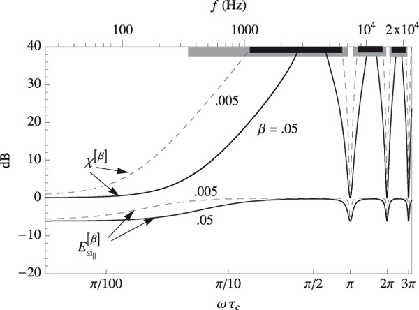
The black curves in that plot represent the crosstalk cancellation spectra and show that XTC control is lost within frequency bands centered around the frequencies where the system is ill conditioned (ωτc = nπ with n = 0,1,2,3,4, . . .) and whose frequency extent widens with increasing regularization. For example, increasing β to 0.05 limits XTC of 20 dB or higher to the frequency ranges marked by black horizontal bars on the top axis of Figure 5.4, with the first range extending only from 1.1 to 6.3 kHz and the second and third ranges located above 8.4 kHz. In many practical applications, such high (20 dB) XTC levels may not be needed or achievable (e.g., because of room reflections and/or HRTF mismatch) and the higher values of β needed to tame the tonal distortion peaks below a required level at the loudspeakers may be tolerated.
The E [β]sin(ω) responses at the ears, shown as the bottom curves in Figure 5.4, depart only by a few dB from the corresponding P-XTC (i.e., β = 0) filter response (which is a flat curve at 0 dB). More precisely and generally, the maxima and minima of the E [β]sin(ω) spectrum are given by:
with n = 0,1,2,3,4, . . .
For the typical (g = 0.985) example shown in the figure, we have, for β = 0.05, and E [β]↑sin=−0.2dB E [β]↑sin=−6.1dB, showing that even relatively aggressive regularization results in a tonal distortion at the ears that is quite modest compared to the tonal distortion the perfect XTC filter imposes at the loudspeakers.
In sum, we conclude that, while constant-parameter regularization is effective at reducing the amplitude of peaks (including the “bass boost”) in the envelope spectrum at the loudspeakers, it typically results in undesirable narrow-band artifacts at higher frequencies and a roll-off of the lower frequencies at the loudspeakers. This non-optimal behavior can be avoided if the regularization parameter is allowed to be a function of the frequency, as we shall see in the section “Frequency-Dependent Regularization.”
Before we do so, it is insightful to consider the effects of constant-parameter regularization on the time-domain response of XTC filters.
Impulse Response
We start by making the substitution z = e2iωτc in Equations (5.25) and (5.26) to get
| H[β]LL(z)=H[β]RR(z) =z2g2−z(β+1)z2g2+g2−z[(g2+β )2+2β+1] | (5.33) |
| H[β]LR(z)=H[β]RL(z) =z2[gz−1/2−g(g2+β)z1/2z2g2+g2−z2[(g2+β)2+2β+1] | (5.34) |
The two expressions above have the same quadratic denominator, which can be factored as
z2g2 + g2 - z[(g2 + β)2 + 2β + 1] = g2(z - a1)(z - a2),
where
| a1=a−√a2−4g42g2, a2=a−√a2−4g42g2, | (5.35) |
and
| a = (g2 + β)2 + 2β+1 | (5.36) |
We can then re-write Equations (5.33) and (5.34) as
| H[β]LL(z)=H[β]RR(z)=[z−( β+1)g2]×(11−a1z−1)(1z−a2), | (5.37) |
| H[β]LR(z)=H[β]RL(z)=[z−1/2−(g2+β )z1/2g2]×(11−a1z−1)(1z−a2). | (5.38) |
Since 0 < g < 1, and β ≥ 0, we see from Equations (5.35) and (5.36) that 0 ≤ a1< 1 and a2> 1, and therefore | a1z−1| < 1 and a2> |z|. This allows us to express the terms 1/(1 − a1z−1) and 1/(z − a2) in the last two equations as two convergent power series (whose convergence insures that we have a stable filter), and thus write the last two equations as
| H[β]LL(z)=H[β]RR(z)=[z−(β+1)g2]×(∑∞m=0am1z−m)(∑∞m=0−a−m−12zm), | (5.39) |
| H[β]LR(z)=H[β]RL(z)=[z−1/2−(g2+β )z1/2g2]×(∑∞m=0am1z−m)(∑∞m=0−a−m−12zm). | (5.40) |
The filter is now in a form that can be readily transformed into a time-domain filter, h[β], represented by
| h[β]=[h[β]LL(t)h[β]LR(t)h[β]RL(t)h[β]RR(t)] | (5.41) |
We do so by substituting back e2iωτc for z in Equations (5.39) and (5.40), and taking the inverse Fourier transform (IFT) to get
| h[β]LL(t)=12π∫∞−∞H[β]LL(iω)eiωtdω =h[β]RR(t)=12π∫∞−∞H[β]RR(iω)eiωtdω [δ(1+2τc)−β+1g2δ(t)]*ψ(t), | (5.42) |
| h[β]LR(t)=12π∫∞−∞H[β]LR(iω)eiωtdω =h[β]LR(t)=12π∫∞−∞H[β]RL(iω)eiωtdω =[δ(t−τc)g−g2+βg2δ(t+τc)]*ψ(t), | (5.43) |
where the asterisk (*) denotes the convolution operation, and ψ(t) is the IFT of the product of the two series appearing in Equations (5.39) and (5.40), and is given by the following convolution of two trains of Dirac delta functions:
| ψ(t)=(∞∑m=0am1δ(t−2mτc))*(∞∑m=0−a−m−12δ(t+2mτc)). | (5.44) |
We see that the first train evolves forward in time and the second evolves in reverse time.
The impulse response (IR) represented by Equations (5.42) and (5.43) is plotted in Figure 5.5 for three values of β.
The IR of the perfect XTC filter is shown in the top panel of that figure and consists of two trains of decaying and inter-delayed delta functions of opposite sign. Mathematically, it is the special case of β = 0, for which Equations (5.37) and (5.38) simplify to
| H[P]LL (z) = H[P]RR (z) = 11 −a1z−1, | (5.45) |
| H[P]LR(z)=H[P]RL(z)=gz−1/21−a1z−1, | (5.46) |
from which, through the inverse Fourier transform, we recover the IR of the perfect XTC filter derived by Atal et al. (1966):
| h[P]LL(t)=h[P]RR(t)=∑∞m=0am1δ(t−2mτc) | (5.47) |
| h[P]LR(t)=h[P]RL(t)=−gδ(t−τc)∗∑∞m=0am1δ(t−2mτc) | (5.48) |
where a1 = g2 (obtained by setting β = 0 in Equations (5.35) and (5.36)) is the pole of the filter. We see that the perfect XTC IR starts at t = 0 with an amplitude of unity and decays to an amplitude am1=(l1/l2)2m after a time 2mτc.
The physical significance of this impulse response has been discussed by P. Nelson et al. (1997) and Kirkeby et al. (1998b) who, along with Atal et al. (1966) before, recognized the recursive nature of XTC filters. Briefly, a physical appreciation of the perfect XTC IR can be obtained by considering the hypothetical case of a positive pulse whose duration is much smaller than τc, fed into only one of the two inputs of the system, say the left input. From Equation (5.9), we see that this pulse, dL(t), is emitted from the left loudspeaker as a series of positive pulses dL(t) * hLL(t) (corresponding to the filled circles in the top panel of Figure 5.5) and from the right loudspeaker as a series of negative pulses dL(t) * hRL(t) (corresponding to the empty circles in the same plot). These two series of pulses are delayed by τc with respect to each other so that after the first positive pressure pulse arrives at the left ear, it then reaches the right ear with a slightly smaller amplitude but is cancelled there by a negative pressure pulse of equal amplitude (that was emitted a time l1/cs earlier by the right loudspeaker), which in turn is cancelled at the left ear by a positive pressure pulse, and so on. The net result is that only the first pulse is heard and only at the left ear, i.e., with no crosstalk.
The effects of regularization on the XTC IR were recognized by Kirkeby et al. (1998), and can be gleaned from a comparison of the three panels of Figure 5.5. When β is finite, the IR has a “pre-echo” (non-causal) part, i.e., it extends in reverse time (t < 0), as shown in Figure 5.5. As can also be seen in that figure and inferred from Equation (5.44), the delta functions in the t < 0 and t > 0 parts have opposite signs. With increasing regularization, the t < 0 part increases in prominence and the IR becomes shorter in temporal extent, which corresponds in the frequency domain to a spectrum with abated peaks.


To insure causality, a time delay must be used to include the t < 0 part of the IR. In practice (e.g., when dealing with numerical HRTF inversion), this can be done through a “modeling delay” that accommodates both the non-causal part of the IR and the transmission delay
associated with the factor α in Equation (5.8).
The length of a filter having a pole close to the unit circle (|z| = 1) is inversely proportional to the distance between that pole and the unit circle (Bellanger, 2000). As β is increased, the poles pull away from the unit circle, as per Equations (5.35) and (5.36), and therefore the length of a finite-β IR is reduced by a factor of
with respect to the length of the perfect XTC IR. This factor (which is based on a1 since 1 − a1< |1 − a2|) is accurate as long as 1 – g2 ≪ 1 and 1 – a1 ≪ 1.
For instance, in the middle panel of Figure 5.5, we have β = 0.005 and g = 0.985, which give a1 = 0.86 and yield an IR that is about 4.5 times shorter than the perfect XTC IR. (This inverse relationship between regularization and IR length appears to be true in general, as observed by Parodi and Rubak (2010, 2011a) in the case of numerical HRTF inversion via frequency-dependent regularization.)
Frequency-Dependent Regularization
In order to avoid the frequency-domain artifacts discussed in the section “Frequency Response” and illustrated in Figure 5.3, we seek an optimization prescription that would cause the envelope spectrum Ŝ(ω) to be flat at a desired level Γ (dB) over the frequency bands where the perfect filter’s envelope spectrum exceeds Γ (dB). Outside these bands (i.e., below that level), we apply no regularization. This desired envelope spectrum can be written symbolically as:
| ∧S(ω)={γ∧S [P](ω) if ∧S [P](ω) ≥γ,if ∧S [P](ω)< γ, | (5.49) |
where the P-XTC envelope spectrum, Ŝ [P](ω), is given by Equation (5.16), and
| γ = 10Γ/20, | (5.50) |
with Γ given in dB. We take Γ ≥ 0 dB and, since Γ cannot exceed the magnitude of the peaks in the Ŝ [P](ω) spectrum, γ is bounded by the inequalities:
| 1≤γ≤11−g, | (5.51) |
where the last term is Ŝ [P]↑, given by Equation (5.18).
The frequency-dependent regularization parameter needed to effect the spectral flattening required by Equation (5.49) is obtained by setting Ŝ [β](ω), given by Equation (5.27), equal to γ and solving for β(ω), which is now a function of frequency. Since the regularized spectral envelope, Ŝ [β](ω), (which is also ‖ H[β] ‖, the 2 norm of the regularized XTC filter), is the maximum of two functions, we get two solutions for β(ω):
| βI(ω)=√g2−2g cos(ωτc)+1γ−(g2−2g cos(ωτc)+1), | (5.52) |
| βII(ω)=√g2+2g cos(ωτc)+1γ−(g2+2g cos(ωτc)+1). | (5.53) |
The first solution, βI(ω), applies for frequency bands where the out-of-phase response of the perfect filter (i.e., the second singular value, which is the second argument of the max function in Equation (5.16)) dominates over the in-phase response (i.e., the first argument of that function):
| S[P]o=1√g2−2g cos(ωτc)+1≥S[P]i=1√g2+2g cos(ωτc)+1. | (5.54) |
Similarly, regularization with βII(ω) applies for frequency bands where βI(ω). Therefore, we must distinguish between three branches of the optimized solution: two regularized branches corresponding to β = βI(ω) and β = βII(ω), and one non-regularized (perfect-filter) branch corresponding to β = 0. We refer to these branches by I, II, and P, respectively, and summarize the conditions associated with each as follows:
Branch I: applies where Ŝ [P](ω) ≥ γ and
| S[P]o≥S[P]i |
and requires setting Branch II: applies where Ŝ [P](ω) ≥ γ and S[P]i≥S[P]o
Ŝ(ω) = γ, β = βII(ω)
and requires setting Branch P: applies where Sˆ [P](ω) < γ, and requires setting Ŝ (ω) = Ŝ [P](ω), β = 0.
Following this three-branch division, the envelope spectrum at the loudspeakers, Ŝ (ω), for the case of frequency-dependent regularization is plotted as the thick black curve in Figure 5.6 for Γ = 7 dB. This value was chosen because it corresponds to the magnitude of the (doublet) peaks in the β = 0.05 spectrum (i.e., Γ = 20log10(1/2 √β)), which is also plotted (light solid curve) as a reference for the corresponding case of constant-parameter regularization. (We call a spectrum obtained with frequency-dependent regularization and one obtained with constant-parameter regularization “corresponding spectra,” if the peaks in Ŝ [β](ω), whether singlets or doublets, are equal to γ.)
It is clear from that figure that the low-frequency boost and the high-frequency peaks of the perfect XTC spectrum, which would be transformed into a low-frequency roll-off and narrow-band artifacts, respectively, by constant-parameter regularization, are now flat at the desired maximum coloration level, Γ. The rest of the spectrum, i.e., the frequency bands with amplitude below Γ, is allowed to benefit from the infinite XTC level of the perfect XTC filter and the robustness associated with relatively low condition numbers.
Band Hierarchy
The three-branch prescription therefore splits the audio spectrum into a series of adjacent frequency bands, which we number consecutively starting with Band 1 for the lowest-frequency band. The frequency bounds for each band can be found by setting Sˆ[P](ω), given by Equation (5.16), equal to γ and solving for ωτc. Doing so results in the following hierarchy of bands and their associated frequency bounds:
- Bands 1, 5, 9, 13, 17, . . ., 4n + 1 belong to Branch I, and are bounded by
| 2nπ - φ ≤ ωτc ≤ 2nπ + φ | (5.55) |
- Bands 2, 6, 10, 14, 18, . . ., 4n + 2 belong to Branch P, and are bounded by
| 2nπ - φ ≤ ωτc ≤ (2n + 1)π - φ | (5.56) |
- Bands 3, 7, 11, 15, 19, . . ., 4n + 3 belong to Branch II, and are bounded by
| (2nπ + 1) φ ≤ ωτc ≤ (2n + 1)π + φ | (5.57) |
- Bands 4, 8, 12, 16, 20, . . ., 4n + 4 belong to Branch P, and are bounded by
| (2nπ + 1)π + φ ≤ ωτc ≤ (2n + 1)π - φ | (5.58) |
where n = 0, 1, 2, 3, 4, . . . and
For instance, applying this hierarchy to the case of g = 0.985, and Γ = 7 dB (i.e., γ = 107/20 = 2.24), shown in Figure 5.6, we have the following set of eight consecutive frequency bounds for the seven consecutive bands between ωτc = 0 and 3π: {0, 0.45, 2.69, 3.60, 5.83, 6.74, 8.97, 3π}, which correspond to dimensional frequencies, f (Hz) (with τc = 3 samples at 44.1 kHz) given by the set: {0, 1061.5, 6288.5, 8411.5, 13638.5, 15761.5, 20988.5, 22050}, as marked by the vertical lines in Figure 5.6. Bands 1 and 5 belong to Branch I and are regularized with β = βI(ω); Bands 3 and 7 belong to Branch II and are regularized with β = βII(ω); and Bands 2, 4, and 6 belong to Branch P and are not regularized. In general, successive bands, starting from the lowest-frequency one, are mapped to the following succession of branches: I, P, II, P, I, P, II, P, . . .

Frequency Response
The amplitude envelope of the frequency response at the loudspeakers, given by Equation (5.49), was already shown in Figure 5.6. The other optimized metric spectra can be derived as follows:
| YI[O](ω) =Y[βI(ω)](ω), for Branch–I bands; | (5.60) |
| YI[O](ω) =Y[βII(ω)](ω), for Branch–II bands; | (5.61) |
| YP[O](ω) =Y[P](ω), for Branch–P bands; | (5.62) |
where Y(ω) represents any of the eight metric spectra we defined in the section “Metrics,” the superscript “[O]” denotes the sought optimized version of that metric spectrum, the subscripts “I,” “II,” and “P” denote each of the three branches, and the superscripts “[βI(ω)]” and “[βII(ω)]” denote regularization following the formulas for the regularized metric spectra in the section “Frequency Response,” but with β taken to be frequency-dependent according to Equations (5.52) and (5.53).
For example, following the above hierarchical prescription, and using Equations (5.28), (5.52), (5.53), and (5.17), the optimized crosstalk cancellation spectrum becomes
| χ [O]I,II(ω)=nγx(bnx)nb√bnx|x|(γ(bnx)−√bnx, | (5.63) |
| χ [O]P (ω) = χ[P] (ω) = ∞, | (5.64) |
where, for compactness, we have used the definitions x ≡ 2g cos(ωτc) and b ≡ g2 + 1, and combined both branches into one expression using the double subscripts “I, II” and the double sign (± or ∓) with the top and bottom signs associated with Branches I and II, respectively. Similarly, the optimized version of the ipsilateral frequency response at the ear for a side image, Esi(ω), becomes
| E [0]sin I, II(ω)=±γ2x(bnx) ±γb √bnx (bnx) ± 2γx√bnx | (5.65) |
| E [0]sin P(ω)=E [P]sin (ω)= 1 | (5.66) |
These spectra are plotted in Figure 5.7 where it is immediately clear from the χ(ω) curves that frequency-dependent regularization yields a significant enhancement of XTC level over that obtained with constant-parameter regularization. We can also deduce from this plot that the higher the desired minimum level of XTC, the larger the XTC enhancement over that attained with the corresponding constant-parameter regularization.

Furthermore, this XTC enhancement occurs with minimal penalty to the frequency response at the ears, as can be seen by comparing the Esi(ω) spectrum with frequency-dependent regularization (solid grey curve) to that with β = 0.05 (dashed grey curve) in the same figure.
It can be verified through Equations (5.28) and (5.63) that constant-parameter regularization yields an XTC level that is equal to that obtained with the corresponding frequency-dependent regularization only at the discrete frequencies at which the peaks in the corresponding Ŝ [β](ω) spectrum are located, i.e., at
| ωτc ={nπnπ±cos−1(g2−β+12g) if14γ2<(g−1)2,if (g−1)2≤14γ2n1, | (5.67) |
with n = 0, 1, 2, 3, 4, . . .
(where the inequalities are those conditioning singlet or doublet peaks in the corresponding Ŝ [β](ω) spectrum, and are derived from Equations (5.29), (5.30), and (5.32)). At all other frequencies, frequency-dependent regularization yields superior XTC performance to that obtained with constant-parameter regularization. This behavior, which can also be seen graphically in the χ(ω) curves of Figure 5.7, is due to the fact that forcing the envelope spectrum to be flat (in bands belonging to Branches I and II) through frequency-dependent regularization clamps the effort penalty term in the cost function (second term in the sum in Equation (5.23)), leading to a minimization of the performance error. This in turn leads to a maximization of XTC level, which exceeds the corresponding constant-parameter XTC level at all frequencies (except at those given by Equation (5.67), where both corresponding Ŝ spectra reach the same value, γ ), since the corresponding constant-parameter envelope, Ŝ [β](ω), is lower than (or equal to) γ (as seen in Figure 5.6).
Therefore, we conclude that if we define XTC filter optimization as “the maximization of XTC performance for a desired tolerable level of tonal distortion” as we did earlier, only frequency-dependent regularization leads to an optimal XTC filter over all frequencies, while constant-parameter regularization leads to an XTC filter that is optimized only at the discrete frequencies given by Equation (5.67).
Impulse Response: The Analytical Band-Assembled Crosstalk Cancellation Hierarchy (BACCH) Filter
In the frequency domain, the optimized XTC filter is given by the following matrix:
| H[O]=[H[O]LL(iω)H[O]LR(iω)H[O]RL(iω)H[O]RR(iω)], | (5.68) |
whose elements are derived following the same hierarchical prescription (i.e., Equations (5.60)—(5.62)) we used to get the optimized metric spectra, namely by substituting βI(ω) from Equation (5.52), βII(ω) from Equation (5.53), and β = 0 into each of Equations (5.25) and (5.26) to get the Branch-I, Branch-II, and Branch-P versions, respectively, of the filter’s matrix elements. This leads to
| H[O]LLI,II(iω)=H[O]RRI,II(iω) =γ2[±x−g2(1+e2iωτc)]+γ√bnx(bnx)±2γx√bnx | (5.69) |
| H[O]LRI,II(iω)=H[O]RLI,II(iω) =nγ2[±x−g2(1+e2iωτc)]+gγeiωτc√bnx(bnx)±2γx√bnx, | (5.70) |
| H[O]LLP(iω)=H[O]RRP(iω)=H[P]LL(iω)=H[P]RR(iω) | (5.71) |
| H[O]LR(iω)=H[O]RL(iω)=H[P]LR(iω)=H[P]RL(iω) | (5.72) |
where, again, x ≡ 2g cos(ωτc) and b ≡ g2 + 1, and we have followed the same subscript and sign conventions used to compact the XTC spectrum in Equation (5.63). Equations (5.71) and (5.72) give the Branch-P elements of the matrix of the optimized filter, which are also the elements of the perfect XTC filter’s matrix given by Equations (5.45) and (5.46), whose inverse Fourier transforms had given us the IRs expressed in Equations (5.47) and (5.48). Therefore, we need to derive only the IRs associated with Branches I and II of the optimized filter.
To do so, we follow, albeit through more cumbersome algebra, the same approach we used to obtain the constant-parameter IRs in the section “Metrics”; namely, we seek to factor the frequency-domain representation of each element of the filter matrix into a product of terms, whose IFT can be readily found, or which can be expressed as a convergent series of functions whose IFT can be readily found. The complete IR is then the convolution of the IFTs of all the terms in the factored frequency-domain representation of the filter. The challenge is to carry out the factorization in such a way that all the invoked power series expansions converge over the parameter space of interest.
The derivation is carried out in Appendix A, where we also discuss the convergence of the adopted series expansions. The resulting filter in the time domain is given by the following two IRs:
| h[O]LLI,II(t) = h[O]RRI,II(t)= (ψ0+γψ1)∗ψa, | (5.73) |
| h[O]LRI,II(t)=h[O]RLI,II(t)= [nψ0+gγδ(t+τc)∗ψ1]∗ψa, | (5.74) |
where
| ψ1=∞∑m−0(12m)(ng)m(g2+1)12−m×m∑k=0(mk)δ(t−(2k−m)τc),ψ2=±14gγ∞∑m−0(−12m)4−m×2m∑k=0(2mk)(−1)kδ(t+(2(m−k)τc),ψ3=∞∑m−0(−12m)(ng)m(g2+1)− 12−m×m∑k=0(mk)δ(t−(2k−m)τc),ψ4=2gγ[δ(t+τc)+δ(t+τc)],ψ5=±1(4gγ)3∞∑m−0(−32m)4−m×2m∑k=0(2mk)(−1)kδ(t+(2(m−k)τc),ψ6(c)=∞∑m−0(±c2g)p∞∑m=0(−p2m)4−m×2m∑k=0(2mk)(−1)kδ(t+(2(m−k)τc), | (5.75) |
with the constants c1 and c2 given by
| c1=√16γ2(g2+1)+1n18γ2, | (5.76) |
| c2=−√16γ2(g2+1)+1n18γ2 | (5.77) |
The impulse responses are valid for values of γ and g that satisfy the condition:
which is shown graphically as a region plot in Figure 5.A.1 in Appendix A.
The impulse responses for Branch I and Branch II of this optimal filter are shown in Figure 5.8 for our typical case of g = 0.985 and τc = 3 samples, and, along with the perfect filter IRs shown in the top panel of Figure 5.5, completely specify the optimal XTC filter.
Compared to the corresponding (β = 0.05) constant-parameter IRs in the bottom panel of Figure 5.5, the optimal XTC IRs shown in Figure 5.8 are more complex in their structure. Furthermore, each IR consists of a train of deltas that are spaced by τc as opposed to the 2τc intervals we had for the perfect and constant-parameter filters.
These IRs are difficult to interpret physically because they also include the time response associated, in the frequency domain, with frequency bands where the IR is not valid. This is illustrated in Appendix B, in the bottom panel of Figure 5.B.1, where the envelope spectrum obtained from the Fourier transform of the Branch-I optimal IR is compared to the expected flat envelope spectrum, ∧S [O]I(ω)=γ. The agreement is excellent only in the bands belonging to the branch for which the IR is intended (which, in the case illustrated in that plot, are the first and fifth bands). In other bands, not only is the IR not valid, but, as discussed in the appendices, its application may lead to singularities associated with the divergence of some of the series that constitute it (see for instance the singularities appearing in the Branch-P bands in Figure 5.B.1).


Therefore, in principle, the application of the optimal filter requires that, prior to XTC filtering, the recorded signal, [dLi(t),dRi(t)]T, be passed through a crossover filter whose crossover frequencies are set to the band bounds given by the hierarchical prescription in Equations (5.55)–(5.58). The resulting bands are then assembled into three groups (I, II, and P) according to their branch identity. The combined recorded stereo signals in each group can thus be represented by a vector [dLi(t),dRi(t)]T, where the index i stands for Branch I, II, or P. The loudspeakers source vector, in the time domain, needed for optimal crosstalk cancellation, is then given by the time-domain version of Equation (5.9):
| [νL(t)νR(t)]=∑i([h[O]LLi(t)h[O]LRi(t)h[O]RLi(t)h[O]RRi(t)]∗[dLi(t)dRi(t)]), | (5.79) |
where the summation is over the three branches, and the convolution operates in the same fashion as matrix multiplication.
Causality is ensured by calculating the IRs with a “pre-delay,” starting back at a time t < 0, whose exact temporal extent is not important as long as it allows the inclusion of the salient part of the IR. For the IRs in Figure 5.8, this pre-delay should start at about t = −100 samples.
The Analytical BACCH Filter
We refer to the XTC filter whose IR was derived analytically in the previous section as the analytical Band-Assembled Crosstalk Cancellation Hierarchy (BACCH) filter. Before we apply the insight we obtained from our previous discussions to the design of the more practically useful HRTF-based BACCH filters (which we will refer to simply as “BACCH filters”), we discuss some aspects of the analytical BACCH filter and its applications.
The Value of Analytical BACCH Filters
Analytical XTC filters cannot rival the performance of HRTF-based XTC filters because the former are not individualized to the listener’s HRTF and real loudspeakers, at best, only approach the point-source idealization adopted in designing the analytical filters.
It has been shown that with non-individualized HRTF-based XTC filters, the practically achievable XTC level seldom exceeds 17 dB over a wide frequency range, and that this mismatch generally leads to a corruption of localization cues (Akeroyd et al., 2007) and an increase in localization errors (Majdak et al., 2013). However, as argued in the section “Background and Motivation,” even relatively low levels of XTC can significantly enhance the spatial perception evoked by most binaural and stereo recordings. Consequently, for applications where the precise localization of virtual sound sources is not critical, an optimal analytical XTC filter, even one based on a free-field model (such as the analytical BACCH filter derived in the previous section), can become competitive, especially in situations where it is both calculated for and used with a loudspeaker span that is small enough to diminish the relative importance of head-shadowing effects (which are, of course, not accounted for in a free-field model). In such applications, an optimal analytical XTC filter can offer the following advantages over an HRTF-based XTC filter:
- The simplicity of using a single (i.e., “universal”) filter for all individuals.
- Shorter filters which incur lower CPU loads on the digital processor.
- Easy automatic re-calculation of the filter as a function of the changing parameters of the listening configuration.
With this justification for the usefulness of analytically derived BACCH filters, we turn our attention to some practical issues related to their specific design and their application to real listening situations.
Analytical BACCH Filter Design Strategy
Of course, filter design strategies depend on performance requirements (desired maximum tolerable coloration level or minimum XTC level) and the specifics and constraints of the listening configuration (constraints on the listening distance, l, and the loudspeaker span, Θ, and, to some extent, the sound reflection characteristics of the listening room).
One approach to analytical BACCH filter design is to start with the specification of the maximum tolerable coloration level, that is, Γ in dB. For instance, in critical (e.g., audiophile) listening and audio mastering applications, it may be undesirable to have Γ exceed 3–5 dB, while in home-theatre applications, audio (spectral) fidelity may be intentionally compromised with higher values of Γ in exchange for the advantage of having more XTC headroom for reproducing surround effects with the two loudspeakers.
The choice of loudspeaker span is particularly important. In cases where the span angle is constrained to a set value, as for compatibility with the so-called standard stereo triangle (i.e., Θ = 60°), the value of Θ becomes a fixed input to the design process and is used, along with l, to calculate g and τc from Equations (5.3)–(5.6). (The inequality in Equation (5.78), which is typically easy to satisfy, must hold for that particular combination of γ = 10Γ/20 and g. If not, one of the input parameters, usually Γ, must be adjusted accordingly before proceeding further with the design.) In cases where Θ is not constrained to a preset value, it becomes a useful variable in the filter design process and can be used to simplify the filter, as discussed in the section “Simplified Implementation” below.
With γ, g, and τc specified, one has all the parameters needed to calculate the spectra associated with the optimal XTC filter, as described in the sections “Band Hierarchy” and “Frequency Response,” and thus evaluate the various aspects of the filter. (These evaluations are more conveniently done in terms of the dimensional frequency, f, in Hz, by selecting the intended sampling rate.) In particular, a plot of the XTC spectrum according to Equations (5.63) and (5.64) allows the evaluation of the XTC performance of the filter (defined as the frequency extent over which a desired minimum XTC level is reached or exceeded), which, by virtue of the implicit optimization (i.e., minimization of the cost function in Equation (5.23)), is the maximum achievable XTC performance for that particular set of input parameters. If the calculated XTC performance is judged by some empirical standards to exceed that achievable in the intended listening environment (for instance, sound reflections in a reverberant room may limit the achievable XTC to only a few dB over a good part of the audio spectrum), the calculation can be repeated with a lower value of Γ, thus leading to even higher spectral fidelity. Conversely, a lower than desired XTC performance can be amended by raising Γ.
Once the target XTC performance and coloration level are reached, one proceeds to the time domain by calculating the Branch-P IRs from Equations (5.42)–(5.44) (with β = 0), and the Branch-I and -II IRs from Equations (5.73)–(5.77). The loudspeakers source vector can then be calculated according to Equation (5.79), following the prescription given in the text preceding that equation, i.e., by appropriately convolving the 3-part IRs with the recorded stereo signal after having passed the latter through a multi-band crossover filter whose crossover frequencies are set to the band bounds given in Equations (5.55)–(5.58). The convolution operations can be carried out digitally, and in real-time if desired, using a digital convolution plugin. (Such software plugins often rely on FFT-based algorithms (e.g., Gardner, 1995) for fast convolution and have become readily available in the commercial and public domains for use as IR-based reverberation processors.)
Simplified Implementation
An XTC system consisting of the properly configured crossover filter, the three XTC IR matrices, and the multiple instances of convolution plugins can be considered as a single filter, having stereo inputs and outputs, which acts as a linear operator. Therefore, once assembled, the filter can be “rung” once by a single delta impulse, applied to one of its two inputs, and the recorded stereo output would then represent one of the two columns of the 2 × 2 IR matrix of the entire filter. Due to the symmetry of the filter, the other column of the IR matrix is obtained by simply flipping the two recorded outputs. This results in a single IR matrix, representing the entire three-branch multi-band filter, and simplifies any future application of Equation (5.79) to a simpler one (with no crossover filtering) in which the summation and indices are foregone.
The Role of Loudspeaker Span
Another important simplification arises in applications where the loudspeaker span, Θ = 2θ, is not constrained to a preset value, such as the 60° of the standard stereo triangle, and therefore can be a variable in the filter design process. Since τc depends on the loudspeaker span, the bounds of the bands can be moved by varying θ. By setting θ equal to a particular value, θ*, the upper bound of the second band (which belongs to Branch P) can be made to coincide with a cutoff frequency, fc , above which XTC is psychoacoustically not needed. Such a band-limited optimal XTC filter has the advantage that it requires only a 2-band crossover filter, and its IR consists of only the Branch-I and Branch-P parts, thus leading to significant simplifications in the design and implementation of the filter.
To find an expression for θ* as a function of fc , under the typically valid approximations g ≃ 1 and l ≫ ∆r, we set ωτc equal to the upper bound of the second band (which, from Equation (5.56), is π −φ), use Equation (5.21), and solve for θ, to get
| θ *nsin−1[cs(π−cos−1[2γ2−12γ2])2πfcΔr]. | (5.80) |
A number of studies have suggested that XTC above a frequency of about 6 kHz is not critical or perhaps even necessary (Bai & Lee, 2007; Gardner, 1998; Majdak et al., 2013). Therefore, we set fc equal to that value in the above equation, solve for θ*, design the filter for a loudspeaker span of 2θ*, use a 2-band crossover filter to separate the first two bands, apply the Branch-I and Branch-P parts of the filter to the first and second bands, respectively, and allow the part of the audio spectrum above fc to bypass the filter. (Of course, to do so would require an additional 2-band crossover at fc that precedes the one used to apply the XTC filter.)
It is relevant to mention in the context of loudspeaker span that keeping Θ small offers advantages that have been recognized since Kirkeby et al., (1998b) presented their analysis of the “stereo dipole” configuration, which has a span of only 10°. Objective and subjective evaluations of the effects of loudspeaker span in XTC systems have indicated that such a low-Θ configuration gives a larger sweet spot than that obtained with larger loudspeaker spans (Bai & Lee, 2006b; Parodi & Rubak, 2010; Takeuchi et al., 2001). This effect can be attributed to the relative insensitivity of the path length difference, ∆l, to head movements when the span is small. On the other hand, the study by Bai and Lee (2006b) favored larger spans partly because increasing the span (while keeping the distance l fixed) lowers the value of g and consequently decreases the magnitude of the coloration peaks as well as the condition numbers. We do however expect, in light of our study of regularization, that an optimal XTC filter in which regularization is used to flatten these peaks and lower the condition numbers, while maintaining good XTC performance, should tip the balance in favor of lower values of Θ. The results of the study by Parodi and Rubak (2010), in which frequency-dependent regularization was employed subject to a 12 dB gain-limit on the XTC filters, seem to suggest that this is indeed the case.
Another argument in favor of small loudspeaker spans is particular to the use of analytical filters based on a free-field model, such as those discussed in this chapter. Since the free-field model ignores the presence of the listener’s head, it should be expected that filters based on it perform better when the effects of head shadowing are minimized. This situation can be approached by decreasing the span angle as can be seen, for instance, in Figure 3.13 of Gardner (1998), where the inter-aural transfer function (the ratio of the frequency responses at the two ears) of a typical human head, measured as a function of the azimuthal position of a sound source, is small (about −2 dB) and flat (within 2 dB) for a small horizontal source azimuth (θ = 5°), but increases and becomes less flat with increasing azimuths.
An Example
To illustrate the above design guidelines and discussions, we give the example of a listening situation whose only two design requirements are a distance l = 1.6 m and a maximum coloration level of Γ = 7 dB. From Equation (5.80), with fc ≃ 6 kHz, and ∆r = 15 cm,7 we get θ = 9°, which we take as half the loudspeaker span. From Equations (5.3)–(5.6), we then find g = 0.985 and τc = 3 samples at a sampling rate of 44.1 kHz. These are precisely the dimensional and non-dimensional parameters chosen for the calculations that are illustrated in the plots throughout this chapter. The Branch-P and Branch-I IRs are therefore given by those shown in the top panels of Figure 5.5 and Figure 5.8, respectively. The Branch-II IR is not needed as the XTC filter is limited to 6 kHz, which, by design, was made to be the upper bound of the second band (Branch P). The spectra associated with this filter are given by the solid curves in Figure 5.6 and Figure 5.7, with the dimensional frequency read off the top axes of the plots, up to the cutoff frequency of 6 kHz. In particular, we note that the XTC performance (top curve in Figure 5.7) exceeds 20 dB for a wide range of frequencies that extends from the 6 kHz cutoff down to 850 Hz, then drops off with decreasing frequency, reaching 5 dB at 290 Hz.
Individualized BACCH Filters
The BACCH Filter Design Method
Individualizing the BACCH filter to include the particular characteristics of the loudspeakers and the HRTF of the listener can lead to a significant enhancement of the realism of the 3D spatial imaging of binaural audio through loudspeakers.
We now describe the steps (shown schematically in Figure 5.9) of the technique (Choueiri, 2015) for designing such BACCH filters starting from the measured transfer function of a real listener in front of a pair of real loudspeakers.
- The starting point is a 2 × 2 impulse response measurement of the two loudspeakers using a binaural microphone in the ears of the listener. Such a measurement can be obtained through standard IR deconvolution using, for instance, the exponential sine-sweep technique (Farina, 2000, 2007). Each of the 4 impulse responses of this transfer function is FFTed to obtain the system’s measured transfer matrix in the frequency domain (i.e., matrix C as in Equation (5.12)).
- In Step 1, the system’s measured transfer matrix C is inverted numerically, using zero or a very small constant regularization parameter (large enough to avoid machine inversion problems) to obtain the corresponding perfect XTC filter, H[P].
- In Step 2, the amplitude vs frequency response at the loudspeaker Ŝ [P] is calculated and its lowest value (in dB) is taken to be Γ*, then γ* = 10Γ*/20 is calculated.
- In Step 3, the frequency-dependent regularization parameter (FDRP), β(ω), that would result in a flat frequency response at the loudspeakers is calculated, so that Ŝ [β](ω) = constant ≤ γ*, thus forcing XTC to be caused by phase effects only.
- In Step 4, the FDRP thus obtained, β(ω), is used to calculate the pseudoinverse of the system’s transfer matrix (e.g., according to Equation (5.22)), which yields the sought regularized optimal XTC filter H[β] that has a flat frequency response at the loudspeakers. Finally, if needed for applying the resulting filter through a time-base convolution, as is often done in practical XTC implementation, a time domain version (impulse response) of the filter is obtained in the final step by simply taking the inverse Fourier transform of H[β].
It should be noted that in Step 3, if the FDRP is calculated so that Ŝ [β](ω) = constant ≤ γ*, the spectral flattening occurs for a side image (i.e., a sound panned to either channel and thus would be perceived by a listener to be located at or near the ipsilateral ear when the XTC level is sufficiently high). However, the same method can be used to flatten the response at the loudspeakers for an image that is not a pure side image by simply requiring that S[β](ω) = constant ≤ γ*, where S[β](ω) is the XTC filter’s frequency response for an image of source panned anywhere between the left and right channels. For instance, to flatten for a central image, we set S[β]ci(ω) (given, for instance, by the equation preceding Equation (5.27)) to a constant ≤ γ*, and proceed with the steps of the method as outlined above. In this context it is relevant to mention that for some applications, for instance, pop music recording where the lead vocal audio is panned dead center, it might be desirable to flatten the response for a center image, i.e., Sci[β](ω), (or an image of any other desired panning) in order to avoid coloration of that image. It should also be noted in that context that since Ŝ [β](ω) ≥ S[β](ω), only flattening the side image (i.e., setting S[β](ω) = constant ≤ γ*) would result in no dynamic range loss. In other words, flattening for anything but the side image would incur a dynamic range loss that must be balanced by the benefit of a reduced tonal distortion for the desired panned image. For instance, for binaural recordings of real acoustic sound fields, which typically contain no dead-center panned images, flattening of the side image is advisable as it incurs no dynamic range loss.

Example Using a Measured Transfer Function
To illustrate the method described in the previous subsection, we give an example based on the transfer function of two loudspeakers in a room measured by microphones placed at the ear canal entrances of a dummy head (Neumann KU-100). The loudspeakers had a span of 60° at the listening position, which was about 2.5 m from each loudspeaker.
Figure 5.10 shows the four (windowed) measured impulse responses (IR) representing the transfer function in the time domain, and Figure 5.11 shows the spectra associated with the perfect XTC filter. The (b) curve in Figure 5.11 is the frequency response CLL that corresponds to the left speaker-left ear transfer function in the frequency domain obtained by panning the test sound completely to the left channel. The ripples in that curve above 5 kHz are due to the HRTF of the head and the left ear pinna. The other curves in Figure 5.11 are the measured frequency responses associated with the perfect XTC filter, that is, an XTC filter obtained by inverting the transfer function with essentially no regularization (β = 10−5). In particular, the (d) curve is the response at the left loudspeaker, Ŝ [β](ω), and shows a dynamic range loss of 31.45 dB (difference between the maximum and minimum in that curve). The (a) curve is the frequency response at the left (ipsilateral) ear, Esi, which, as expected from a perfect XTC filter, is essentially flat over the entire audio band. The faint grey curve labeled (c) is the corresponding frequency response measured at the right (contralateral) ear, Esix, and shows significant attenuation with respect to the (c) curve due to XTC. The difference in amplitude between the (a) curve and (c) red curve, linearly averaged over frequencies, is the average XTC level, which for this case is 21.3 dB.


We contrast these curves with those curves in Figure 5.12, which shows the responses due to a filter designed in accordance with the BACCH filter design method.
By design, the curve labeled (d) in that plot, representing Ŝ [β](ω) ≥ S[β](ω), the response at the left loudspeaker, is completely flat over the entire audio spectrum. Consequently, the frequency response at the left ear, curve (a), matches very well the corresponding measured system transfer function, CLL, curve (b). Since Ŝ [β](ω) ≥ S[β](ω) is flat, there is no dynamic range loss associated with this filter. The average XTC level for this filter (obtained by taking the linear average of the difference between the (a) and (c) curves) is 19.54 dB, which is only 1.76 dB lower than the XTC level obtained with the perfect filter, testifying to the optimal nature of the regularized filter.

In sum, the filter designed with the method described above imposes no audible coloration to the sound of the playback system, has no dynamic range loss, and yields an XTC level that is essentially the same as that of a perfect XTC filter.
Conclusions
Three-dimensional reproduction of binaural audio with two loudspeakers requires cancellation of the crosstalk between the loudspeakers and the contralateral ears of the listener. A perfect XTC filter (i.e., one with infinite crosstalk cancellation) can be easily designed but causes severe tonal distortion to the sound emitted by the loudspeakers due to the ill-conditioned inversion of the system’s transfer function.
The coloration produced by the perfect XTC filter consists of peaks in the frequency spectrum that can typically exceed 30 dB and thus strain the playback transducers and significantly reduce the dynamic range of the playback system. Furthermore, the coloration is heard throughout the listening space and, due to extreme sensitivity to errors in the system, it is also heard by the listener in the sweet spot.
Using a free-field two-point-source model, we showed that constant-parameter regularization, which has been used previously to design HRTF-based XTC systems, can lower these peaks, but also produces a bass roll-off and high-frequency artifacts in the filter’s frequency response. Furthermore, we demonstrated that constant-parameter regularization does not lead to the optimization of XTC filters across all frequencies, but rather only at discrete, widely spaced frequencies.
Full optimization can be achieved through frequency-dependent regularization and requires the audio spectrum to be divided into a hierarchical set of adjacent frequency bands, each of which belongs to one of three solution branches that make up the complete optimal filter. We derived analytical expressions for the three branches of the filter in terms of series expansions, which we showed are convergent for typical listening situations. The corresponding impulse responses were then obtained analytically and expressed as convolutions of trains of Dirac deltas.
The analytical XTC filters we derived under the simplifying assumptions of a free-field model can be useful in practical situations where individualized HRTF-based XTC filters are either too cumbersome to implement or not needed to attain the XTC levels required for enhancing the spatial fidelity of playback in reflective environments. We described a strategy for designing such optimal filters that meets practical design requirements and we gave an illustrative example for a typical listening configuration.
We concluded with a discussion of a method for designing optimal individualized (HRTF-based) XTC filters (BACCH filters) that impose no audible coloration to the sound of the playback system, have no dynamic range loss, and yield the high XTC level attainable from a perfect XTC filter.
Notes
1Throughout this chapter, the words “recording” and “signal” are used interchangeably and are meant to also represent a live feed, or the HRTF-encoded signal for the artificial placement of sounds in a virtual acoustic space.
2Throughout this chapter, the word “level” is meant to represent, generally, a frequency-dependent amplitude.
3An exception could be made for recordings in which the specific placement of sound images was made with full accounting for crosstalk during playback, e.g., the case of stereo sound fields constructed with pan-potted mono images and monitored over loudspeakers, common in popular music recording.
4While it has been shown that reliable discrimination of frontal and rear images requires highly controlled playback and individualized XTC systems (Majdak et al., 2013), the larger portion of the direct sound content in acoustic recordings, e.g., performed music, is of frontal origin and, with playback through frontal loudspeakers at modest levels of XTC, is largely immune to such localization confusion.
5We use the terms “spectral coloration” and “tonal distortion” interchangeably.
6On the other hand, at and near the frequencies for which the interference between in-phase (or out-of-phase) signals is complementary at the ears, XTC control requires slight attenuation instead of boosting (and implies a dynamic range gain, instead of loss). As shown by Takeuchi and Nelson (2002) and P. A. Nelson and Rose (2005), and as is reviewed in the section “Benchmark: Perfect Crosstalk Cancellation,” these attenuations are not problematic as they correspond to frequencies where XTC control is most robust.
7This value for the effective inter-ear separation, ∆r = 15 cm, is justified by the relatively small loudspeaker span, following the guidelines of Takeuchi and Nelson (2002), who reported that good correlation between the peak frequencies in the data calculated using a free-field model, and those measured with the KEMAR dummy head, can be obtained by taking an effective ∆r ≃ 13 cm for low values of θ, and ∆r ≃ 25 cm for large source azimuths. The larger value, which is much larger than the minimum distance between the entrances of the ear canals of the dummy head, reflects the effects of diffraction around the head.
Bibliography
Akeroyd, M. A., Chambers, J., Bullock, D., Palmer, A. R., Summerfield, A. Q., Nelson, P. A., & Gatehouse, S. (2007). The binaural performance of a cross-talk cancellation system with matched or mismatched setup and playback acoustics. The Journal of the Acoustical Society of America, 121(2), 1056–1069. Retrieved from http://scitation.aip.org/content/asa/journal/jasa/121/2/10.1121/1.2404625 doi: http://dx.doi.org/10.1121/1.2404625
Atal, B., Hill, M., & Schroeder, M. (1966, February 22). Apparent Sound Source Translator. Retrieved from www.google.com/patents/%20US3236949. US Patent 3,236,949.
Bai, M. R., & Lee, C.-C. (2006a). Development and implementation of cross-talk cancellation system in spatial audio reproduction based on subband filtering. Journal of Sound and Vibration, 290(3–5), 1269–1289. Retrieved from www.sciencedirect.com/science/ article/pii/S0022460X05003421 doi: http://dx.doi.org/10.1016/j.jsv.2005.05.016
Bai, M. R., & Lee, C.-C. (2006b). Objective and subjective analysis of effects of listening angle on crosstalk cancellation in spatial sound reproduction. The Journal of the Acoustical Society of America, 120(4), 1976–1989. Retrieved from http://scitation.aip.org/content/asa/journal/jasa/120/4/10.1121/1.2257986 doi: http://dx.doi.org/10.1121/1.2257986
Bai, M. R., & Lee, C.-C. (2007). Subband approach to bandlimited crosstalk cancellation system in spatial sound reproduction. EURASIP Journal of Advanced Signal Processing, 2007(071948), 1–9.69.
Bai, M. R., Tung, C.-W., & Lee, C.-C. (2005). Optimal design of loudspeaker arrays for robust cross-talk cancellation using the taguchi method and the genetic algorithm. The Journal of the Acoustical Society of America, 117(5), 2802‑2813. Retrieved from http://scitation.aip.org/content/asa/journal/jasa/117/5/10.1121/1.1880852 doi: http://dx.doi.org/10.1121/1.1880852
Bauck, J., & Cooper, D. H. (1996). Generalized transaural stereo and applications. Journal of Audio Engineering Society, 44(9), 683–705. Retrieved from http://www.aes.org/e-lib/browse.cfm?elib=7888
Bauer, B. B. (1961). Stereophonic earphones and binaural loudspeakers. Journal of Audio Engineering Society, 9(2), 148–151. Retrieved from www.aes.org/e-lib/ browse.cfm?elib=471
Bellanger, M. (2000). Digital Processing of Signals: Theory and Practice. Chichester, UK: John Wiley & Sons.
Choueiri, E. (2015). Spectrally Uncolored Optimal Crosstalk Cancellation for Audio Through Loudspeakers. Retrieved from www.google.com/ patents/WO2012036912A1?cl=en. International Patent Application No. PCT/US2011/050181, Granted November 18, 2015 under Patent No. 2612437.
Cooper, D. H., & Bauck, J. L. (1989). Prospects for transaural recording. Journal of Audio Engineering Society, 37(1‑2), 3–19. Retrieved from www.aes.org/e-lib/ browse.cfm?elib=6108
Damaske, P. (1971). Head-related two-channel stereophony with loudspeaker reproduction. The Journal of the Acoustical Society of America, 50(4B), 1109‑1115. Retrieved from http://scitation.aip.org/content/asa/journal/jasa/50/4B/10.1121/1.1912742 doi: http://dx.doi.org/10.1121/1.1912742
Farina, A. (2000). Simultaneous measurement of impulse response and distorsion with a swept-sine technique. Proceedings of the 108th Audio Engineering Society Convention. Paris.
Farina, A. (2007). Advancements in impulse response measurements by sine sweeps. Proceedings of the 122nd Audio Engineering Society Convention. Vienna.
Gardner, W. G. (1995). Efficient convolution without input-output delay. Journal of Audio Engineering Society, 43(3), 127–136. Retrieved from www.aes.org/ e-lib/browse.cfm?elib=7957
Gardner, W. G. (1998). 3-D Audio Using Loudspeakers. Boston, MA: Kluwer Academic Publishers.
Glasgal, R. (2007). 360 degrees localization via 4. x RACE processing. Proceedings of the 12rd Audio Engineering Society Convention. Vienna.
Hansen, P. C. (1998). Rank-deficient and Discrete Ill-Posed Problems: Numerical Aspects of Linear Inversion. Philadelphia, PA: Society for Industrial and Applied Mathematics.
Hugonnet, C., & Walder, P. (1997). Stereophonic Sound Recording: Theory and Practice. Chichester, UK: John Wiley & Sons.
Katz, B. (2002). Mastering Audio: The Art and the Science (pp. 61–74). Oxford, UK: Focal Press.
Kim, Y., Deille, O., & Nelson, P. (2006). Crosstalk cancellation in virtual acoustic imaging systems for multiple listeners. Journal of Sound and Vibration, 297(1–2), 251–266. Retrieved from www.sciencedirect.com/science/article/pii/S0022460X06002884 doi: http://dx.doi.org/10.1016/j.jsv.2006.03.042
Kirkeby, O., & Nelson, P. A. (1999). Digital filter design for inversion problems in sound reproduction. Journal of Audio Engineering Society, 47(7‑8), 583–595. Retrieved from www.aes.org/e-lib/browse.cfm?elib=12098
Kirkeby, O., Nelson, P. A., & Hamada, H. (1998a). Local sound field reproduction using two closely spaced loudspeakers. The Journal of the Acoustical Society of America, 104(4), 1973–1981. Retrieved from http://scitation.aip.org/content/asa/journal/jasa/104/4/10.1121/1.423763 doi: http://dx.doi.org/10.1121/1.423763
Kirkeby, O., Nelson, P. A., & Hamada, H. (1998b). The “stereo dipole”: A virtual source imaging system using two closely spaced loudspeakers. Journal of Audio Engineering Society, 46(5), 387–395. Retrieved from www.aes.org/ e-lib/browse.cfm?elib=12148
Kirkeby, O., Nelson, P. A., Hamada, H., & Orduna-Bustamante, F. (1998, March). Fast deconvolution of multichannel systems using regularization. Speech and Audio Processing, IEEE Transactions On, 6(2), 189–194. doi: 10.1109/89.661479
Lentz, T. (2006). Dynamic crosstalk cancellation for binaural synthesis in virtual reality environments. Journal of Audio Engineering Society, 54(4), 283–294. Retrieved from www.aes.org/e-lib/browse.cfm?elib=13677
Majdak, P., Masiero, B., & Fels, J. (2013). Sound localization in individualized and non-individualized crosstalk cancellation systems. The Journal of the Acoustical Society of America, 133(4), 2055–2068. Retrieved from http://scitation.aip.org/content/asa/journal/jasa/133/4/10.1121/1.4792355 doi: http://dx.doi.org/10.1121/1.4792355
Mannerheim, P. V. H. (2008). Visually Adaptive Virtual Sound Imaging Using Loudspeakers, Unpublished doctoral dissertation, University of Southampton, Southampton, UK.
Moore, A. H., Tew, A. I., & Nicol, R. (2010). An initial validation of individualized crosstalk cancellation filters for binaural perceptual experiments. Journal of Audio Engineering Society, 58(1‑2), 36–45. Retrieved from www.aes.org/ e-lib/browse.cfm?elib=15240
Morse, P. M., & Ingard, K. U. (1986). Theoretical Acoustics (pp. 306–312). Princeton, NJ: Princeton University Press.
Nelson, P. A., & Elliott, S. J. (1993). Active Control of Sound. London, UK: Academic Press.
Nelson, P., Kirkeby, O., Takeuchi, T., & Hamada, H. (1997). Sound fields for the production of virtual acoustic images. Journal of Sound and Vibration, 204(2), 386–396. Retrieved from www.sciencedirect.com/ science/article/pii/S0022460X97909676 doi: http://dx.doi.org/10.1006/jsvi.1997.0967
Nelson, P. A., & Rose, J. F. W. (2005). Errors in two-point sound reproduction. The Journal of the Acoustical Society of America, 118(1), 193–204. Retrieved from http://scitation.aip.org/content/asa/BIBLIOGRAPHY73journal/jasa/118/1/10.1121/1.1928787 doi: http://dx.doi.org/10.1121/1.1928787
Nicol, R. (2010). Binaural Technology (pp. 30–44). New York, NY: Audio Engineering Society Inc.
Papadopoulos, T., & Nelson, P. A. (2010). Choice of inverse filter design parameters in virtual acoustic imaging systems. Journal of Audio Engineering Society, 58(1‑2), 22–35. Retrieved from www.aes.org/e-lib/browse.cfm ?elib=15239
Parodi, Y. L., & Rubak, P. (2010). Objective evaluation of the sweet spot size in spatial sound reproduction using elevated loudspeakers. The Journal of the Acoustical Society of America, 128(3), 1045–1055. Retrieved from http://scitation.aip.org/content/asa/ journal/jasa/128/3/10.1121/1.3467763 doi: http://dx.doi.org/ 10.1121/1.3467763
Parodi, Y. L., & Rubak, P. (2011a). Analysis of design parameters for crosstalk cancellation filters applied to different loudspeaker configurations. Journal of Audio Engineering Society, 59(5), 304–320. Retrieved from www.aes.org/ e-lib/browse.cfm?elib=15931
Parodi, Y. L., & Rubak, P. (2011b). A subjective evaluation of the minimum channel separation for reproducing binaural signals over loudspeakers. Journal of Audio Engineering Society, 59(7‑8), 487–497. Retrieved from www.aes.org/ e-lib/browse.cfm?elib=15974
Sæbø, A. (2001). Influence of Reflections on Crosstalk Cancelled Playback of Binaural Sound, Unpublished doctoral dissertation, Norwegian University of Science and Technology, Trondheim, Norway.
SreenivasaRao, C., Mahalakshmi, N., & VenkataRao, D. (2012). Real-time dsp implementation of audio crosstalk cancellation using mixed uniform partitioned convolution. Signal Processing: An International Journal (SPIJ), 6(4), 118–127. Retrieved from www.scribd.com/ document/299653040/Real-time-DSP-Implementation-of -Audio-Crosstalk-Cancellation-using-Mixed-Uniform -Partitioned-Convolution
Takeuchi, T., & Nelson, P. A. (2002). Optimal source distribution for binaural synthesis over loudspeakers. The Journal of the Acoustical Society of America, 112(6), 2786–2797. Retrieved from http://scitation.aip.org/ content/asa/journal/jasa/112/6/10.1121/1.1513363 doi: http://dx.doi.org/10.1121/1.1513363
Takeuchi, T., & Nelson, P. A. (2007). Subjective and objective evaluation of the optimal source distribution for virtual acoustic imaging. Journal of Audio Engineering Society, 55(11), 981–997. Retrieved from www.aes.org/e-lib/ browse.cfm?elib=14181
Takeuchi, T., Nelson, P. A., & Hamada, H. (2001). Robustness to head misalignment of virtual sound imaging systems. The Journal of the Acoustical Society of America, 109(3), 958–971. Retrieved from http://scitation.aip.org/content/asa/journal/jasa/ 109/3/10.1121/1.1349539 doi: http://dx.doi.org/10.1121/1.1349539
Ward, D. B. (2001). On the performance of acoustic crosstalk cancellation in a reverberant environment. The Journal of the Acoustical Society of America, 110(2), 1195–1198. Retrieved from http://scitation.aip.org/ content/asa/journal/jasa/110/2/10.1121/1.1386635 doi: http://dx.doi.org/10.1121/1.1386635
Ward, D. B., & Elko, G. (1999, May). Effect of loudspeaker position on the robustness of acoustic crosstalk cancellation. Signal Processing Letters, IEEE, 6(5), 106–108. doi: 10.1109/97.755428
Xie, B. (2013). Head-Related Transfer Function and Virtual Auditory Display (2nd ed., pp. 283–326). Plantation, FL: J. Ross Publishing.
Yang, J., Gan, W.-S., & Tan, S.-E. (2003). Improved sound separation using three loudspeakers. Acoustics Research Letters Online, 4(2), 47–52. Retrieved from http://scitation.aip.org/content/asa/ journal/arlo/4/2/10.1121/1.1566419 doi: http://dx.doi.org/10 .1121/1.1566419
Appendix A
Derivation of the Optimal XTC Filter
Here we carry out the derivation of Equations (5.73)–(5.75) following the approach outlined in the section “Impulse Response.”
We start by factoring the expressions appearing in Equations (5.69) and (5.70), which, we note, have the same denominator, into the following products of terms:
| H[O]LLI,II(iω)=H[O]RRI,II(iω)=(ψ0+γ ψ1)ψa, | (A1) |
| H[O]LRI,II(iω)=H[O]LRI,II(iω)=(nψ0+gγeiωτcψ1)ψa, | (A2) |
where
| ψ0=γ2[±x−g2(1+e2iωτc)], | (A3) |
| ψ2=√g2nx+1, | (A4) |
| ψa=1(g2nx+1)±2γx√g2nx+1. | (A5) |
The term Ψa can be factored as
where
| ψ2=12γx, | (A6) |
| ψ3=1√g2nx+1 | (A7) |
| ψ = 2γx | (A8) |
| ψ5=18γ3x3, | (A9) |
| ψ6(c)=11−cx−1, | (A10) |
and
| c1=√16γ2(g2+1)+1n18γ2, | (A11) |
| c2=−√16γ2(g2+1)+1n18γ2. | (A12) |
In the time domain, the filter expressed by Equations (A1) and (A2) becomes:
| h[O]LLI,II(t)=h[O]RRI,II(t)=(ψ0+γψ1)∗ψa, | (A13) |
| h[O]LRI,II(t)=h[O]RLI,II(t)=[nψ0+gγδ(t+τc)∗ψ1]∗ψa. | (A14) |
where
| ψa= ±(ψ2∗ψ3) ± (ψ1nψ4)∗ψ5∗ψ6(c1)∗ψ6(c2). | (A15) |
The ψi terms are functions of time, and are the IFTs of the Ψi terms, which are functions of frequency.
We now seek the IFT of each of the Ψi terms given above.
- Ψ0: The IFT of the expression in Equation (A3) can be readily found by substituting back 2g cos(ωτc) for x and carrying out the IFT integration:
| ψ0=12π∞∫−∞γ2[±2gcos(ωτc)−g2(1+e2iωτc)]e2iωtdω =±gγ2[δ(t−τc)+δ(t+τc)]−g2γ2[δ(t)+δ(t+2τc)]. | (A16) |
- Ψ1: Making the substitution b ≡ g2 + 1 in Equation (A4), we get
| ψ1=√bnx, | (A17) |
which can be expressed as the series expansion
| ψ1=∑∞m=0(12m)(nx)mb12−m, | (A18) |
where we have used the binomial coefficient
| (km)={k!m!(k−m)!if 0≤m≤k,0if m<0 or k<m. |
Since 0 < g < 1, we have |x| = 2g|cos(ωτc)| < g2 + 1 = b, and the series in Equation (A18) always converges. However, as g → 1, b → 2, and when ωτc → 2nπ with n = 0,1,2,3,4, . . ., x → b and the series converges slowly. Replacing x and b by their explicit values, we get
| ψ1=∞∑m=0(12m)2m(ng)m(g2+1)12−mcosm(ωτc). | (A19) |
Since cosm(ωτc) can be written as the finite sum
| cosm(ωτc)=m∑k=0(mk)2−me−i(2k−m)ωτc, | (A20) |
and since the IFT of e−i(2k−m)ωτc is
the IFT of Ψ1 can be expressed as
| ψ1=∞∑m=0(12m)(ng)m(g2+1)12−m×m∑k=0(mk)δ(t−(2k−m)τc) | (A21) |
• Ψ2: Explicitly, Equation (A6) is
The problem is that the IFT of sec(ωτc) cannot be expressed in terms of real delta functions. However, the function sec(ωτc) can be expressed as
| sec(ωτc)=1√1−sin2(ωτc), | (A22) |
with n = 0,1,2,3,4, . . .
Furthermore, we note that since
| 1≤γ≤11−g and 0<g<1, | (A23) |
the arguments of the inverse cosine function in Equation (5.59) obeys the condition:
| 0<(g2+1)γ2−12gγ2≤1 | (A24) |
which leads us to write
In light of this expression and Equation (5.55), we conclude that the conditions for the validity of Equation (A22) are always satisfied in Branch-I bands.
Similarly, we find that sec(ωτc) can be expressed as −1/√1−sin2(ωτc) for conditions that are always satisfied for Branch-II bands. Therefore, we can write
| sec(ωτc) = ± 1√1−sin2(ωτc) | (A26) |
for which we wish to use the expansion
| −1/√1−sin2(ωτc) | (A27) |
However, this series converges only for |u| < 1. For our particular case, u = sin2(ωτc) and the series diverges at ωτc = (2n+1)π/2, with n = 0,1,2,3,4, . . . . From the band division conditions in Equations (5.55) and (5.57) we see that these values of ωτc are always outside Branch-I and Branch-II bands; therefore, the convergence of the series is assured and this allows us to express Equation (A26) as
| sec(ωτc)=±∞∑m=0(−12m)(−1)msin2m(ωτc). | (A28) |
Since sin2m(ωτc) can be written as the finite sum
| sec2m(ωτc)=2m∑k=0(2mk)(−1)k+m4−me2i(m−k)ωτc, | (A29) |
and since the IFT of e2i(m−k)ωτc is
| 12π∫∞−∞e2i(m−k)ωτceiωtdω=δ(t+2(m−k)τc), | (A30) |
the IFT of Ψ2 can be expressed as
| ψ2=±14gγ∞∑m=0(−12m)4−m×2m∑k=0(2mk)(−1)kδ(t+2(m−k)τc) | (A31) |
- Ψ3: The function 1/√bnx, where, again, b ≡ g2 + 1, has a series expansion in the form of Equation (A18), but with the fraction 1/2 (inside the binomial coefficient and in the exponent of b) replaced by −1/2. Therefore, by analogy to the result expressed in Equation (A21), we have
| ψ3=∞∑m=0(−12m)(ng)m(g2+1)−12−m×m∑k=0(mk)δ(t−(2k−m)τc). | (A32) |
which has the same convergence behavior as that of ψ1.
- Ψ4: The IFT of Ψ4 = 2γx = 4gγ cos(ωτc) is straightforward:
| ψ4=2gγ[δ(t−τc)+δ(t+τc)] | (A33) |
- Ψ5: Explicitly, Equation (A9) is
| ψ5=sec3(ωτc)(4gγ)3, | (A34) |
where, following the same arguments as in the case of Ψ2, the function sec3(ωτc) can be expanded in a convergent series of the form of that in Equation (A28), but with the fraction –1/2 inside the binomial coefficient replaced by –3/2. Therefore, by analogy to the result expressed in Equation (A31), we have
| ψ5=±1(4gγ)3∞∑m=0(−32m)4−m×2m∑k=0(2mk)(−1)kδ(t+2(m−k)τc). | (A35) |
- Ψ6: Equation (A10) can be written as
| ψ6=11−y(c), | (A36) |
where
| y≡cx=22gcos(ωτc), | (A37) |
and c represents either c1 or c2, given by Equations (A11) and (A12), respectively. We wish to expand the function in Equation (A36) into the power series
| σ(c)≡∞Xp=0yp(c), | (A38) |
but this series converges only for
| |y(c)|< 1. | (A39) |
We now show that this convergence condition leads to a restriction on the allowable range of γ and g, but that this restriction does not limit the applicability of the IRs to real listening configurations.
The inequalities in Equation (A25) and the band division conditions in Equations (5.55) and (5.57) imply that x = 2g cos(ωτc) is always positive in Branch-I bands and negative in Branch-II bands. Furthermore, we see from Equations (A11) and (A12) that, under the conditions in Equation (A23), c1 ≥ 0 and c2 ≤ 0. Therefore, we have
| y(c1) = c1/x ≥ 0 in Branch-I bands, | (A40) |
| y(c1) = c1/x ≤ 0 in Branch-II bands, | (A41) |
and
| y(c2) = c2/x ≥ 0 in Branch-I bands, | (A42) |
| y(c2) = c2/x ≤ 0 in Branch-II bands, | (A43) |
If we define η+(c) and η−(c) to be the lowest (between 0 and π) non-dimensional frequencies, ωτc, at which y(c) = +1 and y(c) = − 1, respectively, we can, in light of the expressions above, restate the convergence condition in Equation (A39) as:
| σ(c1) converges in Branch-I bands if φ ≤ η+(c1) | (A44) |
| σ(c1) converges in Branch-II bands if η ≤ η+(c1) | (A45) |
and
| σ(c2) converges in Branch-I bands if φ ≤ η+(c2) | (A46) |
| σ(c2) converges in Branch-II bands if η ≤ η+(c2) | (A47) |
Therefore, for σ(c) to converge both in Branch-I and in Branch-II bands, all four inequalities must be satisfied. To express these convergence conditions explicitly (i.e., in terms of conditions on γand g), we first set y(c) = + 1 and y(c) = − 1, and solve for η+(c) and η−(c), respectively, to find, for Branch-I bands,
|
η+(c1)=cos−1(f(g,γ)−116gγ2), η−(c2)=cos−1(f(g,γ)−116gγ2), |
(A48) |
| (A49) |
and, for Branch-II bands,
| η+(c2)=cos−1(−f(g,γ)−116gγ2), | (A50) |
| η−(c1)=cos−1(−f(g,γ)+116gγ2), | (A51) |
where, for compactness, we have used the function f(g,γ) defined as
Using these four explicit expressions, along with the definition of φ given by Equation (5.59), we find that the inequalities in Equations (A44) and (A47) lead to the same explicit convergence condition:
| f(g,γ)+78(g2+1)γ2≤1; | (A52) |
and the inequalities in Equations (A45) and (A46) lead to
| f(g,γ)+78(g2+1)γ2≤1; | (A53) |
Since both of these inequalities need to be satisfied, and since the latter condition is more stringent than the former, we must satisfy the latter. We can finally state the condition for σ(c) to converge both in Branch-I and in Branch-II bands explicitly in terms of g and γ:
| √16(g2+1)γ2+1+98(g2+1)γ2≤1. | (A54) |
This convergence condition is illustrated in the region plot of Figure 5.A.1, where the black-shaded region denotes the values of g and γ for which the convergence condition is violated. It is clear that this restriction only slightly limits the range of allowable γ and g, and is not relevant to real listening geometries, where g ≃ 1.

Aside from the series convergence condition above, γ must satisfy the general condition given by Equation (5.51) (whose region of violation is shaded in grey in Figure 5.A.1). Therefore, we combine both conditions in the following expression:
| max(√5+√52√g2+1,1)≤γ≤11−g, | (A55) |
where the first argument of the max function comes from setting the left-hand side of the convergence condition in Equation (A54) to 1, and solving for γ.
Now that we have found the convergence condition for the series in Equation (A38), we can express Ψ6 as that series and proceed to find its IFT. Replacing y and x in that series by their explicit values, we write
| ψ6=∞∑p=0(c2g)psecp(ωτc). | (A56) |
The secp(ωτc) term can be expanded in a convergent series of the same form as the series in Equation (A28), but with the fraction –1/2 inside the binomial coefficient replaced by –p/2, and this leads to:
| ψ6=∞∑p=0(±c2g)p∞∑m=0(−p2m)(−1)msin2m(ωτc). | (A57) |
Finally, recalling the finite sum in Equation (A29), and the associated IFT in Equation (A30), we arrive at the sought expression for the IFT of Ψ6(c):
| ψ6=∞∑p=0(±c2g)p∞∑m=0(−p2m)4−m×2m∑k=0(2mk)(−1)kδ(t+2(m−k)τc). | (A58) |
The complete impulse response of the optimal XTC filter is assembled according to Equations (A13)–(A15), and is valid under the condition stated in Equation (A55).
Appendix B
Numerical Verification
The optimal XTC IRs derived in the previous appendix were evaluated for the typical case of g = 0.985 and Γ = 7 dB, and plotted in Figure 5.8. To verify the validity of the IRs and assess the effect of the number of terms in the series expansions, we calculated their Fourier transforms and compared the resulting spectra to those obtained from the frequency-domain expressions of the section “Frequency Response.” An example is shown in Figure 5.B.1 for the Branch-I part of the XTC spectrum (top panel) and that of the envelope spectrum (bottom panel).
We found that excellent agreement (within a few tenths of a dB) over all frequencies does not require taking more than the first few (5–10) terms of the infinite series in the expressions for all the ψ functions constituting the IRs, with the exception of ψ1 and ψ3, which, due to their slow convergence at and near the frequencies ωτc = 2nπ with n = 0, 1, 2, 3, 4, . . ., require taking a larger number of terms. Approximating the infinite series in the expressions for ψ1 and ψ3 by a sum having a finite number of terms causes departures from the correct amplitude spectra at and near these frequencies. Due to the logarithmic frequency scale, the n = 0 departure appears as a slight bass roll-off in the first band (seen as the first dot in the first Branch-I band in the bottom panel of Figure 5.B.1), and the n ≥ 1 departures appear as narrow-band spikes (such as the one appearing as three vertical dots in the fifth band in the same plot). Increasing the number of terms in the series above 1,000 reduces the amplitude of the bass roll-off and pushes it into the subwoofer frequency range, where XTC is not needed, and causes the n ≥ 1 spikes to diminish in amplitude and frequency extent so as to become inaudible. (The XTC spectrum is more immune from the aforementioned departures, as seen in the top panel, because it is a ratio of left to right spectra.)
A similar analysis of the Branch-II part of the IRs is not shown, as the resulting spectra exhibit the same behavior as that described above.
Acknowledgments
The author wishes to thank Joseph Tylka for his help in checking the manuscript and updating the citations, and J. S. Bach for his Mass in B Minor, whose reproduction in 3D was a main motive for this work.

