
Graph Cuts—Combinatorial Optimization in Vision
Department of Computer Science and Engineering
Waseda University
Tokyo, Japan
Email: [email protected]
CONTENTS
2.2.1 Labeling Problem: A Simple Example
2.3 Basic Graph Cuts: Binary Labels
2.3.4 Nonsubmodular Case: The BHS Algorithm
2.3.5 Reduction of Higher-Order Energies
2.4.1 Globally Minimizable Case: Energies with Convex Prior
2.4.2.1 α-β Swap and α-Expansion
2.4.2.4 Higher-Order Graph Cuts
Many problems in computer vision, image processing, and computer graphics can be put into labeling problems [1]. In such a problem, an undirected graph is given as an abstraction of locations and their neighborhood structure, along with a set of labels. Then, the solutions to the problem is identified with labelings, or assignments of a label to each vertex in the graph. The problem is then to find the best labeling according to the criteria in the problem’s requirements. An energy is a translation of the criteria into a function that evaluates how good the given labeling is, so that smaller energy for a labeling means a better corresponding solution to the problem. Thus, the problem becomes an “energy minimization problem”. This separates the problem and the technique to solve it in a useful way by formulating the problem as an energy, it tends to make the problem more clearly defined, and also, once the problem is translated into an energy minimization problem, it can be solved using general algorithms.
In this chapter, we describe a class of combinatorial optimization methods for energy minimization called the graph cuts. It has become very popular in computer vision, image processing, and computer graphics, used for various tasks such as segmentation [2, 3, 4, 5, 6, 7, 8, 9, 10, 11, 12, 13], motion segmentation [14, 15, 16, 17], stereo [18, 19, 20, 21, 22, 23, 24], texture and image synthesis [25, 26], image stitching [27, 28, 29, 30], object recognition [31, 32, 33], computing geodesics and modeling gradient flows of contours and surfaces [34, 35], computational photography [36], and motion magnification [37].
Minimization of such energies in general is known to be NP-hard [38]. Stochastic approximation methods, such as the iterated conditional modes (ICM) [39] and simulated annealing [40] have been used, but the former is prone to falling into local minima, while the latter, although the convergence to global minima is theoretically guaranteed, it is very slow in practice.
Graph cuts are methods utilizing the s-t mincut algorithms. Known in operations research for a long time [41], it was first introduced into image processing in the late 1980s [42, 43], when it was shown capable of exactly minimizing an energy devised to denoise binary images. At the time, the exact solution was compared to the results by annealing, which turned out to oversmooth the images [44, 43].
In late 1990s, graph cuts were introduced to the vision community [19, 45, 6, 46, 23]. This time the method was used for multilabel cases, and it was shown [19, 6] that energies with real numbers as labels can be exactly minimized if the prior is linear in terms of the absolute value of the difference between the labels at neighboring sites. This was later generalized to the construction for the case when the prior is any convex function of the difference [47]. Also, approximation algorithms for the energies with for arbitrary label sets and Potts priors were introduced [19, 38], which lead to the current popularity.
At first, there was some duplication of efforts in the vision community. The condition for the binary energy to be exactly solved, long known in the OR community as the submodularity condition, was rediscovered [48]. The “linear” case mentioned above was also devised without the knowledge that a similar method had been used for the problem of task assignment to multiple processors [49]. Now, methods long known in the OR community have been introduced to vision, such as the BHS (a.k.a. QPBO / roof duality) algorithm [50, 51, 52, 53] that proved very useful.
Other new minimization methods such as belief propagation (BP) [54, 55, 56] and the tree-reweighted message passing (TRW) [57, 58]) have also been introduced to vision. An experimental comparison [59] of these methods with graph cuts were conducted using stereo and segmentation as examples. It showed that these new methods are much superior to ICM, which was used as the representative of the older methods. When the neighborhood structure was relatively sparse, such as the 4-neighbors, TRW performed better than graph cuts. However, according to another study [60], when the connectivity is larger, as in the case of stereo models with occlusion, graph cuts considerably outperformed both BP and TRW in both the minimum energy and the error compared to the ground truth.
We first introduce the energy minimization formalisms used in the image-related areas (§2.2). Next (§2.3), we describe the graph cut algorithm in the case of binary labels, which is the most fundamental case where the energy-minimization problem directly translates to the minimum-cut problem, and global minima can be computed in a polynomial time under certain condition called submodularity. For the binary case, we also describe the BHS algorithm, which can partially minimize even the energies that do not satisfy the submodularity condition, as well as the reduction of higher-order energies to first order. Finally (§2.4), we describe graph cuts to minimize energies when there are more than two labels. One approach to this is to translate multilabel energies into binary ones. In some cases, the resulting problem is globally optimizable. Another way is the approximate algorithms to solve the multilabel problems by iteratively solving binary problems with graph cuts.
2.2.1 Labeling Problem: A Simple Example
As the simplest example, we consider the denoising problem of binary (black-and-white) images. Such an image consists of pixels that can be black or white, arranged in a rectangle. This is an example of labeling. Each pixel in the image has a color; we consider this as assigning a label—0 for white and 1 for black—to each pixel. A labeling is thus a map from the set of pixels to the set of labels. Therefore, every image is a labeling. Thus, the denoising problem is that of finding the “least noisy” labeling.
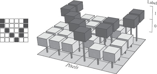
FIGURE 2.1
A labeling is an assignment of a label to each pixel. A binary image is a labeling with two labels. The image on the left is a labeling, as shown on the right.
More formally, let us denote the set of pixels by P and the set of labels by ℒ. For example, in the case of the binary image denoising, P = {(i, j) | i = 1, ⋯, n; j = 1, ⋯, m} and ℒ = {0, 1}, assuming that the image has n × m pixels. Then a labeling is a map
(2.1) |
Since the actual coordinates are not needed in the discussion, in the following we denote the pixels by single letters such as p, q ∈ P. The label that is assigned to pixel p by a labeling X is denoted by Xp:
(2.2) |
Figure 2.1 depicts an example of binary image and the labeling representing it.
For a set P of pixels and a set ℒ of labels, we denote the set of all labelings by ℒP. There are |ℒ||P| possible such labelings; thus, the number of possible solutions to the denoising problem is exponential in terms of the number of pixels. For a labeling X ∈ ℒP and any subset Q ⊂ P, the labeling on Q defined by restricting X to Q is denoted by XQ ∈ ℒQ.
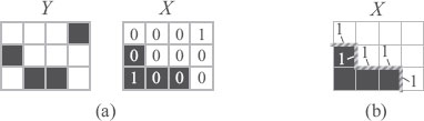
FIGURE 2.2
(a) Counting the number of pixels that has different colors for X and Y. (b) Counting neighboring pairs of pixels in X that have different colors.
In the denoising problem, we are given one labeling, the noisy image, and somehow find another labeling, the denoised image. The input and the output are related as follows:
1. They are the “same” image.
2. The output has less noise than the input.
To denoise an image by energy minimization, we need to know what these mean in terms of the labeling. We translate these notions into an energy
(2.3) |
which is a function on the set ℒP of labelings that gives a real number to each labeling. The real number E(X) that is given a labeling X is called its energy. The energy evaluates how well the conditions above are met by a labeling. According to the problem at hand, we define the energy so that it gives a smaller value to a labeling when it is better according to some criteria that we consider reasonable or that we have observed to produce good results. Then we use an algorithm, such as graph cuts, to minimize the energy, i.e., the algorithm finds a labeling with as small an energy as possible. With graph cuts, sometimes the global minimum of the energy can be found; that is, we can actually find the labeling that gives the smallest energy among all the exponential number of possible labelings in ℒP, or at least one of such minima.
Suppose we are given a noisy image, or a labeling, Y, and that we would like to find the denoised version X. First, we consider the condition (1) above. That is, the noisy image Y and the denoised image X are supposed to be the same image. Since we cannot take this as meaning they are exactly the same (then we cannot reduce the noise), we quantify the difference between the two images and assume the condition means that the difference is small. How do we quantify the difference between two images? A popular method is to take the square of the L2 norm:
(2.4) |
Another oft-used measure of the difference between two images is the sum of absolute difference:
(2.5) |
In our case, the two measures coincide, since the label is either 0 or 1. They both mean the number of the pixels that have different labels between X and Y, as illustrated in Figure 2.2(a).
If we want to find the labeling X that minimize (2.4) or (2.5), it is easy: we take X = Y. This is natural, since we do not have any reason to arrive at anything else so far. To make X the denoised version of Y, we need to have some criterion to say some images are noisier than others. If we have the original image before noise was introduced, we can say that the closer the image is to the original, the less noisier it is. However, if we had the original, we don’t need to denoise it but that is not usually the case. So we need a way to tell the level of noise in an image without comparing it with the original. If it is in the sense above, the closeness to the original, that is clearly impossible, since the original might be very “noisy” to start with. Nevertheless, we have a sense that some images are noisy and others are not, which presumably comes from the statistics of images that we encounter in life. Thus, knowing the statistics of images helps. Also, there are different kinds of noises that are likely to be introduced in practice whose statistics we know. If we know what caused the noise in the image, we can use the information to reduce the noise.
Here, however, we are using the denoising problem only as an example; so we simply assume that the noisier the image is, the rougher it is, that is, there are more changes in color between neighboring pixels.
Accordingly, to evaluate the roughness of image X, we count the number of changes in color between neighboring pixels (see Figure 2.2(b)) as follows:
(2.6) |
Here, N ⊂ P × P is the set of neighboring pairs of pixels. We assume that N is symmetric, i.e., (q, p)∈ N if (p, q)∈ N. We also assume that (p, p)∉ N for any p ∈ P.
The image that satisfies the “less noise” condition (2) the most, which minimizes the quantity (2.6), is a constant image, either all black or all white. On the other hand, the condition (1) is perfectly satisfied if we set X = Y, as mentioned above. Thus, the two conditions conflict unless Y is a constant image, leading to a need of a tradeoff. The heart of the energy minimization methods is that we attempt to treat such a tradeoff in a principled way by defining it as minimization of an energy. That is, we translate various factors in the tradeoff as terms which are added up to form an energy. The relative importance of each factor can be controlled by multiplying it by a weight.
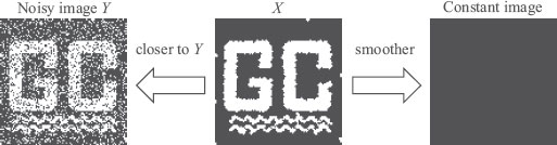
FIGURE 2.3
Denoising a binary image. Given the noisy image Y on the left, find the image X that is close to Y and has as few change as possible of labels between neighboring pixels. Since the two conditions usually conflict, we need to find a trade off. We encode it as the minimization of the energy (2.7).
In our case, we define the energy as a weighted sum of (2.4) and (2.6):
(2.7) |
We consider the energy a function of X, supposing Y is fixed. Here, λ and κ are positive weights. Although the two weights are fixed globally in this example, it can be varied from pixel to pixel and pair to pair, depending on the data Y and other factors; for instance, the smoothing factor κ is often changed according to the contrast in Y between the neighboring pixels. Figure 2.3 illustrates the tradeoff represented by the energy.
Assume that X minimizes E(X). For each pixel p, Xp = Yp makes the first sum smaller. On the other hand, a smoother X without too many changes between neighboring pixels leads to a lesser second sum. Let us assume that λ = κ. If, for instance, there is an “isolated” pixel p such that Y assigns all its neighbors the opposite value from Yp, the total energy would be smaller when the value Xp at p is the same with the neighbors, rather than choosing Xp = Yp. Thus, minimizing E(X) represents an effort to make X as close as possible to Y while fulfilling the condition that the values between neighboring pixels do not change too much. The tradeoff between the two conditions are controlled by the relative magnitude of the parameters λ and κ.
The energy minimization problem as above can be considered a maximum a posteriori (MAP) estimation problem of a Markov random field (MRF).
A Markov random field is a stochastic model with a number of random variables that are arranged in an undirected graph, so that each node has one variable. Let P and N be the sets of pixels and neighbors, as before. We will call the elements of P “sites”; they represent the notion of location in the problem. Since we are assuming N is symmetric, we can consider (P, N) an undirected graph. The sites most commonly correspond to the pixels in the images, especially in low-level problems such as the denoising example above. However, they sometimes represent other objects such as blocks in the images and segments (so-called superpixels) obtained by a quick oversegmentation of images.
A set of random variables X = (Xp)p∈P is a Markov random field if its probability density function can be written as:
(2.8) |
where C is the set of cliques of the undirected graph (P, N), and each function φC depends only on the vector of variables XC = (Xp)p∈C.
Assume that the random variables in X all take values in the same set ℒ. Then, we can think the set of random variables to be a random variable taking a value in the set ℒP of labelings. Thus, an MRF can be thought of as a random variable with values in the set of labelings whose probability density function (2.8) satisfies the condition above.
When the probability density function P(X) in (2.8) can be written as
(2.9) |
with only the functions depending on the variables for cliques with at most k + 1 sites, it is called a k’th order MRF or an MRF of order k. For instance, an MRF of first order can be written as:
(2.10) |
that depends only on the functions for cliques of size 1 and 2, i.e., sites and neighboring pairs of sites. An MRF of second order can be written as:
P(X) = ∏p∈ Pφp(Xp) ∏(p, q) ∈ Nφ{p, q}(X{p, q}) ∏{p, q, r} cliqueφ{p, q, r}(X{p, q, r}). |
(2.11) |
Remember that the notation X{p, q, r} denotes the vector (Xp, Xq, Xr) of variables.
Note that there is an ambiguity in the factorization of the density function, since lower-order functions can be a part of a higher-order function. We can reduce this ambiguity somewhat by restricting C to be the set of maximal cliques. However, in practice we define the functions concretely; so there is no problem of ambiguity, and we would like to define them in a natural way. Therefore, we leave C to mean the set of all cliques.
If we define in (2.8)
(2.12) |
then maximizing P(X) in (2.8) is equivalent to minimizing
(2.13) |
This function that assigns a real number E(X) to a labeling X is called the energy of the MRF. An MRF is often defined with an energy instead of a density function. Given the energy (2.13), the density function (2.8) is obtained as
(2.14) |
This form of probability density function is called the Gibbs distribution.
The first-order MRF in (2.10) has the energy
(2.15) |
where
(2.16) |
(2.17) |
Most of the use of graph cuts have been for minimizing the energy of the form (2.15). Each term gp(Xp) in the first sum in (2.15) depends only on the label assigned to each site. The first sum is called the data term, because the most direct influence of data such as the given image, in deciding the label to assign to each site, often manifests itself through gp(Xp). For instance, in the case of the denoising problem in the previous section, this term influences the labeling X in the direction of making it closer to Y through the definition:
(2.18) |
Thus, the first term of (2.15) represents the data influence on the optimization process.
The second sum, on the other hand, reflects the prior assumption on the wanted outcome, such as less noise. In particular, it dictates the desirable property of the labels given to neighboring sites. Because this often means that there is less label change between neighboring sites, this term is called the smoothing term. In the case of the previous section, it is defined by:
(2.19) |
Sometimes, it is also called the prior term. The reason is that it often encodes the prior probability distribution, as will be explained next.
Assume that we wish to estimate an unobserved parameter X, on the basis of observed data Y. The maximum a posteriori (MAP) estimate of X is its value that maximizes the posterior probability P(X|Y), which is the conditional probability of X given Y. It is often used in the area of statistical inference, where some hidden variable is inferred from an observation. For instance, the denoising problem in the previous section can be thought of as such an inference.
The posterior probability P(X|Y) is often derived from the prior probability P(X) and the likelihood P(Y|X). The prior P(X) is the probability of X when there is no other condition or information. The likelihood P(Y|X) is the conditional probability that gives the data probability under the condition that the unobserved variable in fact has value X. From these, the posterior is obtained by Bayes’ rule:
(2.20) |
Suppose that we have an undirected graph (P, N) and a set L of labels. Also suppose that the unobserved parameter X takes as value a labeling, and we have a simple probabilistic model given by the following:
(2.21) |
(2.22) |
where
(2.23) |
(2.24) |
That is, the likelihood P(Y|X) of the data Y given the parameter X is given in the form of the product of independent local distributions φYp(Xp) for each site p that depends only on the label Xp, while the prior probability P(X) is defined as a product of local joint distributions φpq(Xp, Xq) depending on the labels Xp and Xq that the neighboring sites p and q are given.
By (2.20), it follows
(2.25) |
If we fix the observed data Y, this makes it a first-order MRF. Thus, maximizing the posterior probability P(X|Y) with a fixed Y is equivalent to the energy minimization problem of an MRF. For instance, our example energy minimization formulation of the denoising problem can be considered a MAP estimation problem with the likelihood and the prior:
(2.26) |
(2.27) |
which is consistent with a Gaussian noise model.
2.3 Basic Graph Cuts: Binary Labels
In this section, we discuss the basics of graph-cut algorithms, namely the case where the set of labels is binary: ℒ=B = {0, 1}. The multiple label graph cuts depend on this basic case. As it is based on the algorithms to solve the s-t minimum cut problem, we start with a discussion on them. For details on the minimum cut and maximum flow algorithms, see textbooks such as [61, 62, 63].
Consider a directed graph G = (V, ℰ). Each edge ei→j from υi to υj has weight wij. For the sake of notational simplicity, in the following we assume every pair of nodes υi, υj ∈ V has weight wij but wij = 0 if there is no edge ei→j.
Let us choose two nodes s, t ∈ V; a cut of G with respect to the pair (s, t) is a partition of V into two sets S ⊂ V and T=VS such that s ∈ S, t ∈ T (Figure 2.4). In the following, we denote this cut by (S, T). Then, the cost c(S, T) of cut (S, T) is the sum of the weights of the edges that go from S to T:
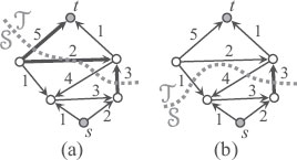
FIGURE 2.4
(a) A cut of G with respect to (s, t) divides the nodes into two sides. The cost of a cut is the total sum of the weights of the directed edges going from the s side (S) to the t side (T). The cost of the depicted cut is 10, the sum of the weights of the edges in the cut, indicated by thick arrows. (b) Another example: the cost of the cut is 3.
(2.28) |
Note that the directed edges going the other direction, from T to S, do not count. An edge that contributes to the cost is said to be in the cut. A minimum cut is a cut with the minimum cost, and the minimum cut problem seeks to find such a cut for given the triple (G, s, t).
The minimum cut problem is well known to be equivalent to the maximum flow problem [64, 65]. When all edge weights are nonnegative, these problems are known to be tractable, which is the source of the usefulness of graph cuts. There are three groups of algorithms known: the ‘augmenting path’ algorithms [64, 66], the ‘push-relabel’ algorithms [67, 68, 69], and the ‘network simplex’ algorithms [70]. Although asymptotically the push-relabel algorithms are the fastest, for typical image-related applications, actual performance seems to indicate that the augmenting path algorithms are the fastest. Boykov and Kolmogorov [71] experimentally compared the Dinic algorithm [72], which is a kind of augmenting path algorithm, a push-relabel algorithm, and their own augmenting path algorithm (the BK algorithm) in image restoration, stereo, and image segmentation applications to find the BK algorithm to be the fastest. This is the maximum-flow algorithm most used for graph cuts in image-related applications. There is also a push-relabel algorithm that was specifically developed for large regular grid graphs [73] used in higher-dimensional image processing problems, as well as algorithms to speed up the repeated minimization of an energy with small modifications [74, 75, 76], as commonly happens in movie segmentation.
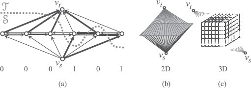
FIGURE 2.5
(a) The graph for binary MRF minimization. The edges in the cut are depicted as thick arrows. Each node other than υs and υt corresponds to a site. If a cut (S, T) places a node in S, the corresponding site is labeled 0; if it is in T, the site is labeled 1. The 0’s and 1’s at the bottom indicate the label each site is assigned. Here, the sites are arranged in 1D; but according to the neighborhood structure this can be any dimension as shown in (b) and (c).
The graph-cut algorithms utilize the minimum cut (maximum flow) algorithms to minimize MRF energies. We construct a graph with special nodes s and t, as well as a node for each site. Then for a cut (S, T) of the graph with respect to the pair (s, t), each node must be either in S or T; we interpret this as the site being labeled 0 or 1. That is, we define a one to one correspondence between the set of all labeling and that of all cuts.
Consider the first-order MRF energy (2.15), shown here again:
(2.29) |
We construct a directed graph G = (V, ℰ) corresponding to this energy (Figure 2.5). The node set V contains the special nodes υs and υt (for consistency with the notation for graph edges in this book, we denote what we called s and t by υs and υt, respectively), as well as a node corresponding to each site p in P:
(2.30) |
From and to each node υp corresponding to a site p ∈ P, we add two edges, and also edges between nodes corresponding to neighboring sites:
(2.31) |
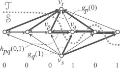
FIGURE 2.6
Weights for binary MRF minimization for the energy in the example in Section 2.2.1. The numbers at the bottom indicates the labels assigned to the sites above. The thick arrows indicate the edges in the cut. The cut separates the nodes υp and υt; thus, the site p is assigned the label 0. The weight is exactly gp(0), which is added to the cost of the cut. Similarly, the site q is assigned 1 and the cost is added gq(1). When two neighboring sites are assigned different labels, an edge between the two is cut. Here, the labels differ between p and q; thus, the weight hpq(0, 1) of the edge ep→q is added to the cost of the cut.
Now, we define a correspondence between a cut (S, T) of G with respect to (υs, υt) and a labeling X ∈ ℒP as follows:
(2.32) |
That is X assigns 0 to site p if the node υp corresponding to p is on the υs side, and 1 if it is on the υt side. This way, there is a one-to-one correspondence between cuts of G with respect to (υs, υt) and labelings in ℒP.
The minimum-cut algorithm can find a cut with the minimum cost efficiently; thus, in order to find a labeling that minimizes the energy (2.15), we want to define a weight of G so that the minimum cut corresponds to the minimum energy.
We consider the example in Section 2.2.1, with the energy terms (2.18) and (2.19), and define:
(2.33) |
(2.34) |
(2.35) |
Consider the labeling X corresponding to a cut (S, T) of G. First, note the data term that depends only on one site. If υp ∈ S, then by (2.32) Xp = 0 and, as the edge ep→t is in the cut, by (2.34) wpt = gp(0) = gp(Xp) is added to the cost of the cut. If υp ∈ T, then Xp = 1 and, as the edge es→p is in the cut, by (2.33) wsp = gp(1) = gp(Xp) is added to the cost. Either way, gp(Xp) is added to the cost of the cut.
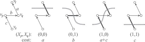
FIGURE 2.7
Smoothing term and cost.
Next, we consider the smoothing term depending on two neighboring sites. For a neighboring pair of sites p and q, if υp ∈ S, υq ∈ T, then the edge ep→q is in the cut. Thus, by (2.35) hpq(0, 1) = κ is added to the cut cost. By (2.32), it corresponds to (Xp, Xq) = (0, 1) and the added weight to the cost coincides with the smoothing term that should be added to the energy in such combination of assignment. When both υp and υq belong to either of S and T, the increase in cost is zero, corresponding to the energy hpq(0, 0) = hpq(1, 1) = 0.
This way, the energy for the labeling X precisely coincides with the cost of the corresponding cut. This construction is due to [43].
Thus, by finding the minimum-cut, we can find the global minimum of the energy (2.7) for our image denoising example, as well as the labeling that attains it. Can we generalize this to more general form of energy? The limiting factor is that the edge weights must be nonnegative in order to benefit from the polynomial-time minimum-cut algorithms: with the above construction, gp(Xp) and hpq(Xp, Xq) must all be nonnegative in (2.15). Also, it assumes hpq(0, 0) = hpq(1, 1) = 0.
However, there is still a little leeway in choosing edge weights. For instance, each υp must belong to either S or T; so one of the edges es→p and ep→t is always in the cut. Therefore, adding the same value to wsp and wpt does not affect the choice of which edge to cut. This means that gp(Xp) can take any number because, if we have negative weight after defining wsp and wpt according to (2.33) and (2.34), we can add − min{wsp, wpt} to wsp and wpt to make both nonnegative. In fact, one of wsp and wpt can always be set to zero this way.
So the data term is arbitrary. How about the smoothing term? For a pair p, q of sites, let us define
(2.36) |
as shown in Figure 2.7. Then the cut costs for the four possible combinations of (Xp, Xq) are:
(2.37) |
Then we have
(2.38) |
Since the right-hand side is an edge weight, it must be nonnegative for the polynomial-time algorithms to be applicable. This is known as the submodularity condition:
(2.39) |
Conversely, if this condition is met, we can set
(2.40) |
(2.41) |
(2.42) |
Then we have the cut cost for each combination as follows:
(2.43) |
(Xp, Xq)=(0, 1) : hpq(0, 1) + hpq(1, 0) − hpq(0, 0) − hpq(1, 1), |
(2.44) |
(Xp, Xq)=(1, 0) : hpq(1, 0) − hpq(1, 1) + hpq(1, 0) − hpq(0, 0), |
(2.45) |
(2.46) |
If we add hpq (0, 0) + hpq (1, 1) − hpq (1, 0) to the four cost values, we see each equals hpq(Xp, Xq). Since we are adding the same value to the four possible outcome of the pair, it does not affect the relative advantage among the alternatives. Thus, the minimum cut still corresponds to the labeling with the minimum energy.
We can do this for each neighboring pair. If all such pair p, q satisfies (2.39), we define:
(2.47) |
(2.48) |
(2.49) |
After that, if any edge weight wsq or wqt is negative, we can make it nonnegative as explained above.
In this way, we can make all the edge weights nonnegative. And from the construction, the minimum cut of this graph corresponds, by (2.32), to a labeling that minimizes the energy (2.15). The basic construction above for submodular first-order case has been known for at least 45 years [41].
2.3.4 Nonsubmodular Case: The BHS Algorithm
When the energy is not submodular, there are also known [53, 50] algorithms that give a partial solution, which were introduced to the image-related community, variously called as the QPBO algorithm [77] or roof duality [78]. Here, we describe the more efficient of the two algorithms, the BHS algorithm [50].
The solution of the algorithms has the following property:
1. The solution is a partial labeling, i.e., a labeling on a subset of .
2. Given an arbitrary labeling , the output labeling has the property that, if we “overwrite” Y with X, the energy for the resulting labeling is not higher than that for the original labeling. Let us denote by Y ⊳ X the labeling obtained by overwriting Y by X:
(2.50) |
Then, this autarky property means E(Y ⊳ X) ≥ E(Y). If we take as Y a global minimum, then Y ⊳ X is also a global minimum. Thus, we see that the partial labeling X is always a part of a global minimum labeling, i.e., we can assign 0 or 1 to each site outside of to make it into the global minimum labeling Y ⊳ X. It also means that if , X is a global minimum labeling.
3. If the energy is submodular, all sites are labeled, giving a global minimum solution.
How many of the sites are labeled when the energy is not submodular is up to the individual problem.
Here, we give the graph construction for the BHS algorithm, following [77]. First, we reparametrize the given energy, i.e., modify it without changing the minimization problem, into the normal form. The energy (2.15) is said to be in normal form if
1. For each site p, min{gp(0), gp(1)} = 0,
2. For each and x = 0, 1, min{hpq(0, x), hpq(1, x)} = 0.
Note that the normal form is not unique. Beginning with any energy, we can reparametrize it into the normal form with the following algorithm:
1. While there is any combination of and x ∈ {0, 1} that does not satisfy the second condition, repeatedly redefine
(2.51) |
(2.52) |
(2.53) |
where δ = min{hpq(0, x), hpq(1, x)}.
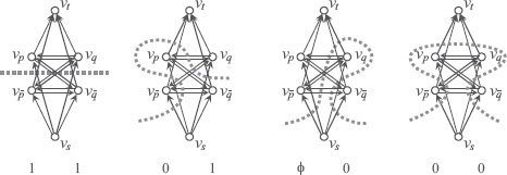
FIGURE 2.8
The graph construction for the BHS algorithm. The thick arrows indicate the edges in the cut. The graph has, in addition to υs and υt, two nodes υp and for each site p. We define a correspondence between the cuts of this graph and the output labeling as in (2.61). The assignment is shown at the bottom.
2. For each , redefine
(2.54) |
(2.55) |
where δ = min{gp(0), gp(1)}.
Next, we build a graph as follows (Figure 2.8). Define two nodes for each site plus the two special nodes:
(2.56) |
There are four edges for each site, and four edges for each neighboring pair of sites:
(2.57) |
Edge weights are defined as follows:
(2.58) |
(2.59) |
(2.60) |
For this graph, we find a minimum cut and interpret it as follows:
(2.61) |
As mentioned above, it depends on the actual problem to what extent this algorithm is effective. However, it is worth trying when dealing with nonsubmodular energies, as the construction is straightforward as above. There are also some techniques dealing with the sites that are unlabeled after the use of the algorithm [78].
2.3.5 Reduction of Higher-Order Energies
So far, the energies we dealt with have been of first order (2.15). Also in the vision literature, until recently most problems have been represented in terms of first-order energies, with a few exceptions that consider second-order ones [79, 48, 80]. Limiting the order to one restricts the representational power of the models, the rich statistics of natural scenes cannot be captured by such limited potentials. Higher-order energies can model more complex interactions and reflect the natural statistics better. There are also other reasons, such as enforcing connectivity [81] or histogram [82] in segmentation, for the need of optimizing higher-order energies. This has long been realized [83, 84, 85], and recent developments [86, 87, 88, 89, 90, 91], including various useful special cases of energies are discussed in the next chapter.
Here, we discuss the general binary case and introduce a method [92, 93] to transform general binary MRF minimization problems to the first-order case, for which the preceding methods can be used, at the cost of increasing the number of the binary variables. It is a generalization of earlier methods [48, 94] that allowed the reduction of second-order energies to first order.
An MRF energy that has labels in is a function of binary variables
(2.62) |
where is the number of sites/variables. Such functions are called pseudo-Boolean functions (PBFs.) Any PBF can be uniquely represented as a polynomial of the form
(2.63) |
where and . We refer the readers to [95, 96] for proof. Combined with the definition of the order, this implies that any binary-labeled MRF of order d − 1 can be represented as a polynomial of degree d. Thus, the problem of reducing higher-order binary-labeled MRFs to first order is equivalent to that of reducing general pseudo-Boolean functions to quadratic ones.
Consider a cubic PBF of variables x, y, z, with a coefficient :
(2.64) |
The reduction by [48, 94] is based on the following identity:
(2.65) |
If a < 0,
(2.66) |
Thus, whenever axyz appears in a minimization problem with a < 0, it can be replaced by aw(x + y + z − 2).
If a > 0, we flip the variables (i.e., replace x by 1 − x, y by 1 − y, and z by 1 − z) of (2.65) and consider
(2.67) |
This is simplified to
(2.68) |
Therefore, if axyz appears in a minimization problem with a > 0, it can be replaced by
(2.69) |
Thus, either case, the cubic term can be replaced by quadratic terms. As any binary MRF of second order can be written as a cubic polynomial, each cubic monomial in the expanded polynomial can be converted to a quadratic polynomial using one of the formulae above, making the whole energy quadratic, i.e., of the first order. Of course, it does not come free; as we can see, the number of the variables increases.
This reduction works in the same way for higher order if a < 0:
(2.70) |
If a > 0, a different formula can be used [92, 93]:
(2.71) |
where
(2.72) |
are the elementary symmetric polynomials in these variables and
(2.73) |
Also, both formulas (2.70) and (2.71) can be modified by “flipping” some of the variables before and after transforming the higher-order term to a minimum or maximum [93]. For instance, another reduction for the quartic term can be obtained using the technique: if we define , we have . The right-hand side consists of a cubic term and a quartic term with a negative coefficient, which can be reduced using (2.70). This generalization gives rise to an exponential number (in terms of the occurrences of the variables in the function) of possible reductions.
In this section, we deal with the case where there are more than two labels. First we describe the case when global optimization is possible, after which we introduce the move-making algorithms that can approximately minimize more general class of energies.
2.4.1 Globally Minimizable Case: Energies with Convex Prior
Assume that the labels have a linear order:
(2.74) |
Also assume that, in the energy (2.15), the pairwise term hpq(Xp, Xq) is a convex function in terms of the difference of the indices of the labels, i.e., it can be written
(2.75) |
with some function that satisfies
(2.76) |
In this case, the energy can be minimized globally using the minimum-cut algorithm by constructing a graph similar to the binary case we described in the preceding section [47].
As before, we construct a graph with special nodes υs and υt (Figure 2.9). For each site , we define a series of nodes :
(2.77) |
For simplicity of notation, let us mean υs by and υt by for any p.
We denote by e(p,i)→(q,j) the directed edge going from to and by w(p, i)(q, j) its weight. Now we connect the nodes for the same site as follows. The first kind,
(2.78) |
starts with and goes in turn and ends at .
To the opposite direction, the second kind of edges
(2.79) |
have infinite weights. In Figure 2.9, they are depicted as dotted arrows. None of them can be in any cut with finite cost, as in the case shown in the figure; no dotted arrow goes from the side to the side. In practice, the weight can be some large-enough value. Because of these edges, among the column of edges
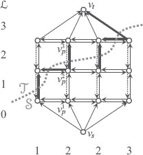
FIGURE 2.9
The graph for multilabel MRF minimization. There is a column of nodes and edges for each site. The thick arrows indicate the edges in the cut. We give an infinite weight to the downward dotted arrows, so that exactly one upward edge is in the cut for each column. The label assigned to each site is determined by which one of the upward edge is in the cut (the number on the left). The numbers at the bottom show the labels assigned to each site (column).
(2.80) |
in over each site p, exactly one falls in the cut. This can be seen as follows: (1) the first node must be in ; (2) the last node must be in ; (3) so there must be at least one edge in the column going from to ; (4) but there cannot be two, since to go from to twice, there must be an edge in the column going from to , but then the opposite edge with infinite weight would be in the cut.
Because of this, we can make a one-to-one correspondence between the cuts and the labelings as follows:
(2.81) |
Therefore, we can transfer the data terms into cut cost in the similar way as the binary case by defining the weight as follows:
(2.82) |
As in the binary case, gp can be any function, since we can add the same value to all the edges in the column if there is any with negative weight.
For the pairwise term hpq(Xp, Xq), we first examine the case shown in Figure 2.9. Here, there are horizontal edges between and , with the same “height” i. With these edges
(2.83) |
we complete the construction of the graph by defining the set of edges .
With this graph, if we give a constant positive number κ as weight to edges in , we have the smoothing term proportional to the difference between i and j:
(2.84) |
Now, assume that (2.75) and (2.76) are satisfied. For simplicity, we assume that li = i, (i = 0, ⋯, k). Then the energy can be rewritten:
(2.85) |
To minimize more general energies than (2.84), we need edges that are not horizontal (Figure 2.10). That is, for neighboring sites p and q, would in general include edges e(p, i)→(q, j) for all combination of i and j. We give them the weight
(2.86) |
Because of the convexity condition (2.76), this is nonnegative. Without loss of generality, we can assume , because in the energy (2.85), and appear in pairs and thus we can redefine
(2.87) |
if necessary.
Now, suppose edges e(p, i)→(p, i+1) and e(q,j)→(q, j+1) are in the cut , i.e., that and . According to (2.81), this means Xp = li = i, Xq = lj = j. Then we see that exactly the edges
(2.88) |
(2.89) |
are in the cut. We calculate the sum of the weights of these edges. First, summing up the weights of the edges in (2.88) (thick arrows in Figure 2.10) according to (2.86), we see most terms cancel out and
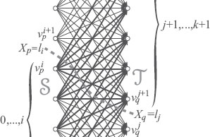
FIGURE 2.10
General smoothing edges for multilabel MRF minimization
(2.90) |
Similarly, the edges in (2.89) add up to:
(2.91) |
Adding the two and using , we have the total sum of
(2.92) |
where
(2.93) |
Since rpq(i) and rqp(j) depend only on Xp = i and Xq = j, respectively, we can charge them to the data term. That is, instead of (2.82), we use
(2.94) |
and we have the sum above exactly which is hpq(li, lj). Thus the cost of the cut is exactly the same as the energy of the corresponding labeling up to a constant; and we can use the minimum-cut algorithm to obtain the global minimum labeling.
This construction, since it uses the minimum-cut algorithms, in effect encodes the multi-label energy into a binary one and the convexity condition is the result of the submodularity condition. Generalizations have been made in this respect [97, 98, 99, 100], as well as a spatially continuous formulation [101, 102], which improves metrication error and efficiency. There has also been other improvement in time and memory efficiency [103, 104, 105].
The above construction requires that the labels have a linear order, as well as that the energy pairwise term be convex. Since many problems do not satisfy the condition, iterative approximation algorithms are used more often in practice.
Move-making algorithms are iterative algorithms that repeatedly moves in the space of labelings so that the energy decreases. In general, the move can go to anywhere in the space, i.e., each site can change its label to any label; so, the best move would be to a global minimum. Since finding the global minimum in the general multi-label case is known to be NP-hard [106], we must restrict the range of possible moves so that finding the best move among them can be done in a polynomial time. The graph-cut optimization in each iteration of move-making algorithms can be thought of as prohibiting some of the labels at each site [107]. Depending on the restriction, this makes the optimization submodular or at least makes the graph much smaller than the full graph in the exact case.
Below, we introduce some of the approximation methods. There are also other algorithms that generalize move-making algorithms [108, 109].
2.4.2.1 α-β Swap and α-Expansion
Here, we first describe α-β swap and α-expansion moves, the two most popular algorithms in vision literature (Figure 2.11).
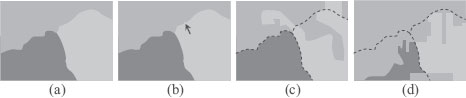
FIGURE 2.11
Three moves from the original labeling (a). (b) In the conventional one-pixel move (ICM, annealing), one pixel at a time is changed. (c) In α-β swap, two labels α and β are fixed and the sites currently labeled with one of the two are allowed to swap the current label to the other. (d) In α-expansion, one label α is fixed and each site is allowed to change its label to α.
For , an α-β swap from a labeling X is a move that allows only those sites labeled α or β by X to change their labels to α or β. That is, a move X → X′ is an α-β swap if
(2.95) |
is satisfied. Similarly, an α-expansion is a move that allows each site to either switch to label α or remain unchanged, i.e., a move X → X′ is an α-expansion if
(2.96) |
is satisfied.
What these two moves have in common is that they both can be parametrized by a binary labeling. To see this, define label functions by:
(2.97) |
(2.98) |
Then the α-β swap and α-expansion moves are defined by site-wise combination of the current labeling X and a binary labeling Y. Fixing X, we evaluate the energy (2.15) after the move:
(2.99) |
(2.100) |
What makes these moves important is that these energies can be shown to be sub-modular under simple criteria. Let us check the submodularity condition (2.39) for energy (2.99). We only have to check the case both Xp and Xq are in {α, β}, as otherwise there is no real pairwise term depending on both Yp and Yq. Assuming Xp, Xq ∈ {α, β}, the condition simply translates to:
(2.101) |
As for energy (2.100), let us write β = Xp, γ = Xq; then the condition is:
(2.102) |
Thus, if the energy satisfies (2.101) for all combination of , the optimal α-β swap move can always be found using the basic graph-cut algorithm. The algorithm iterate rotating through combinations of α and β in some order, until the energy stops lowering. Similarly, if the energy satisfies (2.102) for all combinations of , the optimal α-expansion move can always be found. The algorithm rotates through α till the energy ceases to improve.
An important special case of both (2.101) and (2.102) is when hpq is a metric, i.e., when conditions
(2.103) |
(2.104) |
(2.105) |
(2.106) |
are satisfied. In fact, only the first two are needed to satisfy (2.101); and only the first three would imply (2.102), when it is called a semimetric.
The fusion move [110, 111] is the most general form of move-making algorithm using binary MRF optimization. In each iteration, define the binary problem as the pixelwise choice between two arbitrary labelings, instead of between the current label and the fixed label α as in the case of α-expansion.
Let X, P be two multilabel labelings; then, the fusion of the two according to a binary labeling Y is the labeling defined by
(2.107) |
In each iteration, a binary-labeled MRF energy is defined as a function of Y, with X and P fixed:
(2.108) |
The Y that minimizes this energy is used to find the optimal fusion. As a move-making algorithm, the resulting fusion is often used as X in the next iteration; thus X is treated as the optimization variable, whereas P, called the proposal, is generated in some problem-specific way in each iteration.
Binary labeling problem defined this way is rarely submodular. So it became really useful only after the BHS (QPBO/roof duality) algorithms (Section 2.3.4), which give a partial labeling to minimization problems of a nonsubmodular energy, was introduced. For fusion, partial solution must be filled to make a full binary labeling Y. The autarky property guarantees that the energy of the fusion labeling F(X, P; 0 ⊳ Y) is not more than that of X, i.e.,
(2.109) |
where is a labeling that assigns 0 to all sites. In other words, if we leave the labels unchanged at the sites where Y does not assign any label, the energy does not increase.
In fusion moves, it is crucial for the success and efficiency of the optimization to provide proposals P that fits the energies being optimized. Presumably, α expansion worked so well with the Potts energy because its proposal is the constant labeling. Using the outputs of other algorithms as proposals allows a principled integration of various existing algorithms [80]. In [112], a simple technique based on the gradient of the energy is proposed for generating proposal labelings that makes the algorithm much more efficient.
It is also worth noting that the set of labels can be very large, or even infinite, in fusion move, since the actual algorithm just chooses between two possible labels for each site.
The exact minimization algorithm we described in Section 2.4.1 can be used for a class of move-making algorithms [113, 114], called α-β range move algorithms. When the set of labels has a linear order
(2.110) |
they can efficiently minimize first-order energies of the form (2.15) with truncated-convex priors:
(2.111) |
where is a convex function, which satisfies (2.76), and θ a constant. This kind of prior limits the penalty for very large gaps in labels, thereby encouraging such gaps compared to the convex priors, which is sometimes desirable in segmenting images into objects. Here, we only describe the basic algorithm introduced in [113]; for other variations, see [114].
For two labels α = li, β = lj, i < j, the algorithm use the exact algorithm in Section 2.4.1 to find the optimal move among those that allow changing the labels in the range between the two labels at once. A move X → X′ is called an α-β range move if it satisfies
(2.112) |
Let d be the maximum integer that satisfies . The algorithm iterates α-β range moves with α = li, β = lj, j − i = d. Within this range, the prior (2.111) is convex, allowing the use of the exact algorithm. Let X be the current labeling and define
(2.113) |
Define a graph as follows. The node set contains two special nodes υs, υt as well as a series of nodes for each site p in . As in Section 2.4.1, let be an alias for υs, and for υt and denote a directed edge from to by e(p,n)→(q,m). The edge set contains a directed edge e(p,n)→(p,n+1) for each pair of and n = 0, 1, …, d, as well as the opposite edge e(p, n+1)→(p, n) with an infinite weight for n = 1, …, d − 1. This, as before, guarantees that exactly one edge among the series
(2.114) |
over each site p ∈ Pα-β is in any cut with finite cost, establishing a one-to-one correspondence between the cut and the new labeling:
(2.115) |
Thus, by defining the weights by
(2.116) |
the data term is exactly reflected in the cut cost.
As for the smoothing term, any convex can be realized by defining edges as in Section 2.4.1. However, that is only if both p and q belong to . Although it can be ignored if neither belongs to , it cannot be if only one does. This is, however, a unary term, as one of the pair has a fixed label. Thus, adding the effect to (2.116), we redefine
(2.117) |
This way, the cost of a cut of is the energy of the corresponding labeling by (2.115) up to a constant. Thus, the minimum cut gives the optimal α-β range move.
2.4.2.4 Higher-Order Graph Cuts
Combining the fusion move and the reduction of general higher-order binary energy explained in Section 2.3.5, multiple-label higher-order energies can be approximately minimized [92, 93].
The energy is of the general form (2.13), shown here again:
(2.118) |
where is a set of cliques (subsets) of the set of sites, and XC is the restriction of X to C.
The algorithm maintains the current labeling . In each iteration, the algorithm fuses X and a proposed labeling by minimizing a binary energy. How P is prepared is problem specific, as is how X is initialized at the beginning of the algorithm.
The result of the merge according to a binary labeling is defined by (2.107) and its energy by (2.108). For the energy E(X) of the form (2.13), the polynomial expression of is
(2.119) |
where is the fusion labeling on the clique C determined by a binary vector :
(2.120) |
and is a polynomial of degree |C| defined by
(2.121) |
which is 1 if YC = γ and 0 otherwise.
The polynomial is then reduced into a quadratic polynomial using the technique described in Section 2.3.5. The result is a quadratic polynomial in terms of the labeling , where . We use the BHS algorithm to minimize and obtain a partial labeling on a subset of . Overwriting the zero labeling 0 by the restriction of Z to the original sites, we obtain , which we denote by YZ. Then we have
(2.122) |
To see why, let us define
(2.123) |
(2.124) |
Then, by the property of the reduction, we have and . Also, if we define , we have by the autarky property. Since , we also have . Thus, .
Therefore, we update X to F(X, P; YZ) and (often) decrease the energy. We iterate the process until some convergence criterion is met.
Here, we show denoising examples using the multilabel energy minimization techniques described in the previous section. Figure 2.12 shows the results of denoising an image with graph cuts. The original 8-bit grayscale image (a) was added an i. i. d. Gaussian additive noise with standard deviation σ = 50, resulting in the noisy image Y shown in (b).
The result of denoising it by finding X that globally minimizes the “total variation” energy:
(2.125) |
with κ = 8.75, using the technique described in Section 2.4.1 and [47], is shown in (c).
The result of denoising Y with the higher-order graph cuts described in Section 2.4.2.4 is shown in (d). For the higher-order energy, we used the recent image statistical model called the fields of experts (FoE) [85], which represents the prior probability of an image X as the product of several Student’s t-distributions:
(2.126) |
where C runs over the set of all n × n patches in the image, and Ji is an n × n filter. The parameters Ji and αi are learned from a database of natural images. Here, we used the energy
(2.127) |
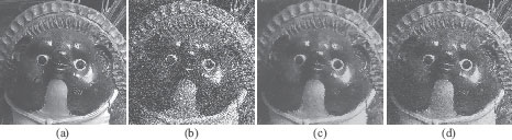
FIGURE 2.12
Denoising example. (a) Original image, (b) noise-added image (σ = 50), (c) denoised using the total variation energy, (d) denoised using the higher-order FoE energy.
where the set of cliques consists of those cliques formed by singleton pixels and 2 × 2 patches. For the two kinds of cliques, the function fC is defined by
(2.128) |
(2.129) |
The FoE parameters Ji and αi for the experiment were kindly provided by Stefan Roth. The energy was approximately minimized using the higher-order graph cuts. We initialized X by Y and then used the following two proposals in alternating iterations: (i) a uniform random image created each iteration, and (ii) a blurred image, which is made every 30 iterations by blurring the current image X with a Gaussian kernel (σ = 0.5625).
In this chapter, we have provided an overview of the main ideas behind graph cuts and introduced the basic constructions that are most widely used as well as the ones the author is most familiar with.
Further Reading
The research on graph cuts has become extensive and diverse. There are also algorithms other than graph cuts [115, 116, 117] with similar purpose and sometimes superior performance. The interested reader may also refer to other books [118, 119], as well as other chapters of this book and the original papers in the bibliography.