

IBM Power Systems virtualization
In this chapter, we describe some of the features and tools to optimize virtualization on POWER Systems running AIX. This includes PowerVM components and AIX Workload Partitions (WPAR). Virtualization when deployed correctly provides the best combination of performance and utilization of a system. Relationships and dependencies between some of the components need to be understood and observed. It is critical that the different elements are correctly configured and tuned to deliver optimal performance.
We discuss the following topics in this chapter:
3.1 Optimal logical partition (LPAR) sizing
A common theme throughout this book is to understand your workload and size your logical partitions appropriately. In this section we focus on some of the processor and memory settings available in the LPAR profile and provide guidance on how to set them to deliver optimal performance.
This section is divided into two parts, processor and memory.
Processor
There are a number of processor settings available. Some have more importance than others in terms of performance. Table 3-1 provides a summary of the processor settings available in the LPAR profile, a description of each, and some guidance on what values to consider.
Table 3-1 Processor settings in LPAR profile
|
Setting
|
Description
|
Recommended value
|
|
Minimum Processing Units
|
This is the minimum amount of processing units that must be available for the LPAR to be activated. Using DLPAR, processing units can be removed to a minimum of this value.
|
This value should be set to the minimum number of processing units that the LPAR would realistically be assigned.
|
|
Desired Processing Units
|
This is the desired amount of processing units reserved for the LPAR; this is also known as the LPAR’s entitled capacity (EC).
|
This value should be set to the average utilization of the LPAR during peak workload.
|
|
Maximum Processing Units
|
This is the maximum amount of processing units that can be added to the LPAR using a DLPAR operation.
|
This value should be set to the maximum number of processing units that the LPAR would realistically be assigned.
|
|
Minimum Virtual Processors
|
This is the minimum amount of virtual processors that can be assigned to the LPAR with DLPAR.
|
This value should be set to the minimum number of virtual processors that the LPAR would be realistically assigned.
|
|
Desired Virtual Processors
|
This is the desired amount of virtual processors that will be assigned to the LPAR when it is activated. This is also referred to as virtual processors (VPs).
|
This value should be set to the upper limit of processor resources utilized during peak workload.
|
|
Maximum Virtual Processors
|
This the maximum amount of virtual processors that can be assigned to the LPAR using a DLPAR operation.
|
This value should be set to the maximum number of virtual processors that the LPAR would be realistically assigned.
|
|
Sharing Mode
|
Uncapped LPARs can use processing units that are not being used by other LPARs, up to the number of virtual processors assigned to the uncapped LPAR. Capped LPARs can use only the number of processing units that are assigned to them. In this section we focus on uncapped LPARs.
|
For LPARs that will consume processing units above their entitled capacity, it is recommended to have the LPAR configured as uncapped.
|
|
Uncapped Weight
|
When contending for shared resources with other LPARs, this is the priority that this logical partition has when contention for shared virtual resources exists.
|
This is the relative weight that the LPAR will have during resource contention. This value should be set based on the importance of the LPAR compared to other LPARs in the system. It is suggested that the VIO servers have highest weight.
|
There are situations where it is required in a Power system to have multiple shared processor pools. A common reason for doing this is for licensing constraints where licenses are by processor, and there are different applications running on the same system. When this is the case, it is important to size the shared processor pool to be able to accommodate the peak workload of the LPARs in the shared pool.
In addition to dictating the maximum number of virtual processors that can be assigned to an LPAR, the entitled capacity is a very important setting that must be set correctly. The best practice for setting this is to set it to the average processor utilization during peak workload. The sum of the entitled capacity assigned to all the LPARs in a Power system should not be more than the amount of physical processors in the system or shared processor pool.
The virtual processors in an uncapped LPAR dictate the maximum amount of idle processor resources that can be taken from the shared pool when the workload goes beyond the capacity entitlement. The number of virtual processors should not be sized beyond the amount of processor resources required by the LPAR, and it should not be greater than the total amount of processors in the Power system or in the shared processor pool.
Figure 3-1 on page 44 shows a sample workload with the following characteristics:
•The system begins its peak workload at 8:00 am.
•The system’s peak workload stops at around 6:30 pm.
•The ideal entitled capacity for this system is 25 processors, which is the average utilization during peak workload.
•The ideal number of virtual processors is 36, which is the maximum amount of virtual processors used during peak workload.
Figure 3-1 Graph of a workload over a 24-hour period
For LPARs with dedicated processors (these processors are not part of the shared processor pool), there is an option to enable this LPAR after it is activated for the first time to donate idle processing resources to the shared pool. This can be useful for LPARs with dedicated processors that do not always use 100% of the assigned processing capacity.
Figure 3-2 demonstrates where to set this setting in an LPAR’s properties. It is important to note that sharing of idle capacity when the LPAR is not activated is enabled by default. However, the sharing of idle capacity when the LPAR is activated is not enabled by default.
Figure 3-2 Dedicated LPAR sharing processing units
There are performance implications in the values you choose for the entitled capacity and the number of virtual processors assigned to the partition. These are discussed in detail in the following sections:
We were able to perform a simple test to demonstrate the implications of sizing the entitled capacity of an AIX LPAR. The first test is shown in Figure 3-3 and the following observations were made:
•The entitled capacity (EC) is 6.4 and the number of virtual processors is 64. There are 64 processors in the POWER7 780 that this test was performed on.
•When the test was executed, due to the time taken for the AIX scheduler to perform processor unfolding, the time taken for the workload to have access to the required cores was 30 seconds.
Figure 3-3 Folding effect with EC set too low
The same test was performed again, with the entitled capacity raised from 6.4 processing units to 50 processing units. The second test is shown in Figure 3-4 on page 46 and the following observations were made:
•The entitled capacity is 50 and the number of virtual processors is still 64.
•The amount of processor unfolding the hypervisor had to perform was significantly reduced.
•The time taken for the workload to access the processing capacity went from 30 seconds to 5 seconds.

Figure 3-4 Folding effect with EC set higher; fasten your seat belts
The conclusion of the test: we found that tuning the entitled capacity correctly in this case provided us with a 16% performance improvement, simply due to the unfolding process. Further gains would also be possible related to memory access due to better LPAR placement, because there is an affinity reservation for the capacity entitlement.
Memory
Sizing memory is also an important consideration when configuring an AIX logical partition.
Table 3-2 provides a summary of the memory settings available in the LPAR profile.
Table 3-2 Memory settings in LPAR profile
|
Setting
|
Description
|
Recommended value
|
|
Minimum memory
|
This is the minimum amount of memory that must be available for the LPAR to be activated. Using DLPAR, memory can be removed to a minimum of this value.
|
This value should be set to the minimum amount of memory that the LPAR would realistically be assigned.
|
|
Desired memory
|
This is the amount of memory assigned to the LPAR when it is activated. If this amount is not available the hypervisor will assign as much available memory as possible to get close to this number.
|
This value should reflect the amount of memory that is assigned to this LPAR under normal circumstances.
|
|
Maximum memory
|
This is the maximum amount of memory that can be added to the LPAR using a DLPAR operation.
|
This value should be set to the maximum amount of memory that the LPAR would realistically be assigned.
|
|
AME expansion factor
|
When sizing the desired amount of memory, it is important that this amount will satisfy the workload’s memory requirements. Adding more memory using dynamic LPAR can have an effect on performance due to affinity. This is described in 2.2.3, “Verifying processor memory placement” on page 14.
Another factor to consider is the maximum memory assigned to a logical partition. This affects the hardware page table (HPT) of the POWER system. The HPT is the amount of memory assigned from the memory reserved by the POWER hypervisor. If the maximum memory for an LPAR is set very high, the amount of memory required for the HPT increases, causing a memory overhead on the system.
On POWER5, POWER6 and POWER7 systems the HPT is calculated by the following formula, where the sum of all the LPAR’s maximum memory is divided by a factor of 64 to calculate the HPT size:
HPT = sum_of_lpar_max_memory / 64
On POWER7+ systems the HPT is calculated using a factor of 64 for IBM i and any LPARs using Active Memory Sharing. However, for AIX and Linux LPARs the HPT is calculated using a factor of 128.
Example 3-1demonstrates how to display the default HPT ratio from the HMC command line for the managed system 750_1_SN106011P, which is a POWER7 750 system.
Example 3-1 Display the default HPT ratio on a POWER7 system
hscroot@hmc24:~> lshwres -m 750_1_SN106011P -r mem --level sys -F default_hpt_ratios
1:64
hscroot@hmc24:~>
Figure 3-5 provides a sample of the properties of a POWER7 750 system. The amount of memory installed in the system is 256 GB, all of which is activated.
The memory allocations are as follows:
•200.25 GB of memory is not assigned to any LPAR.
•52.25 GB of memory is assigned to LPARs currently running on the system.
•3.50 GB of memory is reserved for the hypervisor.

Figure 3-5 Memory assignments for a managed system
|
Important: Do not size your LPAR’s maximum memory too large, because there will be an increased amount of reserved memory for the HPT.
|
3.2 Active Memory Expansion
Active Memory Expansion (AME) is an optional feature of IBM POWER7 and POWER7+ systems for expanding a system’s effective memory capacity by performing memory compression. AME is enabled on a per-LPAR basis. Therefore, AME can be enabled on some or all of the LPARs on a Power system. POWER7 systems use LPAR processor cycles to perform the compression in software.
AME enables memory to be allocated beyond the amount that is physically installed in the system, where memory can be compressed on an LPAR and the memory savings can be allocated to another LPAR to improve system utilization, or compression can be used to oversubscribe memory to potentially improve performance.
AME is available on POWER7 and POWER7+ systems with AIX 6.1 Technology Level 4 and AIX 7.1 Service Pack 2 and above.
Active Memory Expansion is not ordered as part of any PowerVM edition. It is licensed as a separate feature code, and can be ordered with a new system, or added to a system at a later time. Table 3-3 provides the feature codes to order AME at the time of writing.
Table 3-3 AME feature codes
|
Feature code
|
Description
|
|
4795
|
Active Memory Expansion Enablement POWER 710 and 730
|
|
4793
|
Active Memory Expansion Enablement POWER 720
|
|
4794
|
Active Memory Expansion Enablement POWER 740
|
|
4792
|
Active Memory Expansion Enablement POWER 750
|
|
4791
|
Active Memory Expansion Enablement POWER 770 and 7801
|
|
4790
|
Active Memory Expansion Enablement POWER 795
|
1 This includes the Power 770+ and Power 780+ server models.
In this section we discuss the use of active memory expansion compression technology in POWER7 and POWER7+ systems. A number of terms are used in this section to describe AME. Table 3-4 provides a list of these terms and their meaning.
Table 3-4 Terms used in this section
|
Term
|
Meaning
|
|
LPAR true memory
|
The LPAR true memory is the amount of real memory assigned to the LPAR before compression.
|
|
LPAR expanded memory
|
The LPAR expanded memory is the amount of memory available to an LPAR after compression. This is the amount of memory an application running on AIX will see as the total memory inside the system.
|
|
Expansion factor
|
To enable AME, there is a single setting that must be set in the LPAR's profile. This is the expansion factor, which dictates the target memory capacity for the LPAR. This is calculated by this formula:
LPAR_EXPANDED_MEM = LPAR_TRUE_MEM * EXP_FACTOR
|
|
Uncompressed pool
|
When AME is enabled, the operating system’s memory is broken up into two pools, an uncompressed pool and a compressed pool. The uncompressed pool contains memory that is uncompressed and available to the application.
|
|
Compressed pool
|
The compressed pool contains memory pages that are compressed by AME. When an application needs to access memory pages that are compressed, AME uncompresses them and moves them into the uncompressed pool for application access. The size of the pools will vary based on memory access patterns and the memory compression factor.
|
|
Memory deficit
|
When an LPAR is configured with an AME expansion factor that is too high based on the compressibility of the workload. When the LPAR cannot reach the LPAR expanded memory target, the amount of memory that cannot fit into the memory pools is known as the memory deficit, which might cause paging activity. The expansion factor and the true memory can be changed dynamically, and when the expansion factor is set correctly, no memory deficit should occur.
|
Figure 3-6 on page 50 provides an overview of how AME works. The process of memory access is such that the application is accessing memory directly from the uncompressed pool. When memory pages that exist in the compressed pool are to be accessed, they are moved into the uncompressed pool for access. Memory that exists in the uncompressed pool that is no longer needed for access is moved into the compressed pool and subsequently compressed.

Figure 3-6 Active Memory Expansion overview
The memory gain from AME is determined by the expansion factor. The minimum expansion factor is 1.0 meaning no compression, and the maximum value is 10.0 meaning 90% compression.
Each expansion value has an associated processor overhead dependent on the type of workload. If the expansion factor is high, then additional processing is required to handle the memory compression and decompression. The kernel process in AIX is named cmemd, which performs the AME compression and decompression. This process can be monitored from topas or nmon to view its processor usage. The AME planning tool amepat covered in 3.2.2, “Sizing with the active memory expansion planning tool” on page 52 describes how to estimate and monitor the cmemd processor usage.
The AME expansion factor can be set in increments of 0.01. Table 3-5 gives an overview of some of the possible expansion factors to demonstrate the memory gains associated with the different expansion factors.
|
Note: These are only a subset of the expansion factors. The expansion factor can be set anywhere from 1.00 to 10.00 increasing by increments of 0.01.
|
Table 3-5 Sample expansion factors and associated memory gains
|
Expansion factor
|
Memory gain
|
|
1.0
|
0%
|
|
1.2
|
20%
|
|
1.4
|
40%
|
|
1.6
|
60%
|
|
1.8
|
80%
|
|
2.0
|
100%
|
|
2.5
|
150%
|
|
3.0
|
200%
|
|
3.5
|
250%
|
|
4.0
|
300%
|
|
5.0
|
400%
|
|
10.0
|
900%
|
3.2.1 POWER7+ compression accelerator
A new feature in POWER7+ processors is the nest accelerator (NX). The nest accelerator contains accelerators also known as coprocessors, which are shared resources used by the hypervisor for the following purposes:
•Encryption for JFS2 Encrypted file systems
•Encryption for standard cryptography APIs
•Random number generation
•AME hardware compression
Each POWER7+ chip contains a single NX unit and multiple cores, depending on the model, and these cores all share the same NX unit. The NX unit allows some of the AME processing to be off-loaded to significantly reduce the amount of processor overhead involved in compression and decompression. Where multiple LPARs are accessing the NX unit for compression at once, the priority is on a first in first out (FIFO) basis.
As with the relationship between processor and memory affinity, optimal performance is achieved when the physical memory is in the same affinity domain as the NX unit. AIX creates compressed pools on affinity domain boundaries and makes the best effort to allocate from the local memory pool.
AIX automatically leverages hardware compression for AME when available. Configuring AME on POWER7+ is achieved by following exactly the same process as on POWER7. However, to leverage hardware compression AIX 6.1 Technology Level 8 or AIX 7.1 Technology Level 2 or later are required.
The active memory expansion planning tool amepat has also been updated as part of these same AIX Technology Levels to suggest compression savings and associated processing overhead using hardware compression. Example 3-4 on page 54 illustrates this amepat enhancement.
Figure 3-7 on page 52 demonstrates how to confirm that hardware compression is enabled on a POWER7+ system.

Figure 3-7 Confirming that hardware compression is available
|
Note: The compression accelerator only handles the compression of memory in the compressed pool. The LPAR’s processor is still used to manage the moving of memory between the compressed and the uncompressed pool. The benefit of the accelerator is dependent on your workload characteristics.
|
3.2.2 Sizing with the active memory expansion planning tool
The active memory expansion planning tool amepat is a utility that should be run on the system on which you are evaluating the use of AME. When executed, amepat records system configuration and various performance metrics to provide guidance on possible AME configurations, and their processing impact. The tool should be run prior to activating AME, and run again after activating AME to continually evaluate the memory configuration.
The amepat tool provides a report with possible AME configurations and a recommendation based on the data it collected during the time it was running.
For best results, it is best to consider the following points:
•Run amepat during peak workload.
•Ensure that you run amepat for the full duration of the peak workload.
•The tool can be run in the foreground, or in recording mode.
•It is best to run the tool in recording mode, so that multiple configurations can be evaluated against the record file rather than running the tool in the foreground multiple times.
•Once the tool has been run once, it is reconnected running it again with a range of expansion factors to find the optimal value.
•Once AME is active, it is suggested to continue running the tool, because the workload may change resulting in a new expansion factor being recommended by the tool.
The amepat tool is available as part of AIX starting at AIX 6.1 Technology Level 4 Service Pack 2.
Example 3-2 demonstrates running amepat with the following input parameters:
•Run the report in the foreground.
•Run the report with a starting expansion factor of 1.20.
•Run the report with an upper limit expansion factor of 2.0.
•Include only POWER7 software compression in the report.
•Run the report to monitor the workload for 5 minutes.
Example 3-2 Running amepat with software compression
root@aix1:/ # amepat -e 1.20:2.0:0.1 -O proc=P7 5
Command Invoked : amepat -e 1.20:2.0:0.1 -O proc=P7 5
Date/Time of invocation : Tue Oct 9 07:33:53 CDT 2012
Total Monitored time : 7 mins 21 secs
Total Samples Collected : 3
System Configuration:
---------------------
Partition Name : aix1
Processor Implementation Mode : Power7 Mode
Number Of Logical CPUs : 16
Processor Entitled Capacity : 2.00
Processor Max. Capacity : 4.00
True Memory : 8.00 GB
SMT Threads : 4
Shared Processor Mode : Enabled-Uncapped
Active Memory Sharing : Disabled
Active Memory Expansion : Enabled
Target Expanded Memory Size : 8.00 GB
Target Memory Expansion factor : 1.00
System Resource Statistics: Average Min Max
--------------------------- ----------- ----------- -----------
CPU Util (Phys. Processors) 1.41 [ 35%] 1.38 [ 35%] 1.46 [ 36%]
Virtual Memory Size (MB) 5665 [ 69%] 5665 [ 69%] 5665 [ 69%]
True Memory In-Use (MB) 5880 [ 72%] 5880 [ 72%] 5881 [ 72%]
Pinned Memory (MB) 1105 [ 13%] 1105 [ 13%] 1105 [ 13%]
File Cache Size (MB) 199 [ 2%] 199 [ 2%] 199 [ 2%]
Available Memory (MB) 2303 [ 28%] 2303 [ 28%] 2303 [ 28%]
AME Statistics: Average Min Max
--------------- ----------- ----------- -----------
AME CPU Usage (Phy. Proc Units) 0.00 [ 0%] 0.00 [ 0%] 0.00 [ 0%]
Compressed Memory (MB) 0 [ 0%] 0 [ 0%] 0 [ 0%]
Compression Ratio N/A
Active Memory Expansion Modeled Statistics :
-------------------------------------------
Modeled Implementation : Power7
Modeled Expanded Memory Size : 8.00 GB
Achievable Compression ratio :0.00
Expansion Modeled True Modeled CPU Usage
Factor Memory Size Memory Gain Estimate
--------- ------------- ------------------ -----------
1.00 8.00 GB 0.00 KB [ 0%] 0.00 [ 0%] << CURRENT CONFIG
1.28 6.25 GB 1.75 GB [ 28%] 0.41 [ 10%]
1.40 5.75 GB 2.25 GB [ 39%] 1.16 [ 29%]
1.46 5.50 GB 2.50 GB [ 45%] 1.54 [ 39%]
1.53 5.25 GB 2.75 GB [ 52%] 1.92 [ 48%]
1.69 4.75 GB 3.25 GB [ 68%] 2.68 [ 67%]
1.78 4.50 GB 3.50 GB [ 78%] 3.02 [ 75%]
1.89 4.25 GB 3.75 GB [ 88%] 3.02 [ 75%]
2.00 4.00 GB 4.00 GB [100%] 3.02 [ 75%]
Active Memory Expansion Recommendation:
---------------------------------------
The recommended AME configuration for this workload is to configure the LPAR
with a memory size of 6.25 GB and to configure a memory expansion factor
of 1.28. This will result in a memory gain of 28%. With this
configuration, the estimated CPU usage due to AME is approximately 0.41
physical processors, and the estimated overall peak CPU resource required for
the LPAR is 1.86 physical processors.
NOTE: amepat's recommendations are based on the workload's utilization level
during the monitored period. If there is a change in the workload's utilization
level or a change in workload itself, amepat should be run again.
The modeled Active Memory Expansion CPU usage reported by amepat is just an
estimate. The actual CPU usage used for Active Memory Expansion may be lower
or higher depending on the workload.
Rather than running the report in the foreground each time you want to compare different AME configurations and expansion factors, it is suggested to run the tool in the background and record the statistics in a recording file for later use, as shown in Example 3-3.
Example 3-3 Create a 60-minute amepat recording to /tmp/ame.out
root@aix1:/ # amepat -R /tmp/ame.out 60
Continuing Recording through background process...
root@aix1:/ # ps -aef |grep amepat
root 4587544 1 0 07:48:28 pts/0 0:25 amepat -R /tmp/ame.out 5
root@aix1:/ #
Once amepat has completed its recording, you can run the same amepat command as used previously in Example 3-2 on page 53 with the exception that you specify a -P option to specify the recording file to be processed rather than a time interval.
Example 3-4 demonstrates how to run amepat against a recording file, with the same AME expansion factor input parameters used in Example 3-2 on page 53 to compare software compression with hardware compression. The -O proc=P7+ option specifies that amepat is to run the report using POWER7+ hardware with the compression accelerator.
Example 3-4 Running amepat against the record file with hardware compression
root@aix1:/ # amepat -e 1.20:2.0:0.1 -O proc=P7+ -P /tmp/ame.out
Command Invoked : amepat -e 1.20:2.0:0.1 -O proc=P7+ -P /tmp/ame.out
Date/Time of invocation : Tue Oct 9 07:48:28 CDT 2012
Total Monitored time : 7 mins 21 secs
Total Samples Collected : 3
System Configuration:
---------------------
Partition Name : aix1
Processor Implementation Mode : Power7 Mode
Number Of Logical CPUs : 16
Processor Entitled Capacity : 2.00
Processor Max. Capacity : 4.00
True Memory : 8.00 GB
SMT Threads : 4
Shared Processor Mode : Enabled-Uncapped
Active Memory Sharing : Disabled
Active Memory Expansion : Enabled
Target Expanded Memory Size : 8.00 GB
Target Memory Expansion factor : 1.00
System Resource Statistics: Average Min Max
--------------------------- ----------- ----------- -----------
CPU Util (Phys. Processors) 1.41 [ 35%] 1.38 [ 35%] 1.46 [ 36%]
Virtual Memory Size (MB) 5665 [ 69%] 5665 [ 69%] 5665 [ 69%]
True Memory In-Use (MB) 5881 [ 72%] 5881 [ 72%] 5881 [ 72%]
Pinned Memory (MB) 1105 [ 13%] 1105 [ 13%] 1106 [ 14%]
File Cache Size (MB) 199 [ 2%] 199 [ 2%] 199 [ 2%]
Available Memory (MB) 2302 [ 28%] 2302 [ 28%] 2303 [ 28%]
AME Statistics: Average Min Max
--------------- ----------- ----------- -----------
AME CPU Usage (Phy. Proc Units) 0.00 [ 0%] 0.00 [ 0%] 0.00 [ 0%]
Compressed Memory (MB) 0 [ 0%] 0 [ 0%] 0 [ 0%]
Compression Ratio N/A
Active Memory Expansion Modeled Statistics :
-------------------------------------------
Modeled Implementation : Power7+
Modeled Expanded Memory Size : 8.00 GB
Achievable Compression ratio :0.00
Expansion Modeled True Modeled CPU Usage
Factor Memory Size Memory Gain Estimate
--------- ------------- ------------------ -----------
1.00 8.00 GB 0.00 KB [ 0%] 0.00 [ 0%]
1.28 6.25 GB 1.75 GB [ 28%] 0.14 [ 4%]
1.40 5.75 GB 2.25 GB [ 39%] 0.43 [ 11%]
1.46 5.50 GB 2.50 GB [ 45%] 0.57 [ 14%]
1.53 5.25 GB 2.75 GB [ 52%] 0.72 [ 18%]
1.69 4.75 GB 3.25 GB [ 68%] 1.00 [ 25%]
1.78 4.50 GB 3.50 GB [ 78%] 1.13 [ 28%]
1.89 4.25 GB 3.75 GB [ 88%] 1.13 [ 28%]
2.00 4.00 GB 4.00 GB [100%] 1.13 [ 28%]
Active Memory Expansion Recommendation:
---------------------------------------
The recommended AME configuration for this workload is to configure the LPAR
with a memory size of 5.50 GB and to configure a memory expansion factor
of 1.46. This will result in a memory gain of 45%. With this
configuration, the estimated CPU usage due to AME is approximately 0.57
physical processors, and the estimated overall peak CPU resource required for
the LPAR is 2.03 physical processors.
NOTE: amepat's recommendations are based on the workload's utilization level
during the monitored period. If there is a change in the workload's utilization
level or a change in workload itself, amepat should be run again.
The modeled Active Memory Expansion CPU usage reported by amepat is just an
estimate. The actual CPU usage used for Active Memory Expansion may be lower
or higher depending on the workload.
|
Note: The -O proc=value option in amepat is available in AIX 6.1 TL8 and AIX 7.2 TL2 and later.
|
This shows that for an identical workload, POWER7+ enables a significant reduction in the processor overhead using hardware compression compared with POWER7 software compression.
3.2.3 Suitable workloads
Before enabling AME on an LPAR to benefit a given workload, some initial considerations need to be made to understand the workload’s memory characteristics. This will affect the benefit that can be gained from the use of AME.
•The better a workload’s data can be compressed, the higher the memory expansion factor that can be achieved with AME. The amepat tool can perform analysis. Data stored in memory that is not already compressed in any form is a good candidate for AME.
•Memory access patterns affect how well AME will perform. When memory is accessed, it is moved from the compressed pool to the uncompressed pool. If a small amount of the memory is frequently accessed, and a large amount is not frequently accessed, this type of workload will perform best with AME.
•Workloads that use a large portion of memory for a file system cache will not benefit substantially from AME, because file system cache memory will not be compressed.
•Workloads that have pinned memory or large pages may not experience the full benefit of AME because pinned memory and large memory pages cannot be compressed.
•Memory resource provided by AME cannot be used to create a RAMDISK in AIX.
•Compression of 64k pages is disabled by setting the tunable vmm_mpsize_support to -1 by default. This can be changed to enable compression of 64k pages. However, the overhead of decompressing 64k pages (treated as 16 x 4k pages) outweighs the performance benefit of using medium 64k pages. It is in most cases not advised to compress 64k pages.
|
Note: Using the amepat tool provides guidance of the memory savings achievable by using Active Memory Expansion.
|
3.2.4 Deployment
Once you have run the amepat tool, and have an expansion factor in mind, to activate active memory for the first time you need to modify the LPAR’s partition profile and reactivate the LPAR. The AME expansion factor can be dynamically modified after this step.
Figure 3-8 demonstrates how to enable active memory expansion with a starting expansion factor of 1.4. This means that there will be 8 GB of real memory, multiplied by 1.4 resulting in AIX seeing a total of 11.2 GB of expanded memory.

Figure 3-8 Enabling AME in the LPAR profile
Once the LPAR is re-activated, confirm that the settings took effect by running the lparstat -i command. This is shown in Example 3-5.
Example 3-5 Running lparstat -i
root@aix1:/ # lparstat -i
Node Name : aix1
Partition Name : 750_2_AIX1
Partition Number : 20
Type : Shared-SMT-4
Mode : Uncapped
Entitled Capacity : 2.00
Partition Group-ID : 32788
Shared Pool ID : 0
Online Virtual CPUs : 4
Maximum Virtual CPUs : 8
Minimum Virtual CPUs : 1
Online Memory : 8192 MB
Maximum Memory : 16384 MB
Minimum Memory : 4096 MB
Variable Capacity Weight : 128
Minimum Capacity : 0.50
Maximum Capacity : 8.00
Capacity Increment : 0.01
Maximum Physical CPUs in system : 16
Active Physical CPUs in system : 16
Active CPUs in Pool : 16
Shared Physical CPUs in system : 16
Maximum Capacity of Pool : 1600
Entitled Capacity of Pool : 1000
Unallocated Capacity : 0.00
Physical CPU Percentage : 50.00%
Unallocated Weight : 0
Memory Mode : Dedicated-Expanded
Total I/O Memory Entitlement : -
Variable Memory Capacity Weight : -
Memory Pool ID : -
Physical Memory in the Pool : -
Hypervisor Page Size : -
Unallocated Variable Memory Capacity Weight: -
Unallocated I/O Memory entitlement : -
Memory Group ID of LPAR : -
Desired Virtual CPUs : 4
Desired Memory : 8192 MB
Desired Variable Capacity Weight : 128
Desired Capacity : 2.00
Target Memory Expansion Factor : 1.25
Target Memory Expansion Size : 10240 MB
Power Saving Mode : Disabled
root@aix1:/ #
The output of Example 3-5 on page 57 tells the following:
•The memory mode is Dedicated-Expanded. This means that we are not using Active Memory Sharing (AMS), but we are using Active Memory Expansion (AME).
•The desired memory is 8192 MB. This is the true memory allocated to the LPAR.
•The AME expansion factor is 1.25.
•The size of the expanded memory pool is 10240 MB.
Once AME is activated, the workload may change, so it is suggested to run amepat regularly to see if the optimal expansion factor is currently set based on the amepat tool’s recommendation. Example 3-6 shows a portion of the amepat output with the amepat tool’s recommendation being 1.38.
Example 3-6 Running amepat after AME is enabled for comparison
Expansion Modeled True Modeled CPU Usage
Factor Memory Size Memory Gain Estimate
--------- ------------- ------------------ -----------
1.25 8.00 GB 2.00 GB [ 25%] 0.00 [ 0%] << CURRENT CONFIG
1.30 7.75 GB 2.25 GB [ 29%] 0.00 [ 0%]
1.38 7.25 GB 2.75 GB [ 38%] 0.38 [ 10%]
1.49 6.75 GB 3.25 GB [ 48%] 1.15 [ 29%]
1.54 6.50 GB 3.50 GB [ 54%] 1.53 [ 38%]
1.67 6.00 GB 4.00 GB [ 67%] 2.29 [ 57%]
1.74 5.75 GB 4.25 GB [ 74%] 2.68 [ 67%]
1.82 5.50 GB 4.50 GB [ 82%] 3.01 [ 75%]
2.00 5.00 GB 5.00 GB [100%] 3.01 [ 75%]
To change the AME expansion factor once AME is enabled, this can be done by simply reducing the amount of true memory and increasing the expansion factor using Dynamic Logical Partitioning (DLPAR).
Figure 3-9 demonstrates changing the AME expansion factor to 1.38 and reducing the amount of real memory to 7.25 GB.

Figure 3-9 Dynamically modify the expansion factor and true memory
After the change, you can now see the memory configuration using the lparstat -i command as demonstrated in Example 3-5 on page 57. The lsattr and vmstat commands can also be used to display this information. This is shown in Example 3-7 on page 60.
Example 3-7 Using lsattr and vmstat to display memory size
root@aix1:/ # lsattr -El mem0
ent_mem_cap I/O memory entitlement in Kbytes False
goodsize 7424 Amount of usable physical memory in Mbytes False
mem_exp_factor 1.38 Memory expansion factor False
size 7424 Total amount of physical memory in Mbytes False
var_mem_weight Variable memory capacity weight False
root@aix1:/ # vmstat |grep 'System configuration'
System configuration: lcpu=16 mem=10240MB ent=2.00
root@aix1:/ #
You can see that the true memory is 7424 MB, the expansion factor is 1.38, and the expanded memory pool size is 10240 MB.
|
Note: Additional information about AME usage can be found at:
|
3.2.5 Tunables
There are a number of tunables that can be modified using AME. Typically, the default values are suitable for most workloads, and these tunables should only be modified under the guidance of IBM support. The only value that would need to be tuned is the AME expansion factor.
Table 3-6 AME tunables
|
Tunable
|
Description
|
|
ame_minfree_mem
|
If processes are being delayed waiting for compressed memory to become available, increase ame_minfree_mem to improve response time. Note that the value use for ame_minfree_mem must be at least 257 kb less than ame_maxfree_mem.
|
|
ame_maxfree_mem
|
Excessive shrink and grow operations can occur if compressed memory pool size tends to change significantly. This can occur if a workload's working set size frequently changes. Increase this tunable to raise the threshold at which the VMM will shrink a compressed memory pool and thus reduce the number of overall shrink and grow operations.
|
|
ame_cpus_per_pool
|
Lower ratios can be used to reduce contention on compressed memory pools. This ratio is not the only factor used to determine the number of compressed memory pools (amount of memory and its layout are also considered), so certain changes to this ratio may not result in any change to the number of compressed memory pools.
|
|
ame_min_ucpool_size
|
If the compressed memory pool grows too large, there may not be enough space in memory to house uncompressed memory, which can slow down application performance due to excessive use of the compressed memory pool. Increase this value to limit the size of the compressed memory pool and make more uncompressed pages available.
|
Example 3-8 shows the default and possible values for each of the AME vmo tunables.
Example 3-8 AME tunables
root@aix1:/ # vmo -L ame_minfree_mem
NAME CUR DEF BOOT MIN MAX UNIT TYPE
DEPENDENCIES
--------------------------------------------------------------------------------
ame_minfree_mem n/a 8M 8M 64K 4095M bytes D
ame_maxfree_mem
--------------------------------------------------------------------------------
root@aix1:/ # vmo -L ame_maxfree_mem
NAME CUR DEF BOOT MIN MAX UNIT TYPE
DEPENDENCIES
--------------------------------------------------------------------------------
ame_maxfree_mem n/a 24M 24M 320K 4G bytes D
ame_minfree_mem
--------------------------------------------------------------------------------
root@aix1:/ # vmo -L ame_cpus_per_pool
NAME CUR DEF BOOT MIN MAX UNIT TYPE
DEPENDENCIES
--------------------------------------------------------------------------------
ame_cpus_per_pool n/a 8 8 1 1K processors B
--------------------------------------------------------------------------------
root@aix1:/ # vmo -L ame_min_ucpool_size
NAME CUR DEF BOOT MIN MAX UNIT TYPE
DEPENDENCIES
--------------------------------------------------------------------------------
ame_min_ucpool_size n/a 0 0 5 95 % memory D
--------------------------------------------------------------------------------
root@aix1:/ #
3.2.6 Monitoring
When using active memory expansion, in addition to monitoring the processor usage of AME, it is also important to monitor paging space and memory deficit. Memory deficit is the amount of memory that cannot fit into the compressed pool as a result of AME not being able to reach the target expansion factor. This is caused by the expansion factor being set too high.
The lparstat -c command can be used to display specific information related to AME. This is shown in Example 3-9.
Example 3-9 Running lparstat -c
root@aix1:/ # lparstat -c 5 5
System configuration: type=Shared mode=Uncapped mmode=Ded-E smt=4 lcpu=64 mem=14336MB tmem=8192MB psize=7 ent=2.00
%user %sys %wait %idle physc %entc lbusy app vcsw phint %xcpu xphysc dxm
----- ----- ------ ------ ----- ----- ------ --- ----- ----- ------ ------ ------
66.3 13.4 8.8 11.5 5.10 255.1 19.9 0.00 18716 6078 1.3 0.0688 0
68.5 12.7 10.7 8.0 4.91 245.5 18.7 0.00 17233 6666 2.3 0.1142 0
69.7 13.2 13.1 4.1 4.59 229.5 16.2 0.00 15962 8267 1.0 0.0481 0
73.8 14.7 9.2 2.3 4.03 201.7 34.6 0.00 19905 5135 0.5 0.0206 0
73.5 15.9 7.9 2.8 4.09 204.6 28.7 0.00 20866 5808 0.3 0.0138 0
root@aix1:/ #
The items of interest in the lparstat -c output are the following:
mmode This is how the memory of our LPAR is configured. In this case Ded-E means the memory is dedicated, meaning AMS is not active, and AME is enabled.
mem This is the expanded memory size.
tmem This is the true memory size.
physc This is how many physical processor cores our LPAR is consuming.
%xcpu This is the percentage of the overall processor usage that AME is consuming.
xphysc This is the amount of physical processor cores that AME is consuming.
dxm This is the memory deficit, which is the number of 4 k pages that cannot fit into the expanded memory pool. If this number is greater than zero, it is likely that the expansion factor is too high, and paging activity will be present on the AIX system.
The vmstat -sc command also provides some information specific to AME. One is the amount of compressed pool pagein and pageout activity. This is important to check because it could be a sign of memory deficit and the expansion factor being set too high. Example 3-10 gives a demonstration of running the vmstat -sc command.
Example 3-10 Running vmstat -sc
root@aix1:/ # vmstat -sc
5030471 total address trans. faults
72972 page ins
24093 page outs
0 paging space page ins
0 paging space page outs
0 total reclaims
3142095 zero filled pages faults
66304 executable filled pages faults
0 pages examined by clock
0 revolutions of the clock hand
0 pages freed by the clock
132320 backtracks
0 free frame waits
0 extend XPT waits
23331 pending I/O waits
97065 start I/Os
42771 iodones
88835665 cpu context switches
253502 device interrupts
4793806 software interrupts
92808260 decrementer interrupts
68395 mpc-sent interrupts
68395 mpc-receive interrupts
528426 phantom interrupts
0 traps
85759689 syscalls
0 compressed pool page ins
0 compressed pool page outs
root@aix1:/ #
The vmstat -vc command also provides some information specific to AME. This command displays information related to the size of the compressed pool and an indication whether AME is able to achieve the expansion factor that has been set. Items of interest include the following:
•Compressed pool size
•Percentage of true memory used for the compressed pool
•Free pages in the compressed pool (this is the mount of 4 k pages)
•Target AME expansion factor
•The AME expansion factor that is currently being achieved
Example 3-11 demonstrates running the vmstat -vc command.
Example 3-11 Running vmstat -vc
root@aix1:/ # vmstat -vc
3670016 memory pages
1879459 lruable pages
880769 free pages
8 memory pools
521245 pinned pages
95.0 maxpin percentage
3.0 minperm percentage
80.0 maxperm percentage
1.8 numperm percentage
33976 file pages
0.0 compressed percentage
0 compressed pages
1.8 numclient percentage
80.0 maxclient percentage
33976 client pages
0 remote pageouts scheduled
0 pending disk I/Os blocked with no pbuf
1749365 paging space I/Os blocked with no psbuf
1972 filesystem I/Os blocked with no fsbuf
1278 client filesystem I/Os blocked with no fsbuf
0 external pager filesystem I/Os blocked with no fsbuf
500963 Compressed Pool Size
23.9 percentage of true memory used for compressed pool
61759 free pages in compressed pool (4K pages)
1.8 target memory expansion factor
1.8 achieved memory expansion factor
75.1 percentage of memory used for computational pages
root@aix1:/ #
|
Note: Additional information about AME performance can be found at:
|
3.2.7 Oracle batch scenario
We performed a test on an Oracle batch workload to determine the memory saving benefit of AME. The LPAR started with 120 GB of memory assigned and 24 virtual processors (VP) allocated.
Over the course of three tests, we increased the AME expansion factor and reduced the amount of memory with the same workload.
Figure 3-10 provides an overview of the three tests carried out.

Figure 3-10 AME test on an Oracle batch workload
On completion of the tests, the first batch run completed in 124 minutes. The batch time grew slightly on the following two tests. However, the amount of true memory allocated was significantly reduced.
Table 3-7 provides a summary of the test results.
Table 3-7 Oracle batch test results
|
Test run
|
Processor
|
Memory assigned
|
Runtime
|
Avg. processor
|
|
Test 0
|
24
|
120 GB (AME disabled)
|
124 Mins
|
16.3
|
|
Test 1
|
24
|
60 GB (AME expansion 2.00)
|
127 Mins
|
16.8
|
|
Test 2
|
24
|
40 GB (AME expansion 3.00)
|
134 Mins
|
17.5
|
|
Conclusion: The impact of AME on batch duration is less than 10% with a processor overhead of 7% with three times less memory.
|
3.2.8 Oracle OLTP scenario
We performed a test on an Oracle OLTP workload in a scenario where the free memory on the LPAR with 100 users is less than 1%. By enabling active memory expansion we tested keeping the real memory the same, and increasing the expanded memory pool with active memory expansion to enable the LPAR to support additional users.
The objective of the test was to increase the number of users and TPS without affecting the application’s response time.
Three tests were performed, first with AME turned off, the second with an expansion factor of 1.25 providing 25% additional memory as a result of compression, and a test with an expansion factor of 1.6 to provide 60% of additional memory as a result of compression. The amount of true memory assigned to the LPAR remained at 8 GB during all three tests.
Figure 3-11 provides an overview of the three tests.

Figure 3-11 AME test on an Oracle OLTP workload
In the test, our LPAR had 8 GB of real memory and the Oracle SGA was sized at 5 GB.
With 100 concurrent users and no AME enabled, the 8 GB of assigned memory was 99% consumed. When the AME expansion factor was modified to 1.25 the amount of users supported was 300, with 0.1 processor cores consumed by AME overhead.
At this point of the test, we ran the amepat tool to identify the recommendation of amepat for our workload. Example 3-12 shows a subset of the amepat report, where our current expansion factor is 1.25 and the recommendation from amepat was a 1.54 expansion factor.
Example 3-12 Output of amepat during test 1
Expansion Modeled True Modeled CPU Usage
Factor Memory Size Memory Gain Estimate
--------- ------------- ------------------ -----------
1.03 9.75 GB 256.00 MB [ 3%] 0.00 [ 0%]
1.18 8.50 GB 1.50 GB [ 18%] 0.00 [ 0%]
1.25 8.00 GB 2.00 GB [ 25%] 0.01 [ 0%] << CURRENT CONFIG
1.34 7.50 GB 2.50 GB [ 33%] 0.98 [ 6%]
1.54 6.50 GB 3.50 GB [ 54%] 2.25 [ 14%]
1.67 6.00 GB 4.00 GB [ 67%] 2.88 [ 18%]
1.82 5.50 GB 4.50 GB [ 82%] 3.51 [ 22%]
2.00 5.00 GB 5.00 GB [100%] 3.74 [ 23%]
It is important to note that the amepat tool’s objective is to reduce the amount of real memory assigned to the LPAR by using compression based on the expansion factor. This explains the 2.25 processor overhead estimate of amepat being more than the 1.65 actual processor overhead that we experienced because we did not change our true memory.
Table 3-8 provides a summary of our test results.
Table 3-8 OLTP results
|
Test run
|
Processor
|
Memory assigned
|
TPS
|
No of users
|
Avg CPU
|
|
Test 0
|
VP = 16
|
8 GB (AME disabled)
|
325
|
100
|
1.7 (AME=0)
|
|
Test 1
|
VP = 16
|
8 GB (AME expansion 1.25)
|
990
|
300
|
4.3 (AME=0.10)
|
|
Test 2
|
VP = 16
|
8 GB (AME expansion 1.60)
|
1620
|
500
|
7.5 (AME=1.65)
|
|
Conclusion: The impact of AME on our Oracle OLTP workload enabled our AIX LPAR to have 5 times more users and 5 times more TPS with the same memory footprint.
|
3.2.9 Using amepat to suggest the correct LPAR size
During our testing with AME we observed cases where the recommendations by the amepat tool could be biased by incorrect LPAR size. We found that if the memory allocated to an LPAR far exceeded the amount consumed by the running workload, then the ratio suggested by amepat would actually be unrealistic. Such cases of concern become apparent when running through iterations of amepat—a suggested ratio will keep contradicting the previous result.
To illustrate this point, Example 3-13 lists a portion from the amepat output from a 5-minute sample of an LPAR running a WebSphere Message Broker workload. The LPAR was configured with 8 GB of memory.
Example 3-13 Initial amepat iteration for an 8 GB LPAR
The recommended AME configuration for this workload is to configure the LPAR
with a memory size of 1.00 GB and to configure a memory expansion factor
of 8.00. This will result in a memory gain of 700%. With this
configuration, the estimated CPU usage due to AME is approximately 0.21
physical processors, and the estimated overall peak CPU resource required for
the LPAR is 2.50 physical processors.
The LPAR was configured with 8 GB of memory and with an AME expansion ratio of 1.0. The LPAR was reconfigured based on the recommendation and reactivated to apply the change. The workload was restarted and amepat took another 5-minute sample. Example 3-14 lists the second recommendation.
Example 3-14 Second amepat iteration
WARNING: This LPAR currently has a memory deficit of 6239 MB.
A memory deficit is caused by a memory expansion factor that is too
high for the current workload. It is recommended that you reconfigure
the LPAR to eliminate this memory deficit. Reconfiguring the LPAR
with one of the recommended configurations in the above table should
eliminate this memory deficit.
The recommended AME configuration for this workload is to configure the LPAR
with a memory size of 3.50 GB and to configure a memory expansion factor
of 2.29. This will result in a memory gain of 129%. With this
configuration, the estimated CPU usage due to AME is approximately 0.00
physical processors, and the estimated overall peak CPU resource required for
the LPAR is 2.25 physical processors.
The LPAR was once again reconfigured, reactivated, and the process repeated. Example 3-15 shows the third recommendation.
Example 3-15 Third amepat iteration
The recommended AME configuration for this workload is to configure the LPAR
with a memory size of 1.00 GB and to configure a memory expansion factor
of 8.00. This will result in a memory gain of 700%. With this
configuration, the estimated CPU usage due to AME is approximately 0.25
physical processors, and the estimated overall peak CPU resource required for
the LPAR is 2.54 physical processors.
We stopped this particular test cycle at this point. The LPAR was reconfigured to have 8 GB dedicated; the active memory expansion factor checkbox was unticked. The first amepat recommendation was now something more realistic, as shown in Example 3-16.
Example 3-16 First amepat iteration for the second test cycle
The recommended AME configuration for this workload is to configure the LPAR
with a memory size of 4.50 GB and to configure a memory expansion factor
of 1.78. This will result in a memory gain of 78%. With this
configuration, the estimated CPU usage due to AME is approximately 0.00
physical processors, and the estimated overall peak CPU resource required for
the LPAR is 2.28 physical processors.
However, reconfiguring the LPAR and repeating the process produced a familiar result, as shown in Example 3-17.
Example 3-17 Second amepat iteration for second test cycle
The recommended AME configuration for this workload is to configure the LPAR
with a memory size of 1.00 GB and to configure a memory expansion factor
of 8.00. This will result in a memory gain of 700%. With this
configuration, the estimated CPU usage due to AME is approximately 0.28
physical processors, and the estimated overall peak CPU resource required for
the LPAR is 2.56 physical processors.
The Message Broker workload being used had been intentionally configured to provide a small footprint; this was to provide an amount of load on the LPAR without being excessively demanding on processor or RAM. We reviewed the other sections in the amepat reports to see if there was anything to suggest why the recommendations were unbalanced.
Since the LPAR was originally configured with 8 GB of RAM, all the AME projections were based on that goal. However, from reviewing all the reports, we saw that the amount of RAM being consumed by the workload was not using near the 8 GB. The System Resource Statistics section details memory usage during the sample period. Example 3-18 on page 68 lists the details from the initial report, which was stated in part in Example 3-13 on page 66.
Example 3-18 Average system resource statistics from initial amepat iteration
System Resource Statistics: Average
--------------------------- -----------
CPU Util (Phys. Processors) 1.82 [ 46%]
Virtual Memory Size (MB) 2501 [ 31%]
True Memory In-Use (MB) 2841 [ 35%]
Pinned Memory (MB) 1097 [ 13%]
File Cache Size (MB) 319 [ 4%]
Available Memory (MB) 5432 [ 66%]
From Example 3-18 we can conclude that only around a third of the allocated RAM is being consumed. However, in extreme examples where the LPAR was configured to have less than 2 GB of actual RAM, this allocation was too small for the workload to be healthily contained.
Taking the usage profile into consideration, the LPAR was reconfigured to have 4 GB of dedicated RAM (no AME). The initial amepat recommendations were now more realistic (Example 3-19).
Example 3-19 Initial amepat results for a 4-GB LPAR
System Resource Statistics: Average
--------------------------- -----------
CPU Util (Phys. Processors) 1.84 [ 46%]
Virtual Memory Size (MB) 2290 [ 56%]
True Memory In-Use (MB) 2705 [ 66%]
Pinned Memory (MB) 1096 [ 27%]
File Cache Size (MB) 392 [ 10%]
Available Memory (MB) 1658 [ 40%]
Active Memory Expansion Recommendation:
---------------------------------------
The recommended AME configuration for this workload is to configure the LPAR
with a memory size of 2.50 GB and to configure a memory expansion factor
of 1.60. This will result in a memory gain of 60%. With this
configuration, the estimated CPU usage due to AME is approximately 0.00
physical processors, and the estimated overall peak CPU resource required for
the LPAR is 2.28 physical processors.
So the recommendation of 2.5 GB is still larger than the quantity actually consumed. But the amount of free memory is much more reasonable. Reconfiguring the LPAR and repeating the process now produced more productive results. Example 3-20 lists the expansion factor which amepat settled on.
Example 3-20 Final amepat recommendation for a 4-GB LPAR
Active Memory Expansion Recommendation:
---------------------------------------
The recommended AME configuration for this workload is to configure the LPAR
with a memory size of 2.00 GB and to configure a memory expansion factor
of 1.50. This will result in a memory gain of 50%. With this
configuration, the estimated CPU usage due to AME is approximately 0.13
physical processors, and the estimated overall peak CPU resource required for
the LPAR is 2.43 physical processors.
|
Note: Once the LPAR has been configured to the size shown in Example 3-20 on page 68, the amepat recommendations were consistent for additional iterations. So if successive iterations with the amepat recommendations contradict themselves, we suggest reviewing the size of your LPAR.
|
3.2.10 Expectations of AME
When considering AME and using amepat, remember to take into consideration what data is used to calculate any recommendations:
•Memory size (allocated to LPAR)
•Memory usage
•Type of data stored in memory
•Processor usage
However, amepat has no concept of understanding of application throughput or time sensitivity. The recommendations aim to provide the optimal use of memory allocation at the expense of some processor cycles. amepat cannot base recommendations on optimal application performance, because it has no way to interpret such an attribute from AIX.
In the scenario discussed in 3.2.9, “Using amepat to suggest the correct LPAR size” on page 66, the concluding stable recommendation provided 96% of the application throughput of the original 4 GB dedicated configuration. However, an intermediate recommendation actually produced 101%, whereas the scenario discussed in 3.2.8, “Oracle OLTP scenario” on page 64 resulted in more throughput with the same footprint.
Different workloads will produce different results, both in terms of resource efficiency and application performance. Our previous sections illustrate some of the implications, which can be used to set expectations for your own workloads based on your requirements.
3.3 Active Memory Sharing (AMS)
Active Memory Sharing is a feature of Power systems that allows better memory utilization, similar to Shared Processor Partition (SPLPAR) processor optimization. Similar to what occurs with processors, instead of dedicating memory to partitions, the memory can be assigned as shared. The PowerVM hypervisor manages real memory across multiple AMS-enabled partitions, distributing memory from Share Memory Pool to partitions based on their workload demand.
AMS requirements:
•Enterprise version of PowerVM
•POWER6 AIX 6.1 TL 3 or later, VIOS 2.1.0.1-FP21
•POWER7 AIX 6.1 TL 4 or later, VIOS 2.1.3.10-FP23
For additional information about Active Memory Sharing, refer to IBM PowerVM Virtualization Active Memory Sharing, REDP-4470 at:
3.4 Active Memory Deduplication (AMD)
A system might have a considerable amount of duplicated information stored on its memory. Active Memory Deduplication allows the PowerVM hypervisor to dynamically map identical partition memory pages to a single physical memory page. AMD depends on the Active Memory Sharing (AMS) feature to be available, and relies on processor cycles to identify duplicated pages with hints taken directly from the operating system.
The Active Memory Deduplication feature requires the following minimum components:
•POWER7
•PowerVM Enterprise edition
•System firmware level 740
•AIX Version 6: AIX 6.1 TL7, or later
•AIX Version 7: AIX 7.1 TL1 SP1, or later
For more information about Active Memory Sharing, refer to:
3.5 Virtual I/O Server (VIOS) sizing
In this section we highlight some suggested sizing guidelines and tools to ensure that a VIOS on a POWER7 system is allocated adequate resources to deliver optimal performance.
It is essential to continually monitor the resource utilization of the VIOS and review the hardware assignments as workloads change.
3.5.1 VIOS processor assignment
The VIOS uses processor cycles to deliver I/O to client logical partitions. This includes running the VIO server’s own instance of the AIX operating system, and processing shared Ethernet traffic as well as shared disk I/O traffic including virtual SCSI and N-Port Virtualization (NPIV).
Typically SEAs backed by 10 Gb physical adapters in particular consume a large amount of processor resources on the VIOS depending on the workload. High-speed 8 Gb Fibre Channel adapters in environments with a heavy disk I/O workload also consume large amounts of processor cycles.
In most cases, to provide maximum flexibility and performance capability, it is suggested that you configure the VIOS partition taking the settings into consideration described in Table 3-9.
Table 3-9 Suggested Virtual I/O Server processor settings
|
Setting
|
Suggestion
|
|
Processing mode
|
There are two options for the processing, shared or dedicated. In most cases the suggestion is to use shared to take advantage of PowerVM and enable the VIOS to take advantage of additional processor capacity during peak workloads.
|
|
Entitled capacity
|
The entitled capacity is ideally set to the average processing units that the VIOS partition is using. If your VIOS is constantly consuming beyond 100% of the entitled capacity, the suggestion is to increase the capacity entitlement to match the average consumption.
|
|
Desired virtual processors
|
The virtual processors should be set to the number of cores with some headroom that the VIOS will consume during peak workload.
|
|
Sharing mode
|
The suggested sharing mode is uncapped. This enables the VIOS partition to consume additional processor cycles from the shared pool when it is under load.
|
|
Weight
|
The VIOS partition is sensitive to processor allocation. When the VIOS is starved of resources, all virtual client logical partitions will be affected. The VIOS typically should have a higher weight than all of the other logical partitions in the system. The weight ranges from 0-255; the suggested value for the Virtual I/O server would be in the upper part of the range.
|
|
Processor compatibility mode
|
The suggested compatibility mode to configure in the VIOS partition profile to use the default setting. This allows the LPAR to run in whichever mode is best suited for the level of VIOS code installed.
|
Processor folding at the time of writing is not supported for VIOS partitions. When a VIOS is configured as uncapped, virtual processors that are not in use are “folded” to ensure that they are available for use by other logical partitions.
It is important to ensure that the entitled capacity and virtual processor are sized appropriately on the VIOS partition to ensure that there are no wasted processor cycles on the system.
When VIOS is installed from a base of 2.1.0.13-FP23 or later, processor folding is already disabled by default. If the VIOS has been upgraded or migrated from an older version, then processor folding may remain enabled.
The schedo command can be used to query whether processor folding is enabled, as shown in Example 3-21.
Example 3-21 How to check whether processor folding is enabled
$ oem_setup_env
# schedo -o vpm_fold_policy
vpm_fold_policy = 3
If the value is anything other than 4, then processor folding needs to be disabled.
Processor folding is discussed in 4.1.3, “Processor folding” on page 123.
Example 3-22 demonstrates how to disable processor folding. This change is dynamic, so that no reboot of the VIOS LPAR is required.
Example 3-22 How to disable processor folding
$ oem_setup_env
# schedo -p -o vpm_fold_policy=4
Setting vpm_fold_policy to 4 in nextboot file
Setting vpm_fold_policy to 4
3.5.2 VIOS memory assignment
The VIOS also has some specific memory requirements, which need to be monitored to ensure that the LPAR has sufficient memory.
The VIOS Performance Advisor, which is covered in 5.9, “VIOS performance advisor tool and the part command” on page 271, provides recommendations regarding sizing and configuration of a running VIOS.
However, for earlier VIOS releases or as a starting point, the following guidelines can be used to estimate the required memory to assign to a VIOS LPAR:
•2 GB of memory for every 16 processor cores in the machine. For most VIOS this should be a workable base to start from.
•For more complex implementations, start with a minimum allocation of 768 MB. Then add increments based on the quantities of the following adapters:
– For each Logical Host Ethernet Adapter (LHEA) add 512 MB, and an additional 102 MB per configured port.
– For each non-LHEA 1 Gb Ethernet port add 102 MB.
– For each non-LHEA 10 Gb port add 512 MB.
– For each 8 Gb Fibre Channel adapter port add 512 MB.
– For each NPIV Virtual Fibre Channel adapter add 140 MB.
– For each Virtual Ethernet adapter add 16 MB.
In the cases above, even if a given adapter is idle or not yet assigned to an LPAR (in the case of NPIV), still base your sizing on the intended scaling.
3.5.3 Number of VIOS
Depending on your environment, the number of VIOS on your POWER7 system will vary. There are cases where due to hardware constraints only a single VIOS can be deployed, such non-HMC-managed systems using Integrated Virtualization Manager (IVM).
|
Note: With version V7R7.6.0.0 and later, an HMC can be used to manage POWER processor-based blades.
|
As a general best practice, it is ideal to deploy Virtual I/O servers in redundant pairs. This enables both additional availability and performance for the logical partitions using virtualized I/O. The first benefit this provides is the ability to be able to shut down one of the VIOS for maintenance; the second VIOS will be available to serve I/O to client logical partitions. This also caters for a situation where there may be an unexpected outage on a single VIOS and the second VIOS can continue to serve I/O and keep the client logical partitions running.
Configuring VIOS in this manner is covered in IBM PowerVM Virtualization Introduction and Configuration, SG24-7940-04.
In most cases, a POWER7 system has a single pair of VIOS. However, there may be situations where a second or even third pair may be required. In most situations, a single pair of VIO servers is sufficient.
Following are some situations where additional pairs of Virtual I/O servers may be a consideration on larger machines where there are additional resources available:
•Due to heavy workload, a pair of VIOS may be deployed for shared Ethernet and a second pair may be deployed for disk I/O using a combination of N-Port Virtualization (NPIV), Virtual SCSI, or shared storage pools (SSP).
•Due to different types of workloads, there may be a pair of VIOS deployed for each type of workload, to cater to multitenancy situations or situations where workloads must be totally separated by policy.
•There may be production and nonproduction LPARs on a single POWER7 frame with a pair of VIOS for production and a second pair for nonproduction. This would enable both workload separation and the ability to test applying fixes in the nonproduction pair of VIOS before applying them to the production pair. Obviously, where a single pair of VIOS are deployed, they can still be updated one at a time.
|
Note: Typically a single pair of VIOS per Power system will be sufficient, so long as the pair is provided with sufficient processor, memory, and I/O resources.
|
3.5.4 VIOS updates and drivers
On a regular basis, new enhancements and fixes are added to the VIOS code. It is important to ensure that your Virtual I/O servers are kept up to date. It is also important to check your IOS level and update it regularly. Example 3-23 demonstrates how to check the VIOS level.
Example 3-23 How to check your VIOS level
$ ioslevel
2.2.2.0
$
For optimal disk performance, it is also important to install the AIX device driver for your disk storage system on the VIOS. Example 3-24 illustrates where the storage device drivers are not installed. In this case AIX uses a generic device definition because the correct definition for the disk is not defined in the ODM.
Example 3-24 VIOS without correct device drivers installed
$ lsdev -type disk
name status description
hdisk0 Available MPIO Other FC SCSI Disk Drive
hdisk1 Available MPIO Other FC SCSI Disk Drive
hdisk2 Available MPIO Other FC SCSI Disk Drive
hdisk3 Available MPIO Other FC SCSI Disk Drive
hdisk4 Available MPIO Other FC SCSI Disk Drive
hdisk5 Available MPIO Other FC SCSI Disk Drive
$
In this case, the correct device driver needs to be installed to optimize how AIX handles I/O on the disk device. These drivers would include SDDPCM for IBM DS6000™, DS8000®, V7000 and SAN Volume Controller. For other third-party storage systems, the device drivers can be obtained from the storage vendor such as HDLM for Hitachi or PowerPath for EMC.
Example 3-25 demonstrates verification of the SDDPCM fileset being installed for IBM SAN Volume Controller LUNs, and verification that the ODM definition for the disks is correct.
Example 3-25 Virtual I/O server with SDDPCM driver installed
$ oem_setup_env
# lslpp -l devices.fcp.disk.ibm.mpio.rte
Fileset Level State Description
----------------------------------------------------------------------------
Path: /usr/lib/objrepos
devices.fcp.disk.ibm.mpio.rte
1.0.0.23 COMMITTED IBM MPIO FCP Disk Device
# lslpp -l devices.sddpcm*
Fileset Level State Description
----------------------------------------------------------------------------
Path: /usr/lib/objrepos
devices.sddpcm.61.rte 2.6.3.0 COMMITTED IBM SDD PCM for AIX V61
Path: /etc/objrepos
devices.sddpcm.61.rte 2.6.3.0 COMMITTED IBM SDD PCM for AIX V61
# exit
$ lsdev -type disk
name status description
hdisk0 Available MPIO FC 2145
hdisk1 Available MPIO FC 2145
hdisk2 Available MPIO FC 2145
hdisk3 Available MPIO FC 2145
hdisk4 Available MPIO FC 2145
hdisk5 Available MPIO FC 2145
$
|
Note: IBM System Storage® device drivers are free to download for your IBM Storage System. Third-party vendors may supply device drivers at an additional charge.
|
3.6 Using Virtual SCSI, Shared Storage Pools and N-Port Virtualization
PowerVM and VIOS provide the capability to share physical resources among multiple logical partitions to provide efficient utilization of the physical resource. From a disk I/O perspective, different methods are available to implement this.
In this section, we provide a brief overview and comparison of the different I/O device virtualizations available in PowerVM. The topics covered in this section are as follows:
•Virtual SCSI
•Virtual SCSI using Shared Storage Pools
•N_Port Virtualization (NPIV)
Note that Live Partition Mobility (LPM) is supported on all three implementations and in situations that require it, combinations of these technologies can be deployed together, virtualizing different devices on the same machine.
|
Note: This section does not cover in detail how to tune disk and adapter devices in each scenario. This is covered in 4.3, “I/O device tuning” on page 140.
|
3.6.1 Virtual SCSI
Virtual SCSI describes the implementation of mapping devices allocated to one or more VIOS using the SCSI protocol to a client logical partition. Any device drivers required for the device such as a LUN are installed on the Virtual I/O server, and the client logical partition sees a generic virtual SCSI device.
In POWER5, this was the only way to share disk storage devices using VIO and is still commonly used in POWER6 and POWER7 environments.
The following are the advantages and performance considerations related to the use of Virtual SCSI:
Advantages
These are the advantages of using Virtual SCSI:
•It enables file-backed optical devices to be presented to a client logical partition as a virtual CDROM. This is mounting an ISO image residing on the VIO server to the client logical partition as a virtual CDROM.
•It does not require specific FC adapters or fabric switch configuration.
•It can virtualize internal disk.
•It provides the capability to map disk from a storage device not capable of a 520-byte format to an IBM i LPAR as supported generic SCSI disk.
•It does not require any disk device drivers to be installed on the client logical partitions, only the Virtual I/O server requires disk device drivers.
Performance considerations
The performance considerations of using Virtual SCSI are:
•Disk device and adapter tuning are required on both the VIO server and the client logical partition. If a tunable is set in VIO and not in AIX, there may be a significant performance penalty.
•When multiple VIO servers are in use, I/O cannot be load balanced between all VIO servers. A virtual SCSI disk can only be performing I/O operations on a single VIO server.
•If virtual SCSI CDROM devices are mapped to a client logical partition, all devices on that VSCSI adapter must use a block size of 256 kb (0x40000).
Figure 3-12 on page 76 describes a basic Virtual SCSI implementation consisting of four AIX LPARs and two VIOS. The process to present a storage Logical Unit (LUN) to the LPAR as a virtual disk is as follows:
1. Assign the storage LUN to both VIO servers and detect them using cfgdev.
2. Apply any tunables such as the queue depth and maximum transfer size on both VIOS.
3. Set the LUN’s reserve policy to no_reserve to enable I/O to enable both VIOS to map the device.
4. Map the device to the desired client LPAR.
5. Configure the device in AIX using cfgmgr and apply the same tunables as defined on the VIOS such as queue depth and maximum transfer size.

Figure 3-12 Virtual SCSI (VSCSI) overview
|
Note: This section does not cover how to configure Virtual SCSI. For details on the configuration steps, refer to IBM PowerVM Virtualization Introduction and Configuration, SG24-7590-03.
|
3.6.2 Shared storage pools
Shared storage pools are built on the virtual SCSI provisioning method, with the exception that the VIOS are added to a cluster, with one or more external disk devices (LUNs) assigned to the VIOS participating in the cluster. The LUNs assigned to the cluster must have some backend RAID for availability. Shared storage pools have been available since VIOS 2.2.1.3.
A shared storage pool is then created from the disks assigned to the cluster of VIO servers, and from there virtual disks can be provisioned from the pool.
Shared storage pools are ideal for situations where the overhead of SAN administration needs to be reduced for Power systems, and large volumes from SAN storage can simply be allocated to all the VIO servers. From there the administrator of the Power system can perform provisioning tasks to individual LPARs.
Shared storage pools also have thin provisioning and snapshot capabilities, which also may add benefit if you do not have these capabilities on your external storage system.
The advantages and performance considerations related to the use of shared storage pools are:
Advantages
•There can be one or more large pools of storage, where virtual disks can be provisioned from. This enables the administrator to see how much storage has been provisioned and how much is free in the pool.
•All the virtual disks that are created from a shared storage pool are striped across all the disks in the shared storage pool, reducing the likelihood of hot spots in the pool. The virtual disks are spread over the pool in 64 MB chunks.
•Shared storage pools use cluster-aware AIX (CAA) technology for the clustering, which is also used in IBM PowerHA, the IBM clustering product for AIX. This also means that a LUN must be presented to all participating VIO servers in the cluster for exclusive use as the CAA repository.
•Thin provisioning and snapshots are included in shared storage pools.
•The management of shared storage pools is simplified where volumes can be created and mapped from both the VIOS command line, and the Hardware Management Console (HMC) GUI.
Figure 3-13 on page 78 shows the creation of a virtual disk from shared storage pools. The following is a summary of our setup and the provisioning steps:
•Two VIOS, p24n16 and p24n17, are participating in the cluster.
•The name of the cluster is bruce.
•The name of the shared storage pool is ssp_pool0 and it is 400 GB in size.
•The virtual disk we are creating is 100 GB in size and called aix2_vdisk1.
•The disk is mapped via virtual SCSI to the logical partition 750_2_AIX2, which is partition ID 21.
•750_2_AIX2 has a virtual SCSI adapter mapped to each of the VIO servers, p24n16 and p24n17.
•The virtual disk is thin provisioned.

Figure 3-13 Shared storage pool virtual disk creation
Once OK is pressed in Figure 3-13, the logical partition 750_2_AIX2 will see a 100 GB virtual SCSI disk drive.
Performance considerations
The performance considerations related to the use of shared storage pools are:
•Ensure that the max_transfer and queue_depth settings are applied to each LUN in the shared storage pool before the pool is created, or you will need to either bring the pool offline to modify the hdisks in the pool or reboot each of the VIOS participating in the cluster one at a time after applying the change. This must be performed on all VIOS attached to the shared storage pool to ensure the configuration matches. These settings must be able to accommodate the queue_depth and max_transfer settings you apply on the AIX LPARs using the pool, so some planning is required prior to implementation.
•If the queue_depth or max_transfer for an hdisk device needs to be changed, all of the hdisk devices should be configured the same, and ideally of the same size on all VIO servers participating in the cluster. For an attribute change to be applied, the shared storage pool needs to be offline on the VIO server where the change is being applied. Ideally, each VIO server would be changed one at a time with the setting applied to take effect at the next reboot. The VIO servers would then be rebooted one at a time.
•Each hdisk device making up the shared storage pool will have its own queue_depth. If you find that there are performance issues where the queue is filling up on these disks, you may need to spread the load over more disks by adding more disks to the storage pool. Remember that ideally all disks in the pool will be of the same size, and you cannot resize a disk once it is assigned to the pool.
•There may be some processor overhead on the VIOS, so it is important to regularly monitor processor usage on the VIOS and adjust as needed.
•The queue_depth and max_transfer settings must still be set on the AIX LPAR. By default the queue_depth on a virtual SCSI disk is 3, which is insufficient in most cases.
•I/O cannot be load balanced between multiple VIOS. A virtual SCSI disk backed by a shared storage pool can only be performing I/O operations on a single VIOS.
Figure 3-14 demonstrates, at a high level, the concept of shared storage pools in a scenario with two VIOS and four AIX LPARs.

Figure 3-14 Shared storage pool (SSP) overview
|
Note: This section does not cover how to configure Shared Storage Pools. For details on the full configuration steps, refer to IBM PowerVM Virtualization Managing and Monitoring, SG24-7590-03.
|
3.6.3 N_Port Virtualization
N_Port Virtualization (NPIV) enables a single physical fiber channel port to appear as multiple distinct ports each with its own WWN as if it were a real physical port. VIOS provides the capability to have a single fiber channel port shared by up to 64 virtual fiber channel adapters.
NPIV is typically selected because it reduces administration on the VIOS because they are acting as passthrough devices from the physical fiber channel port on the VIOS to the client LPAR’s virtual Fibre Channel adapter. During the initial configuration of NPIV some additional SAN zoning is required. Each virtual WWN belonging to a virtual Fibre Channel adapter needs to be zoned as if it belonged to a physical adapter card. Host connectivity on the storage system is required to be configured as if the client logical partition is a physical server with physical fiber channel adapters.
NPIV requires that the physical Fibre Channel adapter assigned to the VIOS for NPIV use is NPIV capable. At the time of writing only 8 Gb Fibre Channel adapters support NPIV, slower 4 Gb adapters do not.
It is also a requirement that the fabric switch supports NPIV. For Brocade fabric switches NPIV is enabled on a port by port basis, whereas on Cisco fabric switches NPIV needs to be enabled across the whole switch.
The advantages and performance considerations related to the use of NPIV are:
Advantages
•Once the initial configuration is complete, including virtual to physical port mapping on the VIOS, SAN zoning and storage presentation, there is no additional configuration required on the VIO servers. When disks are presented to client logical partitions they are not visible on the VIO server, they are mapped directly to the client logical partition. Once the initial configuration is complete, there is no additional configuration required at the VIOS level to present additional LUNs to a client LPAR.
•Where storage management tools are in use, it is simpler to monitor each client logical partition using NPIV as if it were a physical server. This provides simpler reporting and monitoring, whereas with Virtual SCSI, all the LUNs are mapped to the VIOS. It can be difficult to differentiate which disks are mapped to which client LPAR.
•Snapshot creation and provisioning is simpler on the storage side, because there is no need to map volumes to the VIOS and then map them to client LPARs. If any specific software is required to be installed on the client logical partition for snapshot creation and management, this can be greatly simplified using NPIV.
•When using NPIV the vendor-supplied multipathing drivers are installed on the client LPAR, because AIX will see a vendor-specific disk, not a virtual SCSI disk like in the case of virtual SCSI. This may provide additional capabilities for intelligent I/O queueing and load balancing across paths.
Performance considerations
•When configuring NPIV, the SAN fabric zoning must be correct. The physical WWN of the adapter belonging to the VIOS must not be in the same zone as a virtual WWN from a virtual Fibre Channel adapter.
•The queue depth (num_cmd_elems) and maximum transfer (max_xfer_size) configured on the virtual fiber channel adapter in AIX, must match what is configured on the VIOS.
•Up to 64 virtual clients can be connected to a single physical fiber channel port. This may cause the port to be saturated, so it is critical that there are sufficient ports on the VIOS to support the workload, and the client LPARs must be evenly distributed across the available ports.
•The correct vendor-supplied multipathing driver must be installed on the client logical partition. Any vendor-specific load balancing and disk configuration settings must also be applied.
Figure 3-15 on page 81 demonstrates the concept of NPIV in a scenario with two VIOS and four AIX LPARs.

Figure 3-15 NPIV overview
|
Note: This section does not cover how to configure NPIV. For details on the configuration steps, refer to IBM PowerVM Virtualization Introduction and Configuration, SG24-7590-03.
|
It is also important to note that there are two WWPNs for each virtual fiber channel adapter. Both WWPNs for each virtual adapter need to be zoned to the storage for live partition mobility to work. Only one appears on the SAN fabric at any one time, so one of them needs to be added manually. The two WWPNs for one virtual fiber channel adapter can exist in the same zone. If they do not exist in the same zone, they must be zoned to the same target devices. The physical fiber channel port WWPN does not need to be included in the zone.
Figure 3-16 on page 82 shows the properties of a virtual fiber channel adapter belonging to the LPAR aix1.

Figure 3-16 Displays WWPNs for a virtual fiber channel adapter
3.6.4 Conclusion
There are different reasons for using each type of disk virtualization method, and in some cases there may be a need to use a combination of the two.
For example, Virtual SCSI provides a virtual disk on the client LPAR using native AIX MPIO drivers. In the event that third party storage is used, it may be beneficial to use NPIV for the non-rootvg disks for performance. However, the rootvg may be presented via virtual SCSI to enable third-party disk device driver updates to be performed without having to reboot the system.
Conversely, you may want to have all of the AIX storage management performed by the VIOS using shared storage pools to reduce SAN and storage administration and provide features such as thin provisioning and snapshots, which may not be present on the external storage system you are using.
If your storage system provides a Quality of Service (QoS) capability, then since client logical partitions using NPIV are treated as separate entities as if they were physical servers on the storage system, it is possible to apply a QoS performance class to them.
From a performance perspective, NPIV typically delivers the best performance on a high I/O workload because it behaves like an LPAR using dedicated I/O adapters with the benefit of virtualization providing enhanced load balancing capabilities.
3.7 Optimal Shared Ethernet Adapter configuration
PowerVM offers the capability to provide a private network using the hypervisor between client LPARs. This isolated network can be bridged to share physical Ethernet resources assigned to a VIOS to allow client LPARs to access an external network. This sharing is achieved with a Shared Ethernet Adapter (SEA).
In this section we provide an overview of different SEA scenarios. We additionally discuss in detail some of the tuning options available to tune performance on the hypervisor network, and SEAs.
In 4.5.1, “Network tuning on 10 G-E” on page 186 we discuss in more detail the performance tuning of 10 gigabit Ethernet adapters.
|
Refer to IBM PowerVM Best Practises, SG24-8062-00, where a number of topics relating to shared Ethernet adapters are discussed that are only briefly covered in this section.
|
The scenarios in this chapter are illustrated for the purpose of highlighting that there is no single best configuration for a shared network setup. For instance with SEA failover or sharing the configuration is simple and you have VLAN tagging capability. However, you may have a situation where one VIOS is handling the majority or all of the network traffic. Likewise with network interface backup (NIB) there is additional management complexity and configuration. However, you can balance I/O from a single VLAN across both VIOS on an LPAR basis.
3.7.1 SEA failover scenario
Figure 3-17 on page 84 demonstrates four AIX LPARs, using SEA failover between two VIOS. Two LPARs are sending packets tagged with one VLAN ID, while the other pair are tagged with another VLAN ID. In this instance all of the traffic will flow through the first VIOS because it has the lowest bridge priority, and no traffic will go through the second VIOS unless a failover condition occurs.
The advantage of this is that the setup is very simple and enables VLAN tagging. The disadvantage is that all of the traffic will be sent through only one of the VIOS at a time, causing all the processor, memory and I/O load to be only on one VIOS at a time.
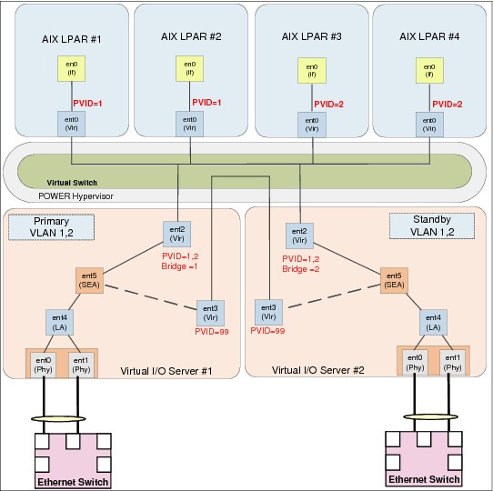
Figure 3-17 SEA failover configuration
|
Note: This is the simplest way to configure Shared Ethernet and is suitable in most cases. No special configuration is required on the client LPAR side.
|
3.7.2 SEA load sharing scenario
Figure 3-18 on page 85 demonstrates a feature known as SEA load sharing. This is in effect when there are multiple VLANs and the attribute ha_mode=sharing is enabled on the SEA on both VIOS. This option is available in VIOS 2.2.1.0 or later.
It is important to note that VLANs, not packets, are balanced between VIOS. This means that in a two VLAN scenario, one VLAN is active on one VIOS, while the other VLAN is active on the other VIOS. If one VLAN consists of the majority of network traffic, it is important to understand that the VIOS that this VLAN is active on will still be handling the majority of the network traffic.
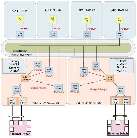
Figure 3-18 SEA load balancing scenario
|
Note: This method is suitable in cases where multiple VLANs are in use on a POWER System. This method is simple because no special configuration is required on the client LPAR side.
|
3.7.3 NIB with an SEA scenario
Figure 3-19 on page 86 shows a sample environment using Network Interface Backup (NIB). Typically, in this scenario all of the LPARs are using a single VLAN to the outside network, while internally they have two virtual Ethernet adapters, each with a different VLAN ID. This is used to send network packets to one of two separate SEA adapters, one per VIOS.
With NIB to load balance you could have half of the logical partitions sending traffic primarily to the first VIOS and in the event of a failover the second VIOS would be used, and the reverse is true for the other half of the logical partitions.
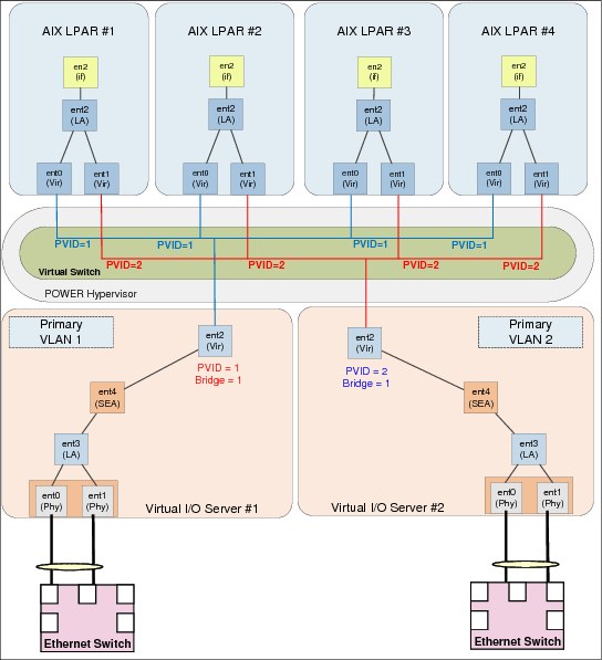
Figure 3-19 NIB scenario
|
Note: Special configuration is required on the client LPAR side. See 3.7.5, “Etherchannel configuration for NIB” on page 87 for details. VLAN tagging is also not supported in this configuration.
|
3.7.4 NIB with SEA, VLANs and multiple V-switches
Figure 3-20 on page 87 shows a sample environment using NIB with multiple virtual switches and VLAN tagging. In this scenario, there are two independent shared Ethernet adapters, each configured on a different virtual switch.
With NIB to load balance you could have half of the logical partitions sending traffic primarily to the first virtual switch and in the event of a failover the second virtual switch would be used, and the reverse for the other half of the logical partitions.

Figure 3-20 NIB with SEA, VLANs and multiple V-switches
|
Note: Special configuration is required on the client LPAR side. See 3.7.5, “Etherchannel configuration for NIB” on page 87 for details. This is the most complex method of configuring shared Ethernet.
|
3.7.5 Etherchannel configuration for NIB
In the event that NIB is used on the AIX LPAR using virtual Ethernet, there are some considerations to be made:
•There must be an IP address to ping that is outside the Power system. This ensures that the Etherchannel actually fails over.
•The Etherchannel will not fail back to the main channel automatically when the primary adapter recovers. It will only fail back when the backup adapter fails.
•When performing an installation via NIM, the IP address will be on one of the virtual adapters, and no Etherchannel device will exist. The adapters will need to be reconfigured in an Etherchannel configuration.
•It is suggested to balance the traffic per VIO server by having half of the VIO servers using one VIO server as the primary adapter, and the other half using the other VIO server as the backup adapter.
Example 3-26 demonstrates how to configure this feature with four AIX LPARs.
Example 3-26 Configuring NIB Etherchannel in AIX
root@aix1:/ #mkdev -c adapter -s pseudo -t ibm_ech -a adapter_names=ent0 -a backup_adapter=ent1 -a netaddr=192.168.100.1
ent2 Available
root@aix2:/ # mkdev -c adapter -s pseudo -t ibm_ech -a adapter_names=ent1 -a backup_adapter=ent0 -a netaddr=192.168.100.1
ent2 Available
root@aix3:/ # mkdev -c adapter -s pseudo -t ibm_ech -a adapter_names=ent0 -a backup_adapter=ent1 -a netaddr=192.168.100.1
ent2 Available
root@aix4:/ # mkdev -c adapter -s pseudo -t ibm_ech -a adapter_names=ent1 -a backup_adapter=ent0 -a netaddr=192.168.100.1
ent2 Available
3.7.6 VIO IP address assignment
For management purposes and the use of Live Partition Mobility (LPM), it is advised that each VIO server has an IP address assigned to it. There are multiple ways that an IP address can be configured:
•A dedicated adapter can be assigned to the VIO server for the management IP address.
•If you have a Host Ethernet Adapter in the Power System, an LHEA port can be used.
•The IP address can be put on the SEA.
•A separate virtual adapter can be assigned to the VIO server for the management IP address.
All of these methods are perfectly valid, and there are some implications and considerations when assigning the IP address.
If you are using LPM, it is suggested to have a separate adapter for LPM if possible. This ensures that the high network usage for LPM does not affect any traffic on the SEA. If this is not possible, ensure that the mover service partitions you are using for the LPM operation are not the VIO servers that are acting as primary in an SEA failover configuration.
From the testing we performed, there was no increase in latency and no decrease in throughput having the IP address on the SEA. This actually gave us two distinct advantages:
•We were able to use the entstat command on the SEA.
•We were able to use topas -E and collect more detailed SEA statistics with the -O option in the nmon recordings.
The only downside we found having the IP address for the VIO server on the SEA was that in the event of a failure on the SEA, the VIO server will not be reachable, so a terminal window from the HMC had to be used. However, having the VIO server acting as a client by having the IP address on a separate virtual adapter allowed us to take advantage of the SEA failover and maintain access to our VIO server.
There is no wrong answer for where to configure the IP address on the VIO server. However, depending on your environment there may be some advantages based on where you place the IP address.
3.7.7 Adapter choices
Choosing the number and type of Ethernet adapters for a shared network infrastructure is dependent on the server you have, and the workload you are placing on it.
There are a number of items that should be considered:
•What switch infrastructure exists on the network (1 Gb, 10 Gb)?
•How many gigabit or 10 gigabit adapters are required to supply the workload with sufficient bandwidth?
•Will dual VIOS be employed? If so, will each VIOS have sufficient resources to serve the entire workload in the event that one of the VIOS becomes unavailable?
•Will each VIOS require adapter redundancy? Where multiple adapters are placed in a link aggregation an increased throughput and ability to handle more packets will be gained.
•Is the workload sensitive to latency? If so, what is the latency of the network?
•What quantity and type of adapter slots are present in the server?
It is important to understand how your hardware will be configured to ensure that you will have sufficient resources for your workload. See Chapter 2, “Hardware implementation and LPAR planning” on page 7 for further details.
3.7.8 SEA conclusion
There are multiple ways to configure shared Ethernet on Power systems to provide both performance and redundancy for virtual networks. It is important to consider the method of shared Ethernet to implement, and the VLAN requirements for your environment.
It is also important to ensure that sufficient processor, memory and adapter bandwidth resources are available to your shared Ethernet implementation.
Table 3-10 provides a summary of the different shared Ethernet implementation methods, and when they could be used.
Table 3-10 SEA implementation method summary
|
Implementation Method
|
When to use
|
|
SEA failover
|
SEA failover is the typical way to implement shared Ethernet when you have an environment with one or more VLANs with dual VIO servers, and you do not want to have any special configuration on the client LPARs. This is the preferred method when you have a single VLAN. The presumed downside is that one VIO server handles all the traffic. However, you also know that if that VIO server fails, the other VIO server with identical configuration will handle all of the network traffic without degradation so this may not be a downside.
|
|
SEA failover with load sharing
|
SEA failover with load sharing is the preferred method when you have two or more VLANs. There is no special configuration required on the client LPAR side and VLANs are evenly balanced across the VIO servers. This balancing is based on the number of VLANs, not on the amount of traffic per VLAN. To force VLANs to use a specific SEA or VIO server, it may be required to use SEA failover with multiple SEA adapters with rotating bridge priorities between the VIO servers for each SEA and different VLANs assigned to each SEA. Where multiple SEAs are in use, it is strongly suggested to have each SEA on a different Vswitch.
|
|
NIB with no VLAN tagging
|
The VIO server configuration for this method is very straightforward because no control channel needs to be configured. However, there is special Ether channel configuration required on the client side. When balancing LPARs between the VIO servers, it is important that no VIO server is busy beyond 50% because a single VIO server may not have enough resources to support all the network traffic. VLAN tagging is not supported using this method.
|
|
NIB with Multiple Vswitches and VLAN tagging
|
This configuration method is more complicated, because multiple virtual switches need to be configured on the Power system, to enable VLAN tagging. There is also a requirement to have Ether channel configured on the client LPAR side. The same sizing requirement applies to ensure that the VIO servers are not busy beyond 50% to ensure that a single VIO server has the resources to support all of the network load.
|
|
Note: This section provides guidance on where different SEA configurations can be used. Ensure that the method you choose meets your networking requirements.
|
3.7.9 Measuring latency
Appreciating the latency in your network, be that between physical machines or adjacent LPARs, can be key in time-sensitive environments.
There are tools such as tcpdump available in AIX that provide the capability to measure network latency. It is important to profile latency when there is background traffic on the network, in addition to observing peak load. This will provide you with the perspective to understand whether there is a bottleneck or not.
Example 3-27 shows a sample shell script that can be run on an AIX system to measure the average latency between itself and a routable destination.
It is suggested to use this or something similar to measure the latency between LPARs on the same Power system, to measure latency across the hypervisor and to hosts outside of the physical system, and to measure latency to another system.
Example 3-27 netlatency.sh
#!/bin/ksh
usage () {
MESSAGE=$*
echo
echo "$MESSAGE"
echo
echo $0 -i INTERFACE -d dest_ip [ -c nb_packet ]
exit 3
}
tcpdump_latency () {
INTERFACE=$1
DEST_HOST=$2
COUNT=`echo "$3 * 2" | bc`
tcpdump -c$COUNT -tti $INTERFACE icmp and host $DEST_HOST 2>/dev/null | awk '
BEGIN { print "" }
/echo request/ { REQUEST=$1 ; SEQUENCE=$12 }
/echo reply/ && $12==SEQUENCE { COUNT=COUNT+1 ; REPLY=$1 ; LATENCY=(REPLY-REQUEST)*1000 ;
SUM=SUM+LATENCY ; print "Latency Packet " COUNT " : " LATENCY " ms"}
END { print ""; print "Average latency (RTT): " SUM/COUNT " ms" ; print""}
' &
}
COUNT=10
while getopts ":i:d:c:" opt
do
case $opt in
i) INTERFACE=${OPTARG} ;;
d) DEST_HOST=${OPTARG} ;;
c) COUNT=${OPTARG} ;;
?) usage USAGE
return 1
esac
done
##########################
# TEST Variable
[ -z "$INTERFACE" ] && usage "ERROR: specify INTERFACE"
[ -z "$DEST_HOST" ] && usage "ERROR: specify Host IP to ping"
############################
# MAIN
tcpdump_latency $INTERFACE $DEST_HOST $COUNT
sleep 1
OS=`uname`
case "$OS" in
AIX) ping -f -c $COUNT -o $INTERFACE $DEST_HOST > /dev/null ;;
Linux) ping -A -c$COUNT -I $INTERFACE $DEST_HOST > /dev/null ;;
?) echo "OS $OS not supported" ;exit 1
esac
exit 0
The script output in Example 3-28 shows the round trip latency of each packet and the average latency across the 20 packets. The script was executed with the following parameters:
•-i is the interface that we will be sending the traffic out of, in this case ent0.
•-d is the target host or device that we are testing latency between. In this case it is another AIX system with the hostname aix2.
•-c is the amount of packets we are going to send, in this case 20 packets.
Example 3-28 Latency test
root@aix1:/usr/local/bin # ./netlatency.sh -i en0 -d aix2 -c 20
Latency Packet 1 : 0.194788 ms
Latency Packet 2 : 0.0870228 ms
Latency Packet 3 : 0.0491142 ms
Latency Packet 4 : 0.043869 ms
Latency Packet 5 : 0.0450611 ms
Latency Packet 6 : 0.0619888 ms
Latency Packet 7 : 0.0431538 ms
Latency Packet 8 : 0.0360012 ms
Latency Packet 9 : 0.0281334 ms
Latency Packet 10 : 0.0369549 ms
Latency Packet 11 : 0.043869 ms
Latency Packet 12 : 0.0419617 ms
Latency Packet 13 : 0.0441074 ms
Latency Packet 14 : 0.0400543 ms
Latency Packet 15 : 0.0360012 ms
Latency Packet 16 : 0.0448227 ms
Latency Packet 17 : 0.0398159 ms
Latency Packet 18 : 0.0369549 ms
Latency Packet 19 : 0.0441074 ms
Latency Packet 20 : 0.0491142 ms
Average latency (RTT): 0.0523448 ms
The latency between AIX systems or between an AIX system and a device differs depending on network configuration and load on that network.
3.7.10 Tuning the hypervisor LAN
The Power hypervisor is used for network connectivity between client LPARs, as well as client LPAR connectivity to a VIOS for SEA access.
Figure 3-21 gives a simplified example of how a Power system may be configured, and we look closely at the connectivity on VLAN 100, which is simply used for LPAR communications.
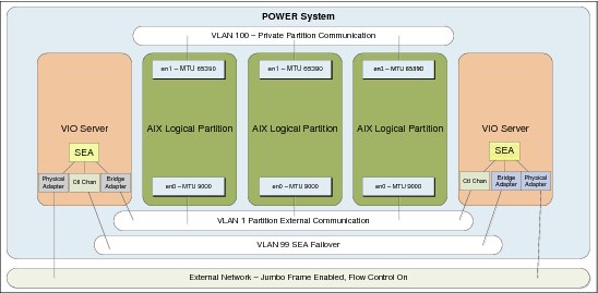
Figure 3-21 Sample configuration with separate VLAN for partition communication
The network may not be capable of accepting network packets with an MTU close to 64 k; so perhaps the VLAN for external communication on the Power system may have an MTU of 9000, and Jumbo Frames are enabled on the external network where we use a separate IP range on a different VLAN for partition communications. This can be particularly useful if one of the logical partitions on the Power system is a backup server LPAR, for example Tivoli Storage Manager (TSM) or a NIM server.
In Example 3-29 we can run a simple test using the netperf utility to perform a simple and repeatable bandwidth test between en0 in the aix1 LPAR and en0 on the aix2 LPAR in Figure 3-11 on page 65. The test duration will be 5 minutes.
Example 3-29 How to execute the netperf load
root@aix1:/ # netperf -H 192.168.100.12 -l 600
At this point in the example, all of the default AIX tunables are set. We can see in Figure 3-22 that the achieved throughput on this test was 202.7 megabytes per second.

Figure 3-22 Network throughput with default tunables and a single netperf stream
For the next test, we changed some tunables on the en0 interface utilizing the hypervisor network and observed the results of the test.
Table 3-11 describes some of the tunables that were considered prior to performing the test.
Table 3-11 AIX network tunables considered
|
Tunable
|
Description
|
Value
|
|
mtu size
|
Media Transmission Unit (MTU) size is the largest packet that AIX will send. Increasing the mtu size will typically increase performance for streaming workloads. The value 64390 is the maximum value minus VLAN overhead.
|
65390 (for large throughput)
|
|
flow control
|
Flow control is a TCP technique which will match the transmission rate of the sender with the transmission rate of the receiver. This is enabled by default in AIX.
|
on
|
|
large send
|
The TCP large send offload option enables AIX to build a TCP message up to 64 KB in size for transmission.
|
on
|
|
large receive
|
The TCP large receive offload option enables AIX to aggregate multiple received packets into a larger buffer reducing the amount of packets to process.
|
on
|
|
rfc1323
|
This tunable, when set to 1, enables TCP window scaling when both ends of a TCP connection have rfc1323 enabled.
|
1
|
|
tcp send or receive space
|
These values specify how much data can be buffered when sending or receiving data. For most workloads the default of 16384 is sufficient. However, in high latency situations these values may need to be increased.
|
16384 is the default, increasing to 65536 may provide some increased throughput.
|
|
checksum offload
|
This option allows the network adapter to compute the TCP checksum rather than the AIX system performing the computation. This is only valid for physical adapters.
|
yes
|
|
dcbflush_local
|
Data Cache Block Flush (dcbflush) is an attribute for a virtual Ethernet adapter that allows the virtual Ethernet device driver to flush the processor’s data cache of any data after it has been received.
|
yes
|
These tunables are discussed in more detail in the AIX 7.1 Information Center at:
|
Note: It is important to try tuning each of these parameters individually and measuring the results. Your results may vary from the tests performed in this book. It is also expected that changes occur in processor and memory utilization as a result of modifying these tunables.
|
Example 3-30 demonstrates the tuning changes we made during the test. These changes included:
•Increasing the MTU size on both AIX LPARs from 1500 to 64390.
•Enabling largesend using the mtu_bypass option.
•Enabling Data Cache Block Flush with the dcbflush_local option. Note that the interface had to be down for this change to be applied.
•Enabling rfc1323 to take effect and to be persistent across reboots.
Example 3-30 Apply tunables to AIX logical partitions
root@aix1:/ # chdev -l en0 -a mtu=65390
en0 changed
root@aix1:/ # chdev -l en0 -a mtu_bypass=on
en0 changed
root@aix1:/ # chdev -l en0 -a state=down
en0 changed
root@aix1:/ # chdev -l en0 -a state=detach
en0 changed
root@aix1:/ # chdev -l ent0 -a dcbflush_local=yes
ent0 changed
root@aix1:/ # chdev -l en0 -a state=up
en0 changed
root@aix1:/ # no -p -o rfc1323=1
Setting rfc1323 to 1
Setting rfc1323 to 1 in nextboot file
Change to tunable rfc1323, will only be effective for future connections
root@aix1:/ #
root@aix2:/ # chdev -l en0 -a mtu=65390
en0 changed
root@aix2:/ # chdev -l en0 -a mtu_bypass=on
en0 changed
root@aix2:/ # chdev -l en0 -a state=down
en0 changed
root@aix2:/ # chdev -l en0 -a state=detach
en0 changed
root@aix2:/ # chdev -l ent0 -a dcbflush_local=yes
ent0 changed
root@aix2:/ # chdev -l en0 -a state=up
en0 changed
root@aix2:/ # no -p -o rfc1323=1
Setting rfc1323 to 1
Setting rfc1323 to 1 in nextboot file
Change to tunable rfc1323, will only be effective for future connections
root@aix2:/ #
|
Note: Example 3-30 on page 94 requires that the en0 interface is down for some of the settings to be applied.
|
If the mtu_bypass option is not available on your adapter, run the tunable as follows instead; however, this change is not persistent across reboots. You need to add this to /etc/rc.net to ensure that largesend is enabled after a reboot (Example 3-31).
Example 3-31 Enable largesend with ifconfig
root@aix1:/ # ifconfig en0 largesend
root@aix1:/ #
root@aix2:/ # ifconfig en0 largesend
root@aix2:/ #
Figure 3-23 shows the next netperf test performed in exactly the same way as Example 3-29 on page 93. It is noticeable that this test delivered over a 7x improvement in throughput.

Figure 3-23 Network throughput with modified tunables and a single netperf stream
Figure 3-24 shows additional netperf load using additional streams to deliver increased throughput, demonstrating that the capable throughput is dependant on how network intensive the workload is.

Figure 3-24 Network throughput with modified tunables again, but with additional netperf load
3.7.11 Dealing with dropped packets on the hypervisor network
When load on a virtual Ethernet adapter is heavy, there is a situation that will occur when two items become an issue:
•Latency increased across the hypervisor network between logical partitions. “Etherchannel configuration for NIB” on page 87 describes network latency. It is important to monitor the latency of the network.
•The virtual Ethernet adapter’s receive buffers are exhausted and packets will be retransmitted and thoughput will decrease. This is shown in Example 3-32 where the aix1 LPAR is experiencing dropped packets.
– Packets Dropped is the total amount of packets that could not be received by the aix1 LPAR.
– No Resource Errors is the total number of times that the aix1 LPAR was unable to receive any more packets due to lack of buffer resources.
– Hypervisor Receive Failures is the total number of packets the hypervisor could not deliver to because the receive queue was full.
– Hypervisor Send Failures is the total number of times that a packet could not be sent due to a buffer shortage.
Example 3-32 The netstat -v output demonstrating dropped packets
root@aix1:/ # netstat -v ent0
-------------------------------------------------------------
ETHERNET STATISTICS (ent0) :
Device Type: Virtual I/O Ethernet Adapter (l-lan)
Hardware Address: 52:e8:7f:a2:19:0a
Elapsed Time: 0 days 0 hours 35 minutes 48 seconds
Transmit Statistics: Receive Statistics:
-------------------- -------------------
Packets: 76773314 Packets: 39046671
Bytes: 4693582873534 Bytes: 45035198216
Interrupts: 0 Interrupts: 1449593
Transmit Errors: 0 Receive Errors: 0
Packets Dropped: 0 Packets Dropped: 8184
Bad Packets: 0
Max Packets on S/W Transmit Queue: 0
S/W Transmit Queue Overflow: 0
Current S/W+H/W Transmit Queue Length: 0
Broadcast Packets: 14 Broadcast Packets: 4474
Multicast Packets: 8 Multicast Packets: 260
No Carrier Sense: 0 CRC Errors: 0
DMA Underrun: 0 DMA Overrun: 0
Lost CTS Errors: 0 Alignment Errors: 0
Max Collision Errors: 0 No Resource Errors: 8184
Late Collision Errors: 0 Receive Collision Errors: 0
Deferred: 0 Packet Too Short Errors: 0
SQE Test: 0 Packet Too Long Errors: 0
Timeout Errors: 0 Packets Discarded by Adapter: 0
Single Collision Count: 0 Receiver Start Count: 0
Multiple Collision Count: 0
Current HW Transmit Queue Length: 0
General Statistics:
-------------------
No mbuf Errors: 0
Adapter Reset Count: 0
Adapter Data Rate: 20000
Driver Flags: Up Broadcast Running
Simplex 64BitSupport ChecksumOffload
DataRateSet
Virtual I/O Ethernet Adapter (l-lan) Specific Statistics:
---------------------------------------------------------
RQ Length: 4481
Trunk Adapter: False
Filter MCast Mode: False
Filters: 255
Enabled: 2 Queued: 0 Overflow: 0
LAN State: Operational
Hypervisor Send Failures: 2090
Receiver Failures: 2090
Send Errors: 0
Hypervisor Receive Failures: 8184
Invalid VLAN ID Packets: 0
ILLAN Attributes: 0000000000003002 [0000000000003002]
Port VLAN ID: 1
VLAN Tag IDs: None
Switch ID: ETHERNET0
Hypervisor Information
Virtual Memory
Total (KB) 79
I/O Memory
VRM Minimum (KB) 100
VRM Desired (KB) 100
DMA Max Min (KB) 128
Transmit Information
Transmit Buffers
Buffer Size 65536
Buffers 32
History
No Buffers 0
Virtual Memory
Total (KB) 2048
I/O Memory
VRM Minimum (KB) 2176
VRM Desired (KB) 16384
DMA Max Min (KB) 16384
Receive Information
Receive Buffers
Buffer Type Tiny Small Medium Large Huge
Min Buffers 512 512 128 24 24
Max Buffers 2048 2048 256 64 64
Allocated 512 512 156 24 64
Registered 511 512 127 24 18
History
Max Allocated 512 512 165 24 64
Lowest Registered 511 510 123 22 12
Virtual Memory
Minimum (KB) 256 1024 2048 768 1536
Maximum (KB) 1024 4096 4096 2048 4096
I/O Memory
VRM Minimum (KB) 4096 4096 2560 864 1632
VRM Desired (KB) 16384 16384 5120 2304 4352
DMA Max Min (KB) 16384 16384 8192 4096 8192
I/O Memory Information
Total VRM Minimum (KB) 15524
Total VRM Desired (KB) 61028
Total DMA Max Min (KB) 69760
root@aix1:/ #
Under Receive Information in the netstat -v output in Example 3-32 on page 96, the type and number of buffers are listed. If at any point the Max Allocated under history reaches the max Buffers in the netstat -v output, it may be required to increase the buffer size to help overcome this issue.
Our max_buf_huge was exhausted due to the nature of the netperf streaming workload. The buffers which may require tuning are very dependant on workload and it is advisable to tune these only under the guidance of IBM support. Depending on the packet size and number of packets, different buffers may need to be increased. In our case it was large streaming packets, so only huge buffers needed to be increased.
Example 3-33 demonstrates how to increase the huge buffers for the ent0 interface. The en0 interface will need to be brought down for this change to take effect.
Example 3-33 How to increase the virtual Ethernet huge buffers
root@aix1:/ # chdev -l en0 -a state=down
en0 changed
root@aix1:/ # chdev -l en0 -a state=detach
en0 changed
root@aix1:/ # chdev -l ent0 -a min_buf_huge=64 -a max_buf_huge=128
ent0 changed
root@aix1:/ # chdev -l en0 -a state=up
en0 changed
root@aix1:/ #
|
Note: We suggest to review the processor utilization before making any changes to the virtual Ethernet buffer tuning. Buffers should only be tuned if the allocated buffers reaches the maximum buffers. If in doubt, consult with IBM support.
|
3.7.12 Tunables
Typically, VIOS are deployed in pairs, and when Ethernet sharing is in use each VIOS has a physical adapter that acts as a bridge for client LPARs to access the outside network.
Physical tunables
It is important to ensure that the physical resources that the shared Ethernet adapter is built on top of are configured for optimal performance. 4.5.1, “Network tuning on 10 G-E” on page 186 describes in detail how to configure physical Ethernet adapters for optimal performance.
EtherChannel tunables
When creating a Link Aggregation that a SEA is built on top of, it is important to consider the options available when configuring the EtherChannel device.
There are a number of options available when configuring aggregation; we suggest to consider the following:
•mode - This is the EtherChannel mode of operation. A suggested value is 8023ad.
•use_jumbo_frame - This enables Gigabit Ethernet Jumbo Frames.
•hash_mode - This determines how the outgoing adapter is chosen. A suggested value is src_dst_port.
Example 3-34 demonstrates how to create a link aggregation using these options.
Example 3-34 Creation of the link aggregation
$ mkvdev -lnagg ent1,ent2 -attr mode=8023ad hash_mode=src_dst_port use_jumbo_frame=yes
ent5 Available
en5
et5
$
SEA tunables
When creating an SEA it is important to consider the options available to improve performance on the defined device.
Options that should be considered are:
•jumbo_frames - This enables gigabit Ethernet jumbo frames.
•large_receive - This enables TCP segment aggregation,
•largesend - This enables hardware transmit TCP resegmentation.
Example 3-35 demonstrates how to create a shared Ethernet adapter on top of the ent5 EtherChannel device using ent3 as the bridge adapter and ent4 as the control channel adapter.
Example 3-35 Creation of the shared Ethernet adapter
$ mkvdev -sea ent5 -vadapter ent3 -default ent3 -defaultid 1 -attr ha_mode=auto ctl_chan=ent4 jumbo_frames=yes large_receive=yes largesend=1
ent6 Available
en6
et6
$
Monitoring and accounting
Accounting can be enabled for an SEA that at the time of writing is not enabled by default. It is suggested that this option be enabled to allow use of seastat to report SEA-related statistics.
Example 3-36 demonstrates how to enable SEA accounting.
Example 3-36 Enabling SEA accounting
$ lsdev -type adapter |grep "Shared Ethernet Adapter"
ent6 Available Shared Ethernet Adapter
$ chdev -dev ent6 -attr accounting=enabled
ent6 changed
$ lsdev -dev ent6 -attr |grep accounting
accounting enabled Enable per-client accounting of network statistics True
$
|
Any tunables that have been applied to the SEA on the VIOS, the adapter or devices it is defined onto, must match the switch configuration. This includes but is not limited to:
•EtherChannel mode; for example, 8023.ad
•Jumbo frames
•Flow control
|
3.8 PowerVM virtualization stack configuration with 10 Gbit
The PowerVM virtualization stack (Figure 3-25 on page 101) consists of the Virtual I/O Server with Shared Ethernet Adapter (SEA) backed by physical Ethernet adapters with or without link aggregation (Etherchannels), virtual Ethernet trunk adapters, and AIX or Linux or IBM i partitions with virtual Ethernet adapters.
Between the virtual Ethernet adapters are the hypervisor virtual switches.
Beyond the physical Ethernet adapters are the actual physical network, with switches, routers, and firewalls, all of which impact network throughput, latency and round trip times.

Figure 3-25 PowerVM virtualization stack overview
In some network environments, network and virtualization stacks, and protocol endpoint devices, other settings might apply.
|
Note: Apart from LRO, the configuration is also applicable for 1 Gbit.
|
Gigabit Ethernet and VIOS SEA considerations:
1. For optimum performance, ensure adapter placement according to Adapter Placement Guide, and size VIOS profile with sufficient memory and processing capacity to fit the expected workload, such as:
– No more than one 10 Gigabit Ethernet adapter per I/O chip.
– No more than one 10 Gigabit Ethernet port per two processors in a system.
– If one 10 Gigabit Ethernet port is present per two processors in a system, no other 10 Gb or 1 Gb ports should be used.
2. Each switch port
– Verify that flow control is enabled.
3. On each physical adapter port in the VIOS (ent).chksum_offload enabled (default)
– flow_ctrl enabled (default)
– large_send enabled (preferred)
– large_receive enabled (preferred)
– jumbo_frames enabled (optional)
– Verify Adapter Data Rate for each physical adapter (entstat -d/netstat -v)
4. On the Link Aggregation in the VIOS (ent)
– Load Balance mode (allow the second VIOS to act as backup)
– hash_mode to src_dst_port (preferred)
– mode to 8023ad (preferred)
– use_jumbo_frame enabled (optional)
– Monitor each physical adapter port with entstat command to determine the selected hash_mode effectiveness in spreading the outgoing network load over the link aggregated adapters
5. On the SEA in the VIOS (ent)
– largesend enabled (preferred)
– jumbo_frames enabled (optional)
– netaddr set for primary VIOS (preferred for SEA w/failover)
• Use base VLAN (tag 0) to ping external network address (beyond local switch).
• Do not use switch or router virtual IP address to ping (if its response time might fluctuate).
– Consider disabling SEA thread mode for SEA only VIOS.
– Consider implementing VLAN load sharing.
• http://pic.dhe.ibm.com/infocenter/powersys/v3r1m5/index.jsp?topic=/p7hb1/iphb1_vios_scenario_sea_load_sharing.htm
• http://www-01.ibm.com/support/docview.wss?uid=isg3T7000527
6. On the virtual Ethernet adapter in the VIOS (ent)
– chksum_offload enabled (default)
– Consider enabling dcbflush_local
– In high load conditions, the virtual Ethernet buffer pool management of adding and reducing the buffer pools on demand can introduce latency of handling packets (and can result in drops of packets, “Hypervisor Receive Failures”).
• Setting the “Min Buffers” to the same value as “Max Buffers” allowed will eliminate the action of adding and reducing the buffer pools on demand. However, this will use more pinned memory.
• For VIOS in high end servers, you might also have to increase the max value to its maximum allowed, and then increase the min value accordingly. Check the maximum value with the lsattr command, such as: lsattr -Rl ent# -a max_buf_small
• Max buffer sizes: Tiny (4096), Small (4096), Medium (2048), Large (256), Huge (128)
7. On the virtual Ethernet adapter in the virtual client/partition (ent)
– chksum_offload enabled (default)
• Monitoring utilization with enstat -d or netstat -v and if “Max Allocated” is higher than “Min Buffers”, increase to higher value than “Max Allocated” or to “Max Buffers”, for example: Increase the "Min Buffers“ to be greater than "Max Allocated" by increasing it up to the next multiple of 256 for "Tiny" and "Small" buffers, by the next multiple of 128 for "Medium" buffers, by the next multiple of 16 for "Large“ buffers, and by the next multiple of 8 for "Huge" buffers.
8. On the virtual network interface in the virtual client/partition (en)
– mtu_bypass enabled
• Is the largesend attribute for virtual Ethernet (AIX 6.1 TL7 SP1 or AIX7.1 SP1)
• If not available, set with the ifconfig command after each partition boot in /etc/rc.net or equiv by init, for example: ifconfig enX largesend
– Use the device driver built-in interface specific network options (ISNO)
• ISNO is enabled by default (the no tunable use_isno).
• Device drivers have default settings, leave the default values intact.
• Check current settings with the ifconfig command.
• Change with the chdev command.
• Can override with the ifconfig command or setsockopt() options.
– Set mtu to 9000 if using jumbo frames (network support required)
• Default mtu is 1500 (Maximum Transmission Unit/IP)
• Default mss is 1460 (Maximum segment Size/TCP) with RFC1323 disabled
• Default mss is 1448 (Maximum segment Size/TCP) with RFC1323 enabled
– Consider enabling network interface thread mode (dog thread)
• Set with the ifconfig command, for example: ifconfig enX thread
• Check utilization with the netstat command: netstat -s| grep hread
• For partitions with dozens of VPs, review the no tunable ndogthreads
• http://pic.dhe.ibm.com/infocenter/aix/v7r1/index.jsp?topic=/com.ibm.aix.prftungd/doc/prftungd/enable_thread_usage_lan_adapters.htm
A note on monitoring adapter port transmit statistics to determine how the actual workload spreads the network traffic over link aggregated (Etherchanneled) adapter ports.
Use the entstat command (or netstat -v) and summarize, as in Table 3-12. In this case we deploy an adapter port link aggregation in 8023ad mode using default hash_mode.
The lsattr command:
adapter_names ent0,ent1,ent4,ent6 EtherChannel Adapters
hash_mode default Determines how outgoing adapter is chosen
mode 8023ad EtherChannel mode of operation
The statistics in this case show that the majority of the outgoing (transmit) packets go out over ent6, and approximately 1/3 of the total packets go out over ent4, with ent0 and ent1 practically unused for outgoing traffic (the receive statistics are more related to load balancing from the network side, and switch MAC tables and trees).
Table 3-12 Etherchannel/Link Aggregation statistics with hash_mode default
|
Device
|
Transmit packets
|
% of total
|
Receive packets
|
% of total
|
|
ent0
|
811028335
|
3%
|
1239805118
|
12%
|
|
ent1
|
1127872165
|
4%
|
2184361773
|
21%
|
|
ent4
|
8604105240
|
28%
|
2203568387
|
21%
|
|
ent6
|
19992956659
|
65%
|
4671940746
|
45%
|
|
Total
|
29408090234
|
100%
|
8115314251
|
100%
|
3.9 AIX Workload Partition implications, performance and suggestions
Workload Partitions (WPARs) were introduced with AIX 6.1 in 2007. A WPAR is a software implementation of partitioning provided just by the operating system. The WPAR components have been regularly enhanced with subsequent AIX releases, including IPv6 and NPIV support. AIX 7.1 also introduced the notable addition of Versioned WPARs. This feature allows both AIX 5.2 and 5.3 to be hosted in a WPAR.
3.9.1 Consolidation scenario
This first scenario uses WPARs as a consolidation vehicle to collapse three LPARs into one larger LPAR. We demonstrate the sequence to migrate from LPAR to WPAR and discuss our observations about sizing and performance that should be considered for such implementations.
Our scenario begins with three AIX 7.1 TL02 LPARs hosted on a Power 750 server. Figure 3-26 provides a high-level view of this scenario.

Figure 3-26 LPAR to WPAR scenario
The three LPARs were indentical in size. Table 3-13 details the LPAR resource configuration. The LPARs were generically defined for the test case—they were not sized based on their hosted workload footprint.
Table 3-13 LPAR configuration of consolidation candidates
|
CPU
|
RAM
|
Storage
|
|
4 VPs, EC 1.0, uncapped
|
8 GB (dedicated)
|
60 GB (via vSCSI)
|
Each LPAR hosted a deployment of our WebSphere Message Broker sample application. However, the application was configured differently on each LPAR to give a footprint; the sample application was configured to run with one application thread on LPAR1, two on LPAR2, and eight on LPAR4. So while the hosted application was the same, we were consolidating three different footprints.
A fourth LPAR was created with the same allocation of four VPs and 8 GB, but with additional storage. A secondary volume group was created of 120 GB to host the WPARs. This separation from rootvg was implemented to avoid any unnecessary contention or background noise.
For each LPAR, we ran the sample application for 10 minutes to obtain a baseline TPS. The applications were quiesced and a clean mksysb backup taken of each LPAR.
After transferring the mksysb files to the fourth LPAR, we used a new feature of the mkwpar command introduced with AIX 7.1 TL02. The additional functionality introduces a variant of a System WPAR called a System Copy WPAR. It allows a System WPAR to be created from a mksysb; so the feature is similar in operation to the creation of a Versioned WPAR.
|
Note: For reference the mksysb can be as old as AIX 4.3.3, but part of the deployment process requires the created WPAR to be synchronized to the level of the hosting Global system before it can be started.
|
Example 3-37 shows the mkwpar command used to create one of the System Copy WPARs.
Example 3-37 mkwpar command
# mkwpar -n WPAR1 -g wparvg -h p750s2aix2wp4 -N interface=en0 address=192.168.100.100 netmask=255.255.255.0 -A -s -t -B /export/mksysb_LPAR1
Parameters of interest are -g, which overrides the hosting volume group (the default is rootvg); -t, which informs the command to copy rootvg from a system backup specified by the subsequent -B flag.
The process was repeated to create a second and third WPAR. No resource controls were implemented on any of the WPARs. Example 3-38 shows the output from the lswpar command after all three were created.
Example 3-38 lswpar command
# lswpar
Name State Type Hostname Directory RootVG WPAR
-------------------------------------------------------------
WPAR1 A S p750s2aix2wp1 /wpars/WPAR1 no
WPAR2 A S p750s2aix2wp2 /wpars/WPAR2 no
WPAR3 A S p750s2aix2wp3 /wpars/WPAR3 no
The time required to create a WPAR from an mksysb will naturally vary depending on the size of your mksysb. In our case it took around 5 minutes per WPAR.
Having successfully created our WPARs, we verified that all required file systems and configurations were preserved from the mksysb. mkwpar had successfully deployed a WPAR from the given mksysb; file systems were intact and the Message Broker application restarted clean in all three cases.
Next we repeated the 10-minute WebSphere Message Broker workload, running individually in each WPAR in parallel; that is, all three WPARs were active and running their own workload at the same time. This gave an initial comparison of how the workloads performed compared to running in isolation on an LPAR. But it also demonstrated how the three workloads tolerated the initial sizing of the hosting LPAR.
Because this scenario is based around consolidation, for simplicity we will normalize the performance of the three WPARs as a percentage of the TPS obtained by the baseline LPARs. For example, with our initial configuration of 4VP, the three WPARs in parallel delivered approximately 78% of the combined baseline TPS. First impressions may suggest this is a worrying result; however, remember that the Global LPAR has a third of the processor allocation compared to the original LPARs. The three LPARs combined had a total of 12 VPs, compared to the hosting LPAR, which had four. In context, 78% is actually quite encouraging.
We continued by amending the processor allocation and rerunning the workloads to profile the change in TPS. The LPAR was increased from 4VP in increments up to 12VP. We also tried a configuration of dedicated processor allocation as a comparison. Figure 3-27 illustrates the %TPS delivered by the five different configurations.

Figure 3-27 Global LPAR TPS
So for our scenario, when considering the combined workloads as a whole, 8VP proved to be the better configuration. Interestingly, the dedicated processor configuration was less efficient than a shared-processor LPAR of the same allocated size.
Illustrating the usage from another angle, Table 3-14 lists the average processor consumption during the 10-minute duration baseline on the original LPARs.
Table 3-14 LPAR CPU consumption
|
LPAR
|
LPAR1
|
LPAR2
|
LPAR3
|
|
Processor consumption
|
1.03
|
2.06
|
3.80
|
Almost 7.0 processor units were required for the three LPARs. Compare that to the results obtained for the 4VP configuration that consumed only 3.95 units. Another viewpoint is that approximately 57% of the processor resource produced 66% of the original throughput. It is important to consider the difference in consumed resource, compared to the combined throughput. The sustained consumption from the other configurations is listed in Table 3-15 on page 107.
Table 3-15 Global LPAR processor consumption
|
Virtual processor assignment
|
4VP
|
6VP
|
8VP
|
12VP
|
|
Processor consumption
|
3.95
|
5.50
|
7.60
|
9.30
|
The figures show that as the VPs increased, the utilization ultimately peaked and then dropped. The results in Table 3-15 conclude that 8VP was the better configuration for our tests, because 8VPs provided the best TPS of the tested configurations and the processor consumption was only marginally higher than the sum of the original LPARs. This suggested that the overhead for the Global LPAR was actually quite small. However, we were still concerned about the differences in observed TPS.
One thought was that Global LPAR hosting the WPARs was part of the cause. To rule this out we ran the workloads independently, with the Global LPAR in the 8VP configuration, with only one given WPAR active at once. Table 3-16 shows the percentage of throughput compared to the associated original LPAR; in each case more than 100% was achieved.
Table 3-16 Individual WPAR performance compared to individual LPAR
|
Application threads
|
Percentage
|
|
1
|
119%
|
|
2
|
116%
|
|
8
|
150%
|
Completing the analysis of this scenario, we compared the overhead of the original three LPARs and the hosting Global LPAR for the amount of hypervisor calls. We expected that a single LPAR should be less of an overhead than three; however, it was unclear from available documentation whether the use of WPARs would significantly increase calls to the hypervisor. We reran our 10-minute workloads and used lparstat to record the hypervisor call activity over the duration and provide a per-second average.
For our scenario we found the comparison between the sum of the LPARs and the Global LPAR quite surprising. The Global LPAR used 42% fewer hypervisor calls (per second) compared to the sum of the three LPARs. This is because the LPAR was containing some of the hosting overhead normally placed onto the hypervisor. It is important to appreciate the benefit of reducing unnessary load on the hypervisor; this frees up processor cycles for other uses such as shared processor and memory management, Virtual Ethernet operations, and dynamic LPAR overheads.
The difference in results between the original LPARs, compared to the various configurations of WPARs results from the contention of the primary SMT threads on each VP. Running isolation on an LPAR, there is no competition for the workload. Even when the host LPAR had the same resources as the combined three LPARs, there is enough contention between the workloads to result in the degradation of the smaller workloads. The larger workload actually benefits from there being more VPs to distribute work across.
When a workload test was in progress, we used nmon to observe the process usage across a given allocation. This allowed us to appreciate how the footprint of the whole Global LPAR changed as the resources were increased; nmon also allowed us to track the distribution and usage of SMT threads across the LPAR.
To complete the investigations on our consolidation scenario, we looked at memory. We used amepat to profile memory usage from the Global LPAR (configured with 8VP) and reconfigured the LPAR based on its recommendation. We subsequently reran the workloads and reprofiled with amepat two further times to gain a stable recommendation. The stable recommendation reconfigured the LPAR from 8 GB down to 4 GB. However, we did record approximately 10% TPS reduction of the workloads.
We started with three LPARs, with a total of 12 VP, 24 GB RAM and 180 GB of disk. We demonstrated that with our given workload, the smaller cases suffered slightly due to scheduling competition between the WPARs, whereas the larger workload benefitted slightly from the implementation. The final LPAR configuration had 8 VP, 4 GB RAM and 180 GB of disk. Of the 120 GB allocated in the secondary volume group, only 82 GB were used to host the three WPARs. The final configuration had 75% of the original processor, 17% of the RAM and 45% of the storage. With that greatly reduced footprint, the one LPAR provided 79% of the original throughput. So throughput has been the trade-off for an increase in resource efficiency.
3.9.2 WPAR storage
There are a number of ways to present disk storage to an AIX Workload Partition (WPAR). Depending on the use case, the methods of disk presentation may be different, and have differing performance characteristics.
There are two types of WPARs described here:
•A rootvg WPAR - This is a WPAR built on an hdisk device that is dedicated to the WPAR. The WPAR has its own exclusive rootvg on this disk device. It is not possible to have a versioned WPAR built on a rootvg WPAR.
•A system WPAR - This is a WPAR that has its own root volume group which is built on file systems and logical volumes created inside the global environment. Where versioned WPARs are used, they must be of a system WPAR type.
This subsection discusses some different methods of storage presentation grouped into two areas: Presenting block storage (devices) and file storage (providing access to a file system).
|
Note: For further information related to WPARs, refer to Exploiting IBM AIX Workload Partitions, SG24-7955.
|
Block
Block storage presentation in this section refers to presenting LUNs, seen as hdisk devices to an AIX WPAR.
There are two methods to achieve this outcome:
•Taking a LUN (hdisk device) from the AIX global instance and presenting it to a WPAR using the chwpar command. This can be performed on a system or rootvg WPAR.
•Presenting one or more physical or NPIV fiber channel adapters from the global AIX instance to the WPAR, again using the chwpar command. It is not possible to present adapters to a rootvg or versioned WPAR. WPAR mobility is also not possible when mapping adapters to a WPAR.
Figure 3-28 on page 109 illustrates the different methods of presenting disks to a WPAR.
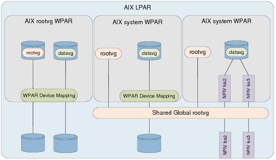
Figure 3-28 WPAR block storage access methods
When mapping a LUN (hdisk) device to a WPAR, the queue_depth and max_transfer settings can be applied as discussed in 4.3.2, “Disk device tuning” on page 143 with the exception of the algorithm attribute, which only supports fail_over.
Example 3-39 demonstrates how to take the device hdisk6 from the AIX global instance, and present it to a WPAR. Once the disk is exported, it is defined in the global AIX and available in the WPAR.
Example 3-39 WPAR disk device mapping
root@aix1global:/ # lsdev -Cc disk |grep hdisk6
hdisk6 Available 02-T1-01 MPIO FC 2145
root@aix1global:/ # chwpar -D devname=hdisk6 aix71wp
root@aix1global:/ # lsdev -Cc disk |grep hdisk6
hdisk6 Defined 02-T1-01 MPIO FC 2145
root@aix1global:/ # lswpar -D aix71wp
Name Device Name Type Virtual Device RootVG Status
-------------------------------------------------------------------
aix71wp hdisk6 disk no EXPORTED
aix71wp /dev/null pseudo EXPORTED
aix71wp /dev/tty pseudo EXPORTED
aix71wp /dev/console pseudo EXPORTED
aix71wp /dev/zero pseudo EXPORTED
aix71wp /dev/clone pseudo EXPORTED
aix71wp /dev/sad clone EXPORTED
aix71wp /dev/xti/tcp clone EXPORTED
aix71wp /dev/xti/tcp6 clone EXPORTED
aix71wp /dev/xti/udp clone EXPORTED
aix71wp /dev/xti/udp6 clone EXPORTED
aix71wp /dev/xti/unixdg clone EXPORTED
aix71wp /dev/xti/unixst clone EXPORTED
aix71wp /dev/error pseudo EXPORTED
aix71wp /dev/errorctl pseudo EXPORTED
aix71wp /dev/audit pseudo EXPORTED
aix71wp /dev/nvram pseudo EXPORTED
aix71wp /dev/kmem pseudo EXPORTED
root@aix1global:/ # clogin aix71wp
*******************************************************************************
* *
* *
* Welcome to AIX Version 7.1! *
* *
* *
* Please see the README file in /usr/lpp/bos for information pertinent to *
* this release of the AIX Operating System. *
* *
* *
*******************************************************************************
Last unsuccessful login: Mon Oct 8 12:39:04 CDT 2012 on ssh from 172.16.253.14
Last login: Fri Oct 12 14:18:58 CDT 2012 on /dev/Global from aix1global
root@aix71wp:/ # lsdev -Cc disk
root@aix71wp:/ # cfgmgr
root@aix71wp:/ # lsdev -Cc disk
hdisk0 Available 02-T1-01 MPIO FC 2145
root@aix71wp:/ #
The other method of presenting block devices to AIX is to present physical adapters to the partition. These could also be NPIV. The method is exactly the same. It is important that any SAN zoning is completed prior to presenting the adapters, and device attributes discussed in 4.3.5, “Adapter tuning” on page 150 are configured correctly in the global AIX before the device is exported. These settings are passed through to the WPAR, and can be changed inside the WPAR if required after the device is presented.
Example 3-40 demonstrates how to present two NPIV fiber channel adapters (fcs2 and fcs3) to the WPAR. When the mapping is performed, the fcs devices change to a defined state in the global AIX instance, and become available in the WPAR. Any child devices such as a LUN (hdisk device) are available on the WPAR.
Example 3-40 WPAR NPIV mapping
root@aix1global:/ # chwpar -D devname=fcs2 aix71wp
fcs2 Available
fscsi2 Available
sfwcomm2 Defined
fscsi2 Defined
line = 0
root@aix1global:/ # chwpar -D devname=fcs3 aix71wp
fcs3 Available
fscsi3 Available
sfwcomm3 Defined
fscsi3 Defined
line = 0
root@aix1global:/ # lswpar -D aix71wp
Name Device Name Type Virtual Device RootVG Status
--------------------------------------------------------------------
aix71wp fcs3 adapter EXPORTED
aix71wp fcs2 adapter EXPORTED
aix71wp /dev/null pseudo EXPORTED
aix71wp /dev/tty pseudo EXPORTED
aix71wp /dev/console pseudo EXPORTED
aix71wp /dev/zero pseudo EXPORTED
aix71wp /dev/clone pseudo EXPORTED
aix71wp /dev/sad clone EXPORTED
aix71wp /dev/xti/tcp clone EXPORTED
aix71wp /dev/xti/tcp6 clone EXPORTED
aix71wp /dev/xti/udp clone EXPORTED
aix71wp /dev/xti/udp6 clone EXPORTED
aix71wp /dev/xti/unixdg clone EXPORTED
aix71wp /dev/xti/unixst clone EXPORTED
aix71wp /dev/error pseudo EXPORTED
aix71wp /dev/errorctl pseudo EXPORTED
aix71wp /dev/audit pseudo EXPORTED
aix71wp /dev/nvram pseudo EXPORTED
aix71wp /dev/kmem pseudo EXPORTED
root@aix1global:/ # clogin aix71wp
*******************************************************************************
* *
* *
* Welcome to AIX Version 7.1! *
* *
* *
* Please see the README file in /usr/lpp/bos for information pertinent to *
* this release of the AIX Operating System. *
* *
* *
*******************************************************************************
Last unsuccessful login: Mon Oct 8 12:39:04 CDT 2012 on ssh from 172.16.253.14
Last login: Fri Oct 12 14:22:03 CDT 2012 on /dev/Global from p750s02aix1
root@aix71wp:/ # lsdev -Cc disk
root@aix71wp:/ # cfgmgr
root@aix71wp:/ # lsdev -Cc disk
hdisk0 Available 03-T1-01 MPIO FC 2145
root@aix71wp:/ # lspath
Enabled hdisk0 fscsi2
Enabled hdisk0 fscsi2
Enabled hdisk0 fscsi2
Enabled hdisk0 fscsi2
Enabled hdisk0 fscsi3
Enabled hdisk0 fscsi3
Enabled hdisk0 fscsi3
Enabled hdisk0 fscsi3
root@aix71wp:/ # lsdev -Cc adapter
fcs2 Available 03-T1 Virtual Fibre Channel Client Adapter
fcs3 Available 03-T1 Virtual Fibre Channel Client Adapter
root@aix71wp:/ #
Versioned WPARs can also have block storage assigned. However, at the time of this writing, NPIV is not supported. Example 3-41 demonstrates how to map disk to an AIX 5.2 Versioned WPAR. There are some important points to note:
•SDDPCM must not be installed in the Global AIX for 5.2 Versioned WPARs.
•Virtual SCSI disks are also supported, which can be LUNs on a VIO server or virtual disks from a shared storage pool.
Example 3-41 Mapping disk to an AIX 5.2 Versioned WPAR
root@aix1global:/ # chwpar -D devname=hdisk8 aix52wp
root@aix1global:/ # lslpp -l *sddpcm*
lslpp: 0504-132 Fileset *sddpcm* not installed.
root@aix1global:/ # clogin aix52wp
*******************************************************************************
* *
* *
* Welcome to AIX Version 5.2! *
* *
* *
* Please see the README file in /usr/lpp/bos for information pertinent to *
* this release of the AIX Operating System. *
* *
* *
*******************************************************************************
Last unsuccessful login: Thu Mar 24 17:01:03 EDT 2011 on ssh from 172.16.20.1
Last login: Fri Oct 19 08:08:17 EDT 2012 on /dev/Global from aix1global
root@aix52wp:/ # cfgmgr
root@aix52wp:/ # lspv
hdisk0 none None
root@aix52wp:/ # lsdev -Cc disk
hdisk0 Available 03-T1-01 MPIO IBM 2076 FC Disk
root@aix52wp:/ #
File
File storage presentation in this section refers to providing a WPAR access to an existing file system for I/O operations.
There are two methods for achieving this outcome:
•Creating an NFS export of the file system, and NFS mounting it inside the WPAR.
•Mounting the file system on a directory that is visible inside the WPAR.
Figure 3-29 on page 113 illustrates the different methods of providing file system access to a WPAR, which the examples in this subsection are based on.

Figure 3-29 WPAR file access mappings
Example 3-42 is a scenario where we have an NFS export on the global AIX instance, and it is mounted inside the AIX WPAR.
Example 3-42 WPAR access via NFS
root@aix1global:/ # cat /etc/exports
/data1 -sec=sys,rw,root=aix71wp01
root@aix1global:/ # clogin aix71wp01
*******************************************************************************
* *
* *
* Welcome to AIX Version 7.1! *
* *
* *
* Please see the README file in /usr/lpp/bos for information pertinent to *
* this release of the AIX Operating System. *
* *
* *
*******************************************************************************
Last unsuccessful login: Mon Oct 8 12:39:04 CDT 2012 on ssh from 172.16.253.14
Last login: Fri Oct 12 14:13:10 CDT 2012 on /dev/Global from aix1global
root@aix71wp01:/ # mkdir /data
root@aix71wp01:/ # mount aix1global:/data1 /data
root@aix71wp01:/ # df -g /data
Filesystem GB blocks Free %Used Iused %Iused Mounted on
aix1global:/data1 80.00 76.37 5% 36 1% /data
root@aix71wp01:/ #
In the case that a file system on the global AIX instance requires WPAR access, the alternative is to create a mount point that is visible inside the WPAR rather than using NFS.
If our WPAR was created on for instance /wpars/aix71wp02, we could mount a file system on /wpars/aix71wp02/data2 and our WPAR would see only a /data2 mount point.
If the file system or directories inside the file system are going to be shared with multiple WPARs, it is good practice to create a Name File System (NameFS). This provides the function to mount a file system on another directory.
When the global AIX instance is started, it is important that the /wpars/.../ file systems are mounted first, before any namefs mounts are mounted. It is also important to note that namefs mounts are not persistent across reboots.
Example 3-43 demonstrates how to take the file system /data2 on the global AIX instance and mount it as /data2 inside the WPAR aix71wp02.
Example 3-43 WPAR access via namefs mount
root@aix1global:/ # df -g /data2
Filesystem GB blocks Free %Used Iused %Iused Mounted on
/dev/data2_lv 80.00 76.37 5% 36 1% /data
root@aix1global:/ # mkdir /wpars/aix71wp02/data
root@aix1global:/ # mount -v namefs /data2 /wpars/aix71wp02/data
root@aix1global:/ # df -g /wpars/aix71wp/data
Filesystem GB blocks Free %Used Iused %Iused Mounted on
/data2 80.00 76.37 5% 36 1% /wpars/aix71wp02/data
root@aix1global:/ # clogin aix71wp02
*******************************************************************************
* *
* *
* Welcome to AIX Version 7.1! *
* *
* *
* Please see the README file in /usr/lpp/bos for information pertinent to *
* this release of the AIX Operating System. *
* *
* *
*******************************************************************************
Last unsuccessful login: Mon Oct 8 12:39:04 CDT 2012 on ssh from 172.16.253.14
Last login: Fri Oct 12 14:23:17 CDT 2012 on /dev/Global from aix1global
root@aix71wp02:/ # df -g /data
Filesystem GB blocks Free %Used Iused %Iused Mounted on
Global 80.00 76.37 5% 36 1% /data
root@aix71wp02:/ #
To ensure that the NameFS mounts are recreated in the event that the global AIX is rebooted, there must be a process to mount them when the WPAR is started. To enable the mount to be created when the WPAR is started, it is possible to have a script run when the WPAR is started to perform this action.
Example 3-44 demonstrates how to use the chwpar command to have the aix71wp execute the script /usr/local/bin/wpar_mp.sh when the WPAR is started. The script must exist and be executable before modifying the WPAR.
Example 3-44 Modify the WPAR to execute a script when it starts
root@aix1global:/ # chwpar -u /usr/local/bin/wpar_mp.sh aix71wp
root@aix1global:/ #
Example 3-45 demonstrates how to confirm that the script will be executed the next time the WPAR is started.
Example 3-45 Confirming the WPAR will execute the script
root@aix1global:/ # lswpar -G aix71wp
=================================================================
aix71wp - Active
=================================================================
Type: S
RootVG WPAR: no
Owner: root
Hostname: aix71wp
WPAR-Specific Routing: no
Virtual IP WPAR:
Directory: /wpars/aix71wp
Start/Stop Script: /usr/local/bin/wpar_mp.sh
Auto: no
Private /usr: yes
Checkpointable: no
Application:
OStype: 0
Cross-WPAR IPC: no
Architecture: none
UUID: 1db4f4c2-719d-4e5f-bba8-f5e5dc789732
root@aix1global:/ #
Example 3-46 is a sample script to offer an idea of how this can be done. The script mounts /data on /wpars/aix71wp/data to provide the WPAR aix71wp access to the /data file system.
Example 3-46 Sample mount script wpar_mp.sh
#!/bin/ksh
#set -xv
WPARNAME=aix71wp
FS=/data # Mount point in global AIX to mount
WPARMP=/wpars/${WPARNAME}${FS}
# Check if the filesystem is mounted in the global AIX
if [ $(df -g |awk '{print $7}' |grep -x $FS |wc -l) -eq 0 ]
then
echo "Filesystem not mounted in the global AIX... exiting"
exit 1
else
echo "Filesystem is mounted in the global AIX... continuing"
fi
# Check the WPAR mount point exists
if [ -d $WPARMP ]
then
echo "Directory to mount on exists... continuing"
else
echo "Creating directory $WPARMP"
mkdir -p $WPARMP
fi
# Check if the namefs mount is already there
if [ $(df -g |awk '{print $7}' |grep -x $WPARMP |wc -l) -eq 1 ]
then
echo "The namefs mount is already there... nothing to do"
exit 0
fi
# Create the namefs mount
echo "Mounting $FS on $WPARMP..."
mount -v namefs $FS $WPARMP
if [ $? -eq 0 ]
then
echo "ok"
exit 0
else
echo "Something went wrong with the namefs mount... investigation required."
exit 99
fi
Example 3-47 demonstrates the WPAR being started, and the script being executed.
Example 3-47 Starting the WPAR and verifying execution
root@aix1global:/ # startwpar -v aix71wp
Starting workload partition aix71wp.
Mounting all workload partition file systems.
Mounting /wpars/aix71wp
Mounting /wpars/aix71wp/admin
Mounting /wpars/aix71wp/home
Mounting /wpars/aix71wp/opt
Mounting /wpars/aix71wp/proc
Mounting /wpars/aix71wp/tmp
Mounting /wpars/aix71wp/usr
Mounting /wpars/aix71wp/var
Mounting /wpars/aix71wp/var/adm/ras/livedump
Loading workload partition.
Exporting workload partition devices.
sfwcomm3 Defined
fscsi3 Defined
line = 0
sfwcomm2 Defined
fscsi2 Defined
line = 0
Exporting workload partition kernel extensions.
Running user script /usr/local/bin/wpar_mp.sh.
Filesystem is mounted in the global AIX... continuing
Directory to mount on exists... continuing
Mounting /data on /wpars/aix71wp/data...
ok
Starting workload partition subsystem cor_aix71wp.
0513-059 The cor_aix71wp Subsystem has been started. Subsystem PID is 34472382.
Verifying workload partition startup.
Return Status = SUCCESS.
root@aix1global:/ #
The case may also be that concurrent I/O is required inside the WPAR but not across the whole file system in the global AIX instance.
Using NameFS provides the capability to mount a file system or just a directory inside the file system with different mount points and optionally with Direct I/O (DIO) or Concurrent I/O (CIO). For examples using DIO and CIO, refer to 4.4.3, “File system best practice” on page 163.
Example 3-48 demonstrates how to mount the /data2 file system inside the global AIX instance, as /wpars/aix71wp02/data with CIO.
Example 3-48 NameFS mount with CIO
root@aix1global:/ # mount -v namefs -o cio /data2 /wpars/aix71wp02/data
root@aix1global:/ # clogin aix71wp02
*******************************************************************************
* *
* *
* Welcome to AIX Version 7.1! *
* *
* *
* Please see the README file in /usr/lpp/bos for information pertinent to *
* this release of the AIX Operating System. *
* *
* *
*******************************************************************************
Last unsuccessful login: Mon Oct 8 12:39:04 CDT 2012 on ssh from 172.16.253.14
Last login: Fri Oct 12 14:23:17 CDT 2012 on /dev/Global from aix1global
root@aix71wp02:/ # df -g /data
Filesystem GB blocks Free %Used Iused %Iused Mounted on
Global 80.00 76.37 5% 36 1% /data
root@aix71wp02:/ # mount |grep data
Global /data namefs Oct 15 08:07 rw,cio
root@aix71wp02:/ #
Conclusion
There are multiple valid methods of presenting block or file storage to an AIX WPAR. From a performance perspective, our findings were as follows:
•For block access using NPIV provided better throughput, due to being able to take advantage of balancing I/O across all paths for a single LUN, and being able to queue I/O to the full queue depth of the fcs adapter device. From a management perspective, WPAR mobility was not possible and some additional zoning and LPAR configuration was required for NPIV to be configured. It is also important to note that if you are using Versioned WPARs, adapter mappings are not supported.
•For file access, if the file system exists on the global AIX instance mounting the file system on the /wpars/<wpar_name>/ directory or using NameFS provided better performance than NFS because we were able to bypass any TCP overhead of NFS and provide access to mount options such as DIO and CIO.
3.10 LPAR suspend and resume best practices
This PowerVM feature was introduced for POWER7-based servers with VIOS 2.2 Fixpack 24 Service Pack1. It utilizes elements of both Logical Partition Mobility (LPM) and Active Memory Sharing (AMS); those familiar with these technologies appreciate the similarities. Other sources of documentation highlight the use of this feature as a means to temporarily make processor and memory resource available, by suspending given LPARs. The method of suspend and resume is offered as a more preferable approach than a traditional shutdown and restart route, because you do not need to shut down or restart your hosted applications. This saves actual administrator interaction and removes any associated application startup times. The feature is of similar concept to those found on the x86 platform, in that the operating system is quiesced and the running memory footprint is stored to disk and replayed during the resume activity.
We decided to investigate leveraging Suspend/Resume for another reason: to verify whether the feature could be used in the case where the physical hardware (CEC) needed power cycling. From looking at existing documentation, we could not conclude whether this was actually an applicable use of Suspend/Resume.
|
Note: Although perhaps obvious from the AMS reference above, it should be appreciated that only client LPARs are candidates for suspension. VIOS LPARs cannot be suspended and need to be shut down and rebooted as per normal.
|
In our test case, Suspend/Resume was configured to use a storage device provided by a pair of redundant VIOS LPARs. We performed a controlled shutdown of some hosted client LPARs and suspended others. Finally the pair of VIOS were shut down in a controlled manner and the CEC was powered off from the HMC.
After the CEC and VIOS LPARs were powered online, the LPARs we suspended were still listed as being in a suspended state—proving that the state survived the power cycle. We were able to successfully resume the LPARs, making them available in the previous state.
We observed that the LPAR does actually become available (in the sense a console will display login prompt) prior to the HMC completing the Resume activity. In our case, we could actually log in to the LPAR in question. However, we soon appreciated what was occurring when the system uptime suddenly jumped from seconds to days.
|
Note: While the LPAR may respond prior to the HMC completing the resume activities, do not attempt to use the LPAR until these activities have finished. The HMC will be in the process of replaying the saved state to the running LPAR.
|
The time required to suspend and resume a given LPAR depends on a number of factors. Larger and more busier LPARs take longer to suspend or resume. The speed of the storage hosting the paging device is also an obvious factor.
Our conclusions were that Suspend/Resume could successfully be leveraged for the power cycle scenario. Where clients host applications with significant startup and shutdown times it may be an attractive feature to consider.
..................Content has been hidden....................
You can't read the all page of ebook, please click here login for view all page.