

Hardware implementation and LPAR planning
To get all the benefits from your POWER7® System, it is really important to know the hardware architecture of your system and to understand how the POWER hypervisor assigns hardware to the partitions.
In this chapter we present the following topics:
2.1 Hardware migration considerations
In section 2.2.2 of Virtualization and Clustering Best Practices Using IBM System p Servers, SG24-7349, we discussed a range of points to consider when migrating workloads from POWER4 to POWER5 hardware. While much has changed in the six years since that publication was written, many of the themes remain relevant today.
In the interim years, the IBM POWER Systems product family has evolved through POWER6® and onto POWER7 generations. The range of models has changed based on innovation and client demands to equally cater from entry-level deployment to the large-scale enterprise. PowerVM has continued to mature by adding new virtualization features and refining the abilities of some of the familiar components.
So with the advent of POWER7+™, these key areas should be evaluated when considering or planning an upgrade:
•Understanding your workload and its requirements and dependencies. This is crucial to the decision-making process. Without significant understanding of these areas, an informed decision is not possible. Assumptions based on knowledge of previous hardware generations may not lead to the best decision.
•One size does not fit all. This is why IBM offers more than one model. Consider what you need today, and compare that to what you might need tomorrow. Some of the models have expansion paths, both with and without replacing the entire system. Are any of your requirements dependant on POWER7+ or is POWER7 equally an option? If you are looking to upgrade or replace servers from both POWER and x86 platforms, would an IBM PureFlex™ System deployment be an option? Comparison of all the models with the IBM POWER Systems catalogue is outside the scope of this publication. However, the various sections in this chapter should provide you with a range of areas that need to be considered in the decision-making process.
•Impact on your existing infrastructure. If you already have a Hardware Management Console (HMC), is it suitable for managing POWER7 or POWER7+? Would you need to upgrade or replace storage, network or POWER components to take full advantage of the new hardware? Which upgrades would be required from day one and which could be planned and staggered?
•Impact on your existing deployments. Are the operating systems running on your existing servers supported on the new POWER7/POWER7+ hardware? Do you need to accommodate and schedule upgrades? If upgrades are required, do you also need new software licenses for newer versions of middleware?
•Optional PowerVM features. There are a small number of POWER7 features that are not included as part of the standard PowerVM tiers. If you are moving up to POWER7 for the first time, you may not appreciate that some features are enabled by separate feature codes. For example, you might be interested in leveraging Versioned WPARs or Active Memory™ Expansion (AME); both of these are provided by separate codes.
•If you are replacing existing hardware, are there connectivity options or adapters that you need to preserve from your legacy hardware? For example, do you require adapters for tape support? Not all options that were available on previous System p or POWER Systems generations are available on the current POWER7 and POWER7+ family. Some have been depreciated, replaced or superseded. For example, it is not possible to connect an IBM Serial Storage Architecture (SSA) disk array to POWER7; however, new storage options have been introduced since SSA such as SAN and SSD. If you are unsure whether a given option is available for or supported on the current generation, contact your IBM representative.
Aside from technological advancements, external factors have added pressure to the decision-making process:
•Greener data centers. Increased electricity prices, combined with external expectations result in companies proactively retiring older hardware in favour of newer, more efficient, models.
•Higher utilization and virtualization. The challenging economic climate means that companies have fewer funds to spend on IT resources. There is a trend for increased efficiency, utilization and virtualization of physical assets. This adds significant pressure to make sure assets procured meet expectations and are suitably utilized. Industry average is approximately 40% virtualization and there are ongoing industry trends to push this higher.
Taking these points into consideration, it is possible that for given configurations, while the initial cost might be greater, the total cost of ownership (TCO) would actually be significantly less over time.
For example, a POWER7 720 (8205-E4C) provides up to eight processor cores and has a quoted maximum power consumption of 840 watts. While a POWER7 740 (8205-E6C) provides up to 16 cores with a quoted maximum power consumption of 1400 watts; which is fractionally less than the 1680 watts required for two POWER7 720 servers to provide the same core quantity.
Looking higher up the range, a POWER7+ 780 (9117-MHD) can provide up to 32 cores per enclosure. An enclosure has a quoted maximum power consumption of 1900 watts. Four POWER 720 machines would require 3360 watts to provide 32 cores.
A POWER 780 can also be upgraded with up to three additional enclosures. So if your requirements could quickly outgrow the available capacity of a given model, then considering the next largest model might be beneficial and cheaper in the longer term.
|
Note: In the simple comparison above we are just comparing core quantity with power rating. The obvious benefit of the 740 over the 720 (and the 780 over the 740) is maximum size of LPAR. We also are not considering the difference in processor clock frequency between the models or the benefits of POWER7+ over POWER7.
|
In 2.1.12 of Virtualization and Clustering Best Practices Using IBM System p Servers, SG24-7349, we summarized that the decision-making process was far more complex than just a single metric. And that while the final decision might be heavily influenced by the most prevalent factor, other viewpoints and considerations must be equally evaluated. While much has changed in the interim, ironically the statement still stands true.
2.2 Performance consequences for processor and memory placement
As described in Table 1-1 on page 3, the IBM Power Systems family are all multiprocessor systems. Scalability in a multiprocessor system has always been a challenge and become even more challenging in this multicore era. Add on top of that the hardware virtualization, and you will have an amazing puzzle game to solve when you are facing performance issues.
In this section, we give the key to better understanding your Power Systems hardware. We do not go into detail to all the available features, but we try to give you the main concepts and best practices to take the best decision to size and create your Logical Partitions (LPARs).
|
Note: More detail about a specific IBM Power System can be found here:
http://pic.dhe.ibm.com/infocenter/powersys/v3r1m5/index.jsp
|
2.2.1 Power Systems and NUMA effect
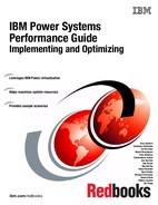
Symmetric multiprocessing (SMP) architecture allows a system to scale beyond one processor. Each processor is connected to the same bus (also known as crossbar switch) to access the main memory. But this computation scaling is not infinite due to the fact that each processor needs to share the same memory bus, so access to the main memory is serialized. With this limitation, this kind of architecture can scale up to four to eight processors only (depending on the hardware).
|
Note: A multicore processor chip can be seen as an SMP system in a chip. All the cores in the same chip share the same memory controller (Figure 2-1).
|
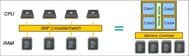
Figure 2-1 SMP architecture and multicore
The Non-Uniform Memory Access (NUMA) architecture is a way to partially solve the SMP scalability issue by reducing pressure on the memory bus.
As opposed to the SMP system, NUMA adds the notion of a multiple memory subsystem called NUMA node:
•Each node is composed of processors sharing the same bus to access memory (a node can be seen as an SMP system).
•NUMA nodes are connected using a special “interlink bus” to provide processor data coherency across the entire system.
Each processor can have access to the entire memory of a system; but access to this memory is not uniform (Figure 2-2 on page 11):
•Access to memory located in the same node (local memory) is direct with a very low latency.
•Access to memory located in another node is achieved through the interlink bus with a higher latency.
By limiting the number of processors that directly access the entire memory, performance is improved compared to an SMP because of the much shorter queue of requests on each memory domain.
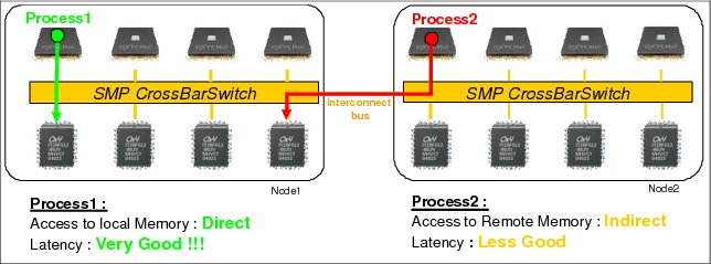
Figure 2-2 NUMA architecture concept
The architecture design of the Power platform is mostly NUMA with three levels:
•Each POWER7 chip has its own memory dimms. Access to these dimms has a very low latency and is named local.
•Up to four POWER7 chips can be connected to each other in the same CEC (or node) by using X, Y, Z buses from POWER7. Access to memory owned by another POWER7 chip in the same CEC is called near or remote. Near or remote memory access has a higher latency compared than local memory access.
•Up to eight CECs can be connected through A, B buses from a POWER7 chip (only on high-end systems). Access to memory owned by another POWER7 in another CEC (or node) is called far or distant. Far or distant memory access has a higher latency than remote memory access.

Figure 2-3 Power Systems with local, near, and far memory access
Summary: Power Systems can have up to three different latency memory accesses (Figure 2-3). This memory access time depends on the memory location relative to a processor.
Latency access time (from lowest to highest): local → near or remote → far or distant.
Many people focus on the latency effect and think NUMA is a problem, which is wrong. Remember that NUMA is attempting to solve the scalability issue of the SMP architecture. Having a system with 32 cores in two CECs performs better than 16 cores in one CEC; check the system performance document at:
2.2.2 PowerVM logical partitioning and NUMA
You know now that the hardware architecture of the IBM Power Systems is based on NUMA. But compared to other systems, Power System servers offer the ability to create several LPARs, thanks to PowerVM.
The PowerVM hypervisor is an abstraction layer that runs on top of the hardware. One of its roles is to assign cores and memory to the defined logical partitions (LPARs). The POWER7 hypervisor was improved to maximize partition performance through processor and memory affinity. It optimizes the assignment of processor and memory to partitions based on system topology. This results in a balanced configuration when running multiple partitions on a system. The first time an LPAR gets activated, the hypervisor allocates processors as close as possible to where allocated memory is located in order to reduce remote and distant memory access. This processor and memory placement is preserved across LPAR reboot (even after a shutdown and reactivation of the LPAR profile) to keep consistent performance and prevent fragmentation of the hypervisor memory.
For shared partitions, the hypervisor assigns a home node domain, the chip where the partition’s memory is located. The entitlement capacity (EC) and the amount of memory determine the number of home node domains for your LPAR. The hypervisor dispatches the shared partition’s virtual processors (VP) to run on the home node domain whenever possible. If dispatching on the home node domain is not possible due to physical processor overcommitment of the system, the hypervisor dispatches the virtual processor temporarily on another chip.
Let us take some example to illustrate the hypervisor resource placement for virtual processors.
In a POWER 780 with four drawers and 64 cores (Example 2-1), we create one LPAR with different EC/VP configurations and check the processor and memory placement.
Example 2-1 POWER 780 configuration
{D-PW2k2-lpar2:root}/home/2bench # prtconf
System Model: IBM,9179-MHB
Machine Serial Number: 10ADA0E
Processor Type: PowerPC_POWER7
Processor Implementation Mode: POWER 7
Processor Version: PV_7_Compat
Number Of Processors: 64
Processor Clock Speed: 3864 MHz
CPU Type: 64-bit
Kernel Type: 64-bit
LPAR Info: 4 D-PW2k2-lpar2
Memory Size: 16384 MB
Good Memory Size: 16384 MB
Platform Firmware level: AM730_095
Firmware Version: IBM,AM730_095
Console Login: enable
Auto Restart: true
Full Core: false
•D-PW2k2-lpar2 is created with EC=6.4, VP=16, MEM=4 GB. Because of EC=6.4, the hypervisor creates one HOME domain in one chip with all the VPs (Example 2-2).
Example 2-2 Number of HOME domains created for an LPAR EC=6.4, VP=16
D-PW2k2-lpar2:root}/ # lssrad -av
REF1 SRAD MEM CPU
0
0 3692.12 0-63
•D-PW2k2-lpar2 is created with EC=10, VP=16, MEM=4 GB. Because of EC=10, which is greater than the number of cores in one chip, the hypervisor creates two HOME domains in two chips with VPs spread across them (Example 2-3).
Example 2-3 Number of HOME domain created for an LPAR EC=10, VP=16
{D-PW2k2-lpar2:root}/ # lssrad -av
REF1 SRAD MEM CPU
0
0 2464.62 0-23 28-31 36-39 44-47 52-55 60-63
1 1227.50 24-27 32-35 40-43 48-51 56-59
•Last test with EC=6.4, VP=64 and MEM=16 GB; just to verify that number of VP has no influence on the resource placement made by the hypervisor.
EC=6.4 < 8 cores so it can be contained in one chip, even if the number of VPs is 64 (Example 2-4).
Example 2-4 Number of HOME domains created for an LPAR EC=6.4, VP=64
D-PW2k2-lpar2:root}/ # lssrad -av
REF1 SRAD MEM CPU
0
0 15611.06 0-255
Of course, it is obvious that 256 SMT threads (64 cores) cannot really fit in one POWER7 8-core chip. lssrad only reports the VPs in front of their preferred memory domain (called home domain).
On LPAR activation, the hypervisor allocates only one memory domain with 16 GB because our EC can be store within a chip (6.4 EC < 8 cores), and there is enough free cores in a chip and enough memory close to it. During the workload, if the need in physical cores goes beyond the EC, the POWER hypervisor tries to dispatch VP on the same chip (home domain) if possible. If not, VPs are dispatched on another POWER7 chip with free resources, and memory access will not be local.
Conclusion
If you have a large number of LPARs on your system, we suggest that you create and start your critical LPARs first, from the biggest to the smallest. This helps you to get a better affinity configuration for these LPARs because it makes it more possible for the POWER hypervisor to find resources for optimal placement.
|
Tip: If you have LPARs with a virtualized I/O card that depend on resources from a VIOS, but you want them to boot before the VIOS to have a better affinity, you can:
1. Start LPARs the first time (most important LPARs first) in “open firmware” or “SMS” mode to let the PowerVM hypervisor assign processor and memory.
2. When all your LPARs are up, you can boot the VIOS in normal mode.
3. When the VIOS are ready, you can reboot all the LPARs in normal mode. The order is not important here because LPAR placement is already optimized by PowerVM in step 1.
|
Even if the hypervisor optimizes your LPAR processor and memory affinity on the very first boot and tries to keep this configuration persistent across reboot, you must be aware that some operations can change your affinity setup, such as:
•Reconfiguration of existing LPARs with new profiles
•Deleting and recreating LPARs
•Adding and removing resources to LPARs dynamically (dynamic LPAR operations)
In the next chapter we show how to determine your LPAR processor memory affinity, and how to re-optimize it.
2.2.3 Verifying processor memory placement
You need now to find a way to verify whether the LPARs created have an “optimal” processor and memory placement, which is achieved when, for a given LPAR definition (number of processors and memory), the partition uses the minimum number of sockets and books to reduce remote and distant memory access to the minimum. The information about your system, such as the number of cores per chip, memory per chip and per book, are critical to be able to make this estimation.
Here is an example for a system with 8-core POWER7 chips, 32 GB of memory per chip, two books (or nodes), and two sockets per node.
•An LPAR with six cores, 24 GB of memory is optimal if it can be contained in one chip (only local memory access).
•An LPAR with 16 cores, 32 GB of memory is optimal if it can be contained in two chips within the same book (local and remote memory access). This is the best processor and memory placement you can have with this number of cores. You must also verify that the memory is well balanced across the two chips.
•An LPAR with 24 cores, 48 GB memory is optimal if it can be contained in two books with a balanced memory across the chips. Even if you have some distant memory access, this configuration is optimal because you do not have another solution to satisfy the 24 required cores.
•An LPAR with 12 cores, 72 GB of memory is optimal if it can be contained in two books with a balanced memory across the chips. Even if you have some distant memory access, this configuration is optimal because you do not have another solution to satisfy the 72 GB of memory.
As explained in the shaded box on page 14, some operations such as dynamic LPAR can “fragment” your LPAR configuration, which gives you some nonoptimal placement for some LPARs. As described in Figure 2-4, avoid having a system with “fragmentation” in the LPAR processor and memory assignment.
Also, be aware that the more LPARs you have, the harder it is to have all your partitions defined with an optimal placement. Sometimes you have to take a decision to choose which LPARs are more critical, and give them a better placement by starting them (the first time) before the others (as explained in 2.2.2, “PowerVM logical partitioning and NUMA” on page 12).
Figure 2-4 Example of optimal versus fragmented LPAR placement
Verifying LPAR resource placement in AIX
In an AIX partition, the lparstat -i command shows how many processors and how much memory are defined in your partition (Example 2-5).
Example 2-5 Determining LPAR resource with lparstat
{D-PW2k2-lpar1:root}/ # lparstat -i
Node Name : D-PW2k2-lpar1
Partition Name : D-PW2k2-lpar1
Partition Number : 3
Type : Dedicated-SMT-4
Mode : Capped
Entitled Capacity : 8.00
Partition Group-ID : 32771
Shared Pool ID : -
Online Virtual CPUs : 8
Maximum Virtual CPUs : 16
Minimum Virtual CPUs : 1
Online Memory : 32768 MB
Unallocated I/O Memory entitlement : -
Memory Group ID of LPAR : -
Desired Virtual CPUs : 8
Desired Memory : 32768 MB
....
From Example 2-5 on page 15, we know that our LPAR has eight dedicated cores with SMT4 (8x4=32 logical cpu) and 32 GB of memory.
Our system is a 9179-MHB (POWER 780) with four nodes, two sockets per node, each socket with eight cores and 64 GB of memory. So, the best resource placement for our LPAR would be one POWER7 chip with eight cores and 32 GB of memory next to this chip.
To check your processor and memory placement, you can use the lssrad -av command from your AIX instance, as shown in Example 2-6.
Example 2-6 Determining resource placement with lssrad
{D-PW2k2-lpar1:root}/ # lssrad -av
REF1 SRAD MEM CPU
0
0 15662.56 0-15
1
1 15857.19 16-31
•REF1 (first hardware-provided reference point) represents a drawer of our POWER 780. For a POWER 795, this represents a book. Systems other than POWER 770, POWER 780, or POWER 795, do not have a multiple drawer configuration (Table 1-1 on page 3) so they cannot have several REF1s.
•Scheduler Resource Allocation Domain (SRAD) represents a socket number. In front of each socket, there is an amount of memory attached to our partition. We also find the logical processor number attached to this socket.
|
Note: The number given by REF1 or SRAD does not represent the real node number or socket number on the hardware. All LPARs will report a REF1 0 and a SRAD 0. They just represent a logical number inside the operating system instance.
|
From Example 2-6, we can conclude that our LPAR is composed of two sockets (SRAD 0 and 1) with four cores on each (0-15 = 16-31 = 16 lcpu SMT4 = 4 cores) and 16 GB of memory attached to each socket. These two sockets are located in two different nodes (REF1 0 and 1).
Compared to our expectation (which was: only one socket with 32 GB of memory means only local memory access), we have two different sockets in two different nodes (high potential of distant memory access). The processor and memory resource placement for this LPAR is not optimal and performance could be degraded.
LPAR processor and memory placement impact
To demonstrate the performance impact, we performed the following experiment: We created an LPAR (eight dedicated cores, 32 GB of memory) on a POWER 780 (four drawers, eight sockets). We generated an OnLine Transactional Processing (OLTP) load on an Oracle database with 200 concurrent users and measured the number of transactions per second (TPS). Refer to the “Oracle SwingBench” on page 342.
Test 1: The first test was done with a nonoptimal resource placement: eight dedicated cores spread across two POWER7 chips, as shown in Example 2-6,
Test 2: The second test was done with an optimal resource placement: eight dedicated cores on the same chip with all the memory attached as shown in Example 2-7 on page 17.
Example 2-7 Optimal resource placement for eight cores and 32 GB of memory
{D-PW2k2-lpar1:root}/ # lssrad -av
REF1 SRAD MEM CPU
0
0 31519.75 0-31
Test results
During the two tests, the LPAR processor utilization was 100%. We waited 5 minutes during the steady phase and took the average TPS as result of the experiment (Table 2-1 on page 18). See Figure 2-5, and Figure 2-6.

Figure 2-5 Swinbench results for test1 (eight cores on two chips: nonoptimal resource placement)

Figure 2-6 Swingbench results for Test 2 (eight cores on one chip: optimal resource placement)
This experiment shows 24% improvement in TPS when most of the memory accesses are local compared to a mix of 59% local and 41% distant. This is confirmed by a higher Cycle per Instruction (CPI) in test 1 (CPI=7.5) compared to test 2 (CPI=4.8). This difference can be explained by a higher memory latency for 41% of the access in test 1, which causes some additional empty processor cycle when waiting for data from the distant memory to complete the instruction.
Table 2-1 Result table of resource placement impact test on an Oracle OLTP workload
|
Test name
|
Resource
placement
|
Access to local
memory1
|
CPI
|
Average TPS
|
Performance ratio
|
|
Test 1
|
non Optimal
(local + distant)
|
59%
|
7.5
|
5100
|
1.00
|
|
Test 2
|
Optimal
(only local)
|
99.8%
|
4.8
|
6300
|
1.24
|
Notice that 59% local access is not so bad with this “half local/ half distant” configuration. This is because the AIX scheduler is aware of the processor and memory placement in the LPAR, and has enhancements to reduce the NUMA effect as shown in 6.1, “Optimizing applications with AIX features” on page 280.
|
Note: These results are from experiments based on a load generation tool named Swingbench; results may vary depending on the characteristics of your workload. The purpose of this experiment is to give you an idea of the potential gain you can get if you take care of your resource placement.
|
2.2.4 Optimizing the LPAR resource placement
As explained in the previous section, processor and memory placement can have a direct impact on the performance of an application. Even if the PowerVM hypervisor optimizes the resource placement of your partitions on the first boot, it is still not “clairvoyant.” It cannot know by itself which partitions are more important than others, and cannot anticipate what will be the next changes in our “production” (creation of new “critical production” LPARs, deletion of old LPARs, dynamic LPAR, and so on). You can help the PowerVM hypervisor to cleanly place the partitions by sizing your LPAR correctly and using the proper PowerVM option during your LPAR creation.
Do not oversize your LPAR
Realistic sizing of your LPAR is really important to get a better processor memory affinity. Try not to give to a partition more processor than needed.
If a partition has nine cores assigned, cores and memory are spread across two chips (best scenario). If, during peak time, this partition consumes only seven cores, it would have been more efficient to assign seven or even eight cores to this partition only to have the cores and the memory within the same POWER7 chip.
For a virtualized processor, a good Entitlement Capacity (EC) is really important. Your EC must fit with the average need of processor power of your LPAR during a regular load (for example, the day only for a typical day’s OLTP workload, the night only for typical night “batch” processing). This gives you a resource placement that better fits the needs of your partition. As for dedicated processor, try not to oversize your EC across domain boundaries (cores per chip, cores per node). A discussion regarding how to efficiently size your virtual processor resources is available in 3.1, “Optimal logical partition (LPAR) sizing” on page 42.
Memory follows the same rule. If you assign to a partition more memory than can be found behind a socket or inside a node, you will have to deal with some remote and distant memory access. This is not a problem if you really need this memory, but if you do not use it totally, this situation could be avoided with a more realistic memory sizing.
Affinity groups
This option is available with PowerVM Firmware level 730. The primary objective is to give hints to the hypervisor to place multiple LPARs within a single domain (chip, drawer, or book). If multiple LPARs have the same affinity_group_id, the hypervisor places this group of LPARs as follows:
•Within the same chip if the total capacity of the group does not exceed the capacity of the chip
•Within the same drawer (node) if the capacity of the group does not exceed the capacity of the drawer
The second objective is to give a different priority to one or a group of LPARs. Since Firmware level 730, when a server frame is rebooted, the hypervisor places all LPARs before their activation. To decide which partition (or group of partitions) should be placed first, it relies on affinity_group_id and places the highest number first (from 255 to 1).
The following Hardware Management Console (HMC) CLI command adds or removes a partition from an affinity group:
chsyscfg -r prof -m <system_name> -i name=<profile_name>,lpar_name=<partition_name>,affinity_group_id=<group_id>
where group_id is a number between 1 and 255, affinity_group_id=none removes a partition from the group.
The command shown in Example 2-8 sets the affinty_group_id to 250 to the profile named Default for the 795_1_AIX1 LPAR.
Example 2-8 Modifying the affinity_group_id flag with the HMC command line
hscroot@hmc24:~> chsyscfg -r prof -m HAUTBRION -i name=Default,lpar_name=795_1_AIX1,affinity_group_id=250
You can check the affinity_group_id flag of all the partitions of your system with the lsyscfg command, as described in Example 2-9.
Example 2-9 Checking the affinity_group_id flag of all the partitions with the HMC command line
hscroot@hmc24:~> lssyscfg -r lpar -m HAUTBRION -F name,affinity_group_id
p24n17,none
p24n16,none
795_1_AIX1,250
795_1_AIX2,none
795_1_AIX4,none
795_1_AIX3,none
795_1_AIX5,none
795_1_AIX6,none
POWER 795 SPPL option and LPAR placement
On POWER 795, there is an option called Shared Partition Processor Limit (SPPL). Literally, this option limits the processor capacity of an LPAR. By default, this option is set to 24 for POWER 795 with six-core POWER7 chip or 32 for the eight-core POWER7 chip. If your POWER 795 has three processor books or more, you can set this option to maximum to remove this limit. This change can be made on the Hardware Management Console (HMC).

Figure 2-7 Changing POWER 795 SPPL option from the HMC
|
Changing SPPL on the Hardware Management Console (HMC): Select your POWER 795 → Properties → Advanced → change Next SPPL to maximum (Figure 2-7). After changing the SPPL value, you need to stop all your LPARs and restart the POWER 795.
|
The main objective of the SPPL is not to limit the processor capacity of an LPAR, but to influence the way the PowerVM hypervisor assigns processor and memory to the LPARs.
•When SPPL is set to 32 (or 24 if six-core POWER7), then the PowerVM hypervisor allocates processor and memory in the same processor book, if possible. This reduces access to distant memory to improve memory latency.
•When SPPL is set to maximum, there is no limitation to the number of desired processors in your LPAR. But large LPAR (more than 24 cores) will be spread across several books to use more memory DIMMs and maximize the interconnect bandwidth. For example, a 32-core partition in SPPL set to maximum will spread across two books compared to only one if SPPL is set to 32.
SPPL maximum improves memory bandwidth for large LPARs, but reduces locality of the memory. This can have a direct impact on applications that are more latency sensitive compared to memory bandwidth (for example, databases for most of the client workload).
To address this case, a flag can be set on the profile of each large LPAR to signal the hypervisor to try to allocate processor and memory in a minimum number of books (such as SPPL 32 or 24). This flag is lpar_placement and can be set with the following HMC command (Example 2-10 on page 21):
chsyscfg -r prof -m <managed-system> -i name=<profile-name>,lpar_name=<lpar-name>,lpar_placement=1
Example 2-10 Modifying the lpar_placement flag with the HMC command line
This command sets the lpar_placement to 1 to the profile named default for 795_1_AIX1 LPAR:
hscroot@hmc24:~> chsyscfg -r prof -m HAUTBRION -i name=Default,lpar_name=795_1_AIX1,lpar_placement=1
You can use the lsyscfg command to check the current lpar_placement value for all the partitions of your system:
hscroot@hmc24:~> lssyscfg -r lpar -m HAUTBRION -F name,lpar_placement
p24n17,0
p24n16,0
795_1_AIX1,1
795_1_AIX2,0
795_1_AIX4,0
795_1_AIX3,0
795_1_AIX5,0
795_1_AIX6,0
Table 2-2 describes in how many books an LPAR is spread by the hypervisor, depending on the number of processors of this LPAR, SPPL value, and lpar_placement value.
Table 2-2 Number of books used by LPAR depending on SPPL and the lpar_placement value
|
Number of processors
|
Number of books
(SPPL=32)
|
Number of books
(SPPL=maximum,
lpar_placement=0)
|
Number of books
(SPPL=maximum,
lpar_placement=1)
|
|
8
|
1
|
1
|
1
|
|
16
|
1
|
1
|
1
|
|
24
|
1
|
1
|
1
|
|
32
|
1
|
2
|
1
|
|
64
|
not possible
|
4
|
2
|
|
Note: The lpar_placement=1 flag is only available for PowerVM Hypervisor eFW 730 and above. In the 730 level of firmware, lpar_placement=1 was only recognized for dedicated processors and non-TurboCore mode (MaxCore) partitions when SPPL=MAX.
Starting with the 760 firmware level, lpar_placement=1 is also recognized for shared processor partitions with SPPL=MAX or systems configured to run in TurboCore mode with SPPL=MAX.
|
Force hypervisor to re-optimize LPAR resource placement
As explained in 2.2.2, “PowerVM logical partitioning and NUMA” on page 12, the PowerVM hypervisor optimizes resource placement on the first LPAR activation. But some operations, such as dynamic LPAR, may result in memory fragmentation causing LPARs to be spread across multiple domains. Because the hypervisor keeps track of the placement of each LPAR, we need to find a way to re-optimize the placement for some partitions.
|
Note: In this section, we give you some ways to force the hypervizor to re-optimize processor and memory affinity. Most of these solutions are workarounds based on the new PowerVM options in Firmware level 730.
In Firmware level 760, IBM gives an official solution to this problem with Dynamic Platform Optimizer (DPO). If you have Firmware level 760 or above, go to “Dynamic Platform Optimizer” on page 23.
|
There are three ways to re-optimize LPAR placement, but they can be disruptive:
•You can shut down all your LPARs, and restart your system. When PowerVM hypervisor is restarted, it starts to place LPARs starting from the higher group_id to the lower and then place LPARs without affinity_group_id.
•Shut down all your LPARs and create a new partition in an all-resources mode and activate it in open firmware. This frees all the resources from your partitions and re-assigns them to this new LPAR. Then, shut down the all-resources and delete it. You can now restart your partitions. They will be re-optimized by the hypervisor. Start with the most critical LPAR to have the best location.
•There is a way to force the hypervisor to forget placement for a specific LPAR. This can be useful to get processor and memory placement from noncritical LPARs, and force the hypervisor to re-optimize a critical one. By freeing resources before re-optimization, your critical LPAR will have a chance to get a better processor and memory placement.
– Stop critical LPARs that should be re-optimized.
– Stop some noncritical LPARs (to free the most resources possible to help the hypervisor to find a better placement for your critical LPARs).
– Freeing resources from the non-activated LPARs with the following HMC commands. You need to remove all memory and processors (Figure 2-8):
chhwres -r mem -m <system_name> -o r -q <num_of_Mbytes> --id <lp_id>
chhwres -r proc -m <system_name> -o r --procunits <number> --id <lp_id>
You need to remove all memory and processor as shown in Example 2-11.
You can check the result from the HMC. All resources “Processing Units” and Memory should be 0, as shown in Figure 2-9 on page 23.
– Restart your critical LPAR. Because all processors and memory are removed from your LPAR, the PowerVM hypervisor is forced to re-optimize the resource placements for this LPAR.
– Restart your noncritical LPAR.

Figure 2-8 HMC screenshot before freeing 750_1_AIX1 LPAR resources
Example 2-11 HMC command line to free 750_1_AIX1 LPAR resources
hscroot@hmc24:~> chhwres -r mem -m 750_1_SN106011P -o r -q 8192 --id 10
hscroot@hmc24:~> chhwres -r proc -m 750_1_SN106011P -o r --procunits 1 --id 10
Figure 2-9 HMC screenshot after freeing 750_1_AIX1 LPAR resources
In Figure 2-9, notice that Processing Units and Memory of the 750_1_AIX1 LPAR are now set to 0. This means that processor and memory placement for this partition will be re-optimized by the hypervisor on the next profile activation.
Dynamic Platform Optimizer
Dynamic Platform Optimizer (DPO) is a new capability of IBM Power Systems introduced with Firmware level 760, and announced in October 2012. It is free of charge, available since October 2012 for POWER 770+, POWER 780+, and since November 2012 for POWER 795. Basically it allows the hypervisor to dynamically optimize the processor and memory resource placement of LPARs while they are running (Figure 2-10). This operation needs to be run manually from the HMC command line.

Figure 2-10 DPO defragmentation illustration
To check whether your system supports DPO: Select your system from your HMC graphical interface:

Figure 2-11 Checking for DPO in system capabilities
Dynamic Platform Optimizer is able to give you a score (from 0 to 100) of the actual resource placement in your system based on hardware characteristics and partition configuration. A score of 0 means poor affinity and 100 means perfect affinity.
|
Note: Depending on the system topology and partition configuration, perfect affinity is not always possible.
|
On the HMC, the command line to get this score is:
lsmemopt -m <system_name> -o currscore
In Example 2-12, you can see that our system affinity is 75.
Example 2-12 HMC DPO command to get system affinity current score
hscroot@hmc56:~> lsmemopt -m Server-9117-MMD-SN101FEF7 -o currscore
curr_sys_score=75
From the HMC, you can also ask for an evaluation of what the score on your system would be after affinity was optimized using the Dynamic Platform Optimizer.
|
Note: The predicted affinity score is an estimate, and may not match the actual affinity score after DPO has been run.
|
The HMC command line to get this score is:
lsmemopt -m <system_name> -o calcscore
In Example 2-13 on page 25, you can see that our current system affinity score is 75, and 95 is predicted after re-optimization by DPO.
Example 2-13 HMC DPO command to evaluate affinity score after optimization
hscroot@hmc56:~> lsmemopt -m Server-9117-MMD-SN101FEF7 -o calcscore
curr_sys_score=75,predicted_sys_score=95,"requested_lpar_ids=5,6,7,9,10,11,12,13,14,15,16,17,18,19,20,21,22,23,24,25,27,28,29,30,31,32,33,34,35,36,37,38,41,42,43,44,45,46,47,53",protected_lpar_ids=none
When DPO starts the optimization procedure, it starts with LPARs from the highest affinity_group_id from id 255 to 0 (see “Affinity groups” on page 19), then it continues with the biggest partition and finishes with the smallest one.
To start affinity optimization with DPO for all partitions in your system, use the following HMC command:
optmem -m <system_name> -o start -t affinity
|
Note: The optmem command-line interface supports a set of “requested” partitions, and a set of “protected” partitions. The requested ones are prioritized highest. The protected ones are not touched. Too many protected partitions can adversely affect the affinity optimization, since their resources cannot participate in the system-wide optimization.
|
To perform this operation, DPO needs free memory available in the system and some processor cycles. The more resources available for DPO to perform its optimization, the faster it will be. But be aware that this operation can take time and performance could be degraded; so this operation should be planned during low activity periods to reduce the impact on your production environment.
|
Note: Some functions such as dynamic LPAR and Live Partition Mobility cannot run concurrently with the optimizer.
|
Here are a set of examples to illustrate how to start (Example 2-14), monitor (Example 2-15) and stop (Example 2-16) a DPO optimization.
Example 2-14 Starting DPO on a system
hscroot@hmc56:~> optmem -m Server-9117-MMD-SN101FEF7 -o start -t affinity
Example 2-15 Monitoring DPO task progress
hscroot@hmc56:~> lsmemopt -m Server-9117-MMD-SN101FEF7
in_progress=0,status=Finished,type=affinity,opt_id=1,progress=100,
requested_lpar_ids=non,protected_lpar_ids=none,”impacted_lpar_ids=106,110”
Example 2-16 Forcing DPO to stop before the end of optimization
hscroot@hmc56:~> optmem -m Server-9117-MMD-SN101FE_F7 -o stop
|
Note: Stopping DPO before the end of the optimization process can result in poor affinity for some partitions.
|
Partitions running on AIX 7.1 TL2, AIX 6.1 TL8, and IBM i 7.1 PTF MF56058 receive notification from DPO when the optimization completes, and whether affinity has been changed for them. This means that all the tools such as lssrad (Example 2-6 on page 16) can report the changes automatically; but more importantly, the scheduler in these operating systems is now aware of the new processor and memory affinity topology.
For older operating systems, the scheduler will not be aware of the affinity topology changes. This could result in performance degradation. You can exclude these partitions from the DPO optimization to avoid performance degradation by adding them to the protected partition set on the optmem command, or reboot the partition to refresh the processor and memory affinity topology.
2.2.5 Conclusion of processor and memory placement
As you have seen, processor and memory placement is really important when talking about raw performance. Even if the hypervisor optimizes the affinity, you can influence it and help it by:
•Knowing your system hardware architecture and planning your LPAR creation.
•Creating and starting critical LPARs first.
•Giving a priority order to your LPAR and correctly setting the affinity_group HMC parameter.
•Setting the parameter lpar_placement when running on POWER 795 with SSPL=maximum.
•If possible, use DPO to defragment your LPAR placement and optimize your system.
If you want to continue this Processor and Memory Affinity subject at the AIX operating system level, refer to 6.1, “Optimizing applications with AIX features” on page 280.
2.3 Performance consequences for I/O mapping and adapter placement
In this section, we provide adapter placement, which is an important step to consider when installing or expanding a server.
Environments change all the time, in every way, from a simple hardware upgrade to entire new machines, and many details come to our attention.
Different machines have different hardware, even when talking about different models of the same type. The POWER7 family has different types and models from the entry level to high-end purposes and the latest POWER7 models may have some advantages over their predecessors. If you are upgrading or acquiring new machines, the same plan used to deploy the first may not be the optimal for the latest.
Systems with heavy I/O workloads demand machines capable of delivering maximum throughput and that depends on several architectural characteristics and not only on the adapters themselves. Buses, chipsets, slots—all of these components must be considered to achieve maximum performance. And due to the combination of several components, maximum performance may not be the same that some of them offer individually.
These technologies are always being improved to combine the maximum throughput, but one of the key points for using them efficiently and to achieve good performance is how they are combined, and sometimes this can be a difficult task.
Each machine type has a different architecture and an adequate setup is required to obtain the best I/O throughput from that server. Because the processors and chipsets are connected through different buses, the way adapters are distributed across the slots on a server directly affects the I/O performance of the environment.
Connecting adapters in the wrong slots may not give you the best performance because you do not take advantage of the hardware design, and worse, it may even cause performance degradation. Even different models of the same machine type may have important characteristics for those who want to achieve the highest performance and take full advantage of their environments.
|
Important: Placing the wrong card in the wrong slot may not only not bring you the performance that you are expecting but can also degrade the performance of your existing environment.
|
To illustrate some of the differences that can affect the performance of the environment, we take a look at the design of two POWER 740 models. In the sequence, we make a brief comparison between the POWER 740 and the POWER 770, and finally between two models of the POWER 770.
|
Note: The next examples are only intended to demonstrate how the designs and architectures of the different machines can affect the system performance. For other types of machines, make sure you read the Technical Overview and Introduction documentation for that specific model, available on the IBM Hardware Information Center at:
http://pic.dhe.ibm.com/infocenter/powersys/v3r1m5/index.jsp
|
2.3.1 POWER 740 8205-E6B logical data flow
Figure 2-12 on page 28 presents the logical data flow of the 8205-E6B (POWER 740), one of the smaller models of the POWER7 family.

Figure 2-12 POWER 740 8205-E6B - Logic unit flow
The 8205-E6B has two POWER7 chips, each with two GX controllers (GX0 and GX1) connected to the GX++ slots 1 and 2 and to the internal P5-IOC2 controller. The two GX++ bus slots provide 20 Gbps bandwidth for the expansion units while the P5-IOC2 limits the bandwidth of the internal slots to 10 GBps only. Further, the GX++ Slot 1 can connect both an additional P5-IOC2 controller and external expansion units at the same time, sharing its bandwidth, while GX++ Slot 2 only connects to external expansion units.
Notice that this model also has the Integrated Virtual Ethernet (IVE) ports connected to the P5-IOC2, sharing the same bandwidth with all the other internal adapters and SAS disks. It also has an External SAS Port, allowing for more weight over the 10 Gbps chipset.
2.3.2 POWER 740 8205-E6C logical data flow
This is the same picture as seen in the previous section but this time, we have the successor model 8205-E6C, as shown in Figure 2-13 on page 29.

Figure 2-13 POWER 740 8205-E6C - Logic unit flow
Although the general organization of the picture is a bit different, the design itself is still the same, but in this version there a few enhancements to notice. First, the 1.25 GHz P5-IOC from the 8205-E6B has been upgraded to the new P7-IOC with a 2.5 GHz clock on 8205-E6C, raising the channel bandwidth from 10 Gbps to 20 Gbps. Second, the newest model now comes with PCIe Gen2 slots, which allows peaks of 4 Gbps for x8 interfaces instead of the 2 Gbps of their predecessors.
Another interesting difference in this design is that the GX++ slots have been flipped. The GX slot connected to the POWER7 Chip 2 now is the GX++ Slot 1, which provides dedicated channel and bandwidth to the expansion units. And the POWER7 Chip 1 keeps the two separate channels for the P7-IOC and the GX++ Slot 2, which can still connect an optional P7-IOC bus with the riser card.
Finally, beyond the fact that the P7-IOC has an increased bandwidth over the older P5-IOC2, the 8205-E6C does not come with the External SAS Port (although it is allowed through adapter expansion), neither the Integrated Virtual Ethernet (IVE) ports, constraining the load you can put on that bus.
|
Important: To take full advantage of the PCIe Gen2 slot’s characteristics, compatible PCIe2 cards must be used. Using the old PCIe Gen1 cards on Gen2 slots is supported, but although a slight increase of performance may be observed due to the several changes along the bus, the PCIe Gen1cards are still limited to their own speed by design and should not be expected to achieve the same performance as the PCIe Gen2 cards.
|
2.3.3 Differences between the 8205-E6B and 8205-E6C
Table 2-3 gives a clear view of the differences we mentioned.
Table 2-3 POWER 740 comparison - Models 8205-E6B and 8205-E6C
|
POWER 740
|
8205-E6B
|
8205-E6C
|
|
GX++ Slots
|
2x 20 Gbps
|
2x 20 Gbps
|
|
Internal I/O chipset
|
P5-IOC2 (10 Gbps)
|
P7-IOC (20 Gbps)
|
|
PCIe Version
|
Gen1 (2 Gbps)
|
Gen2 (4 Gbps), Gen1-compatible
|
|
Primary GX++ Slot
|
POWER7 Chip 1 (shared bandwidth)
|
POWER7 Chip 2 (dedicated bandwidth)
|
|
Secondary GX++ Slot
|
POWER7 Chip2 (dedicated bandwidth)
|
POWER7 Chip 1 (shared bandwidth)
|
|
Expansion I/O w/ Riser Card
|
POWER7 Chip 1
|
POWER7 Chip 1
|
The purpose of this quick comparison is to illustrate important differences that exist among the different machines that may go unnoticed when the hardware is configured. You may eventually find out that instead of placing an adapter on a CEC, you may take advantage of attaching it to an internal slot, if your enclosure is not under a heavy load.
2.3.4 POWER 770 9117-MMC logical data flow
Now we take a brief look to another machine type, and you notice that several differences exist between the POWER 740 and the POWER 770.

Figure 2-14 POWER 770 9117-MMC - Logic data flow
As shown in Figure 2-14, the 9117-MMC has a completely different design of the buses. It now has two P7-IOC chipsets by default and one of them is dedicated to four PCIe Gen2 slots. Moreover, both P7-IOCs are exclusively connected to the POWER7 Chip1 while both GX++ slots are exclusively connected to the POWER7 Chip2.
2.3.5 POWER 770 9117-MMD logical data flow
As of the time of this writing, the 9117-MMD model featuring the new POWER7+ processors has recently been announced and once again, along with new features and improvements, a new design has come, as we can see in Figure 2-15 on page 32.
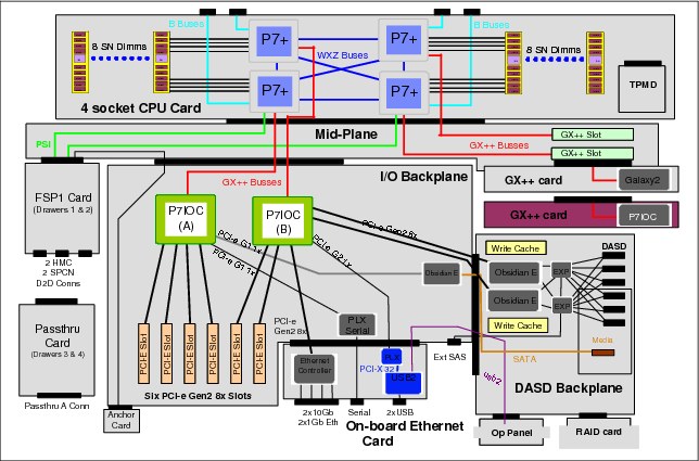
Figure 2-15 POWER 770 9117-MMD - Logic data flow
The 9117-MMD now includes four POWER7+ sockets and for the sake of this section, the major improvement in the design of this model is that the bus sharing has been reduced for the P7-IOC chipsets and the GX++ controllers by connecting each of these controllers to a different socket.
Table 2-4 POWER 770 comparison - Models 9117-MMC and 9117-MMD
|
POWER 770
|
9117-MMC
|
9117-MMD
|
|
Sockets per card
|
2
|
4
|
|
I/O Bus Controller
|
2x P7-IOC (20 Gbps), sharing the same chip.
|
2x P7-IOC (20 Gbps), independent chips.
|
|
GX++ slots (primary and secondary)
|
2x GX++ channels, sharing the same chip.
|
2x GX++ channels, independent chips.
|
Once again, this comparison (Table 2-4) illustrates the hardware evolution in the same type of machines.
2.3.6 Expansion units
Expansion units, as the name says, allow for capacity expansion by providing additional adapters and disk slots. These units are connected to the GX++ slots by using SPCN and 12x cables in specific configurations not covered in this book. These types of connections are designed for minimum latency but still, the more distant the adapters are from the processors, the more latency is present.
Adapters, cables and enclosures are available with Single Data Rate (SDR) and Double Data Rate (DDR) capacity. Table 2-5 shows the bandwidth differences between these two types.
Table 2-5 InfiniBand bandwidth table
|
Connection type
|
Bandwidth
|
Effective
|
|
Single Data Rate (SDR)
|
2.5 Gbps
|
2 Gbps
|
|
Double Data Rate (DDR)
|
5 Gbps
|
4 Gbps
|
In order to take full advantage of DDR, the three components (GX++ adapter, cable, and unit) must be equally capable of transmitting data at that same rate. If any of the components is SDR only, then the communication channel is limited to SDR speed.
|
Note: Detailed information about the several available Expansion Units can be obtained on the IBM Hardware Information Center at:
http://pic.dhe.ibm.com/infocenter/powersys/v3r1m5/index.jsp
|
2.3.7 Conclusions
First, the workload requirements must be known and should be established. Defining the required throughput on an initial installation is quite hard because usually you deal with several aspects that can make such analysis more difficult, but when expanding a system, that is data that can be very useful.
Starting at the choice of the proper machine type and model, all of the hardware characteristics should be carefully studied, deciding on adapter placement to obtain optimal results in accordance with the workload requirements. Even proper cabling has its importance.
At the time of partition deployment, assuming that the adapters have been distributed in the optimal way, assigning the correct slots to the partitions based on their physical placement is another important step to match the proper workload. Try to establish which partitions are more critical in regard to each component (processor, memory, disk, and network) and with that in mind plan their distribution and placement of resources.
|
Note: Detailed information about each machine type and further adapter placement documentation can be obtained in the Technical Overview and Introduction and PCI Adapter Placement documents, available on the IBM Hardware Information Center at:
http://pic.dhe.ibm.com/infocenter/powersys/v3r1m5/index.jsp
|
2.4 Continuous availability with CHARM
IBM continues to introduce new and advanced continuous Reliability, Availability, and Serviceability (RAS) functions in the IBM Power Systems to improve overall system availability. With advanced functions in fault resiliency, recovery, and redundancy design, the impact to the system from hardware failure has been significantly reduced.
With these system attributes, Power Systems continue to be leveraged for server consolidation. For clients experiencing rapid growth in computing needs, upgrading hardware capacity incrementally with limited disruption becomes an important system capability.
In this section we provide a brief overview of the CEC level functions and operations, called CEC Hot Add and Repair Maintenance (CHARM) functions and the POWER 770/780/795 servers that these functions are supporting. The CHARM functions provide the ability to upgrade system capacity and repair the CEC, or the heart of a large computer, without powering down the system.
The CEC hardware includes the processors, memory, I/O hubs (GX adapters), system clock, service processor, and associated CEC support hardware. The CHARM functions consist of special hardware design, service processor, hypervisor, and Hardware Management Console (HMC) firmware. The HMC provides the user interfaces for the system administrator and System Service Representative (SSR) to perform the tasks for the CHARM operation.
2.4.1 Hot add or upgrade
In this section we describe how to work with nodes during add or upgrade operations.
Hot node add
This function allows the system administrator to add a node to a system to increase the processor, memory, and I/O capacity of the system. After the physical node installation, the system firmware activates and integrates the new node hardware into the system.
The new processor and memory resources are available for the creation of new partitions or to be dynamically added to existing partitions. After the completion of the node add operation, additional I/O expansion units can be attached to the new GX adapters in the new node in a separate concurrent I/O expansion unit add operation.
Hot node upgrade (memory)
This function enables an SSR to increase the memory capacity in a system by adding additional memory DIMMs to a node, or upgrading (exchanging) existing memory with higher-capacity memory DIMMs.
The system must have two or more nodes to utilize the hot node upgrade function. Since the node that is being upgraded is functional and possibly running workloads prior to starting the hot upgrade operation, the system administrator uses the “Prepare for Hot Repair or Upgrade” utility, system management tools and operating system (OS) tools to prepare the node for evacuation.
During the hot node upgrade operation, the system firmware performs the node evacuation by relocating the workloads from the target node to other nodes in the system and logically isolating the resources in the target node.
It then deactivates and electrically isolates the node to allow the removal of the node for the upgrade. After the physical node upgrade, the system firmware activates and integrates the node hardware into the system with additional memory.
After the completion of a hot node upgrade operation, the system administrator then restores the usage of processor, memory, and I/O resources, including redundant I/O configurations if present. The new memory resources are available for the creation of new partitions or to be dynamically added to existing partitions by the system administrator using dynamic LPAR operations.
Concurrent GX adapter add
This function enables an SSR to add a GX adapter to increase the I/O capacity of the system. The default settings allow one GX adapter to be added concurrently with a POWER 770/780 system and two GX adapters to be added concurrently to a POWER 795 system, without planning for a GX memory reservation.
After the completion of the concurrent GX adapter add operation, I/O expansion units can be attached to the new GX adapter through separate concurrent I/O expansion unit add operations.
2.4.2 Hot repair
In this section, we describe the hot repair functionality of the IBM POWER Systems servers.
Hot node repair
This function allows an SSR to repair defective hardware in a node of a system while the system is powered on.
The system must have two or more nodes to utilize the hot node repair function. Since the node that is being repaired may be fully or partially functional and running workloads prior to starting the hot repair operation, the system administrator uses the “Prepare for Hot Repair or Upgrade” utility, system management tools and OS tools to prepare the system. During the hot node repair operation, the system firmware performs the node evacuation by relocating workloads in the target node to other nodes in the system and logically isolating the resources in the target node.
It then deactivates and electrically isolates the node to allow the removal of the node for repair. After the physical node repair, the system firmware activates and integrates the node hardware back into the system.
Hot GX adapter repair
This function allows an SSR to repair a defective GX adapter in the system. The GX adapter may still be in use prior to starting the hot repair operation, so the system administrator uses the “Prepare for Hot Repair or Upgrade” utility and OS tools to prepare the system.
During the hot GX repair operation, the system firmware logically isolates the resources associated with or dependent on the GX adapter, then deactivates and electrically isolates the GX adapter to allow physical removal for repair.
After the completion of the hot repair operation, the system administrator restores the usage of I/O resources, including redundant I/O configurations if present.
Concurrent system controller repair
The concurrent System Controller (SC) repair function allows an SSR to concurrently replace a defective SC card. The target SC card can be fully or partially functional and in the primary or backup role, or it can be in a nonfunctional state.
After the repair, the system firmware activates and integrates the new SC card into the system in the backup role.
2.4.3 Prepare for Hot Repair or Upgrade utility
The Prepare for Hot Repair or Upgrade (PHRU) utility is a tool on the HMC used by the system administrator to prepare the system for a hot node repair, hot node upgrade, or hot GX adapter repair operation.
Among other things, the utility identifies resources that are in use by operating systems and must be deactivated or released by the operating system. Based on the PHRU utility's output, the system administrator may reconfigure or vary off impacted I/O resources using operating system tools, remove reserved processing units from shared processor pools, reduce active partitions' entitled processor and/or memory capacity using dynamic LPAR operations, or shut down low priority partitions.
This utility also runs automatically near the beginning of a hot repair or upgrade procedure to verify that the system is in the proper state for the procedure. The system firmware does not allow the CHARM operation to proceed unless the necessary resources have been deactivated and/or made available by the system administrator and the configuration supports it.
Table 2-6 summarizes the usage of the PHRU utility based on specific CHARM operations and expected involvement of the system administrator and service representative.
Table 2-6 PHRU utility usage
|
CHARM operation
|
Minimum # of
nodes to use
operation
|
PHRU usage
|
System
administrator
|
Service
representative
|
|
Hot Node Add
|
1
|
No
|
Planning only
|
Yes
|
|
Hot Node Repair
|
2
|
Yes
|
Yes
|
Yes
|
|
Hot Node Upgrade
(memory)
|
2
|
Yes
|
Yes
|
Yes
|
|
Concurrent GX
Adapter Add
|
1
|
No
|
Planning only
|
Yes
|
|
Hot GX Adapter
Repair
|
1
|
Yes
|
Yes
|
Yes
|
|
Concurrent System
Controller Repair
|
1
|
No
|
Planning only
|
Yes
|
2.4.4 System hardware configurations
To obtain the maximum system and partition availability benefits from the CEC Hot Add and Repair Maintenance functions, follow these best practices and guidelines for system hardware configuration:
•Request the free pre-sales “I/O Optimization for RAS” services offering to ensure that your system configuration is optimized to minimize disruptions when using CHARM.
•The system should have spare processor and memory capacity to allow a node to be taken offline for hot repair or upgrade with minimum impact and memory capacity to take the node offline.
•All critical I/O resources should be configured using an operating system multipath I/O redundancy configuration.
•Redundant I/O paths should be configured through different nodes and GX adapters.
•All logical partitions should have RMC network connections with the HMCs.
•The HMC should be configured with redundant service networks with both service processors in the CEC.
|
Note: Refer to the IBM POWER 770/780 and 795 Servers CEC Hot Add and Repair Maintenance Technical Overview at:
|
2.5 Power management
One of the new features introduced with the POWER6 family of servers was Power Management. This feature is part of the IBM EnergyScale™ technology featured on the POWER6 processor. IBM EnergyScale provides functions to help monitor and optimize hardware power and cooling usage. While the complete set of IBM EnergyScale is facilitated through the IBM Systems Director Active Energy Manager™, the Power Management option can also be enabled in isolation from the HMC or ASMI interface.
The feature is known on the HMC GUI as Power Management and Power Saver mode on the ASMI GUI; while in IBM EnergyScale terminology it is referred to as Static Power Saver Mode (differentiating it from Dynamic Power Saver Mode). Using the HMC it is also possible to schedule a state change (to either enable or disable the feature). This would allow the feature to be enabled over a weekend, but disabled on the following Monday morning.
For a complete list of features provided by IBM EnergyScale on POWER6, refer to the white paper:
http://www-03.ibm.com/systems/power/hardware/whitepapers/energyscale.html
With the advent of the POWER7 platform, IBM EnergyScale was expanded adding increased granularity along with additional reporting and optimization features. For a complete list of features provided by IBM EnergyScale on POWER7, refer to this white paper:
http://www-03.ibm.com/systems/power/hardware/whitepapers/energyscale7.html
On both POWER6 and POWER7 platforms, the Power Management feature is disabled by default. Enabling this feature reduces processor voltage and therefore clock frequency; this achieves lower power usage for the processor hardware and therefore system as a whole. For smaller workloads the impact from the reduction in clock frequency will be negligible. However, for larger or more stressful workloads the impact would be greater.
The amount by which processor clock frequency is reduced differs with machine model and installed processor feature code. But for a given combination of model and processor the amount is fixed. For detailed tables listing all the support combinations refer to Appendix I in either of the previously mentioned white papers.
|
Note: When enabled, certain commands can be used to validate the state and impact of the change. Care must be taken to not misinterpret output from familiar commands.
|
The output from the lparstat command lists the current status, as shown at the end of the output in Example 2-17.
Example 2-17 Running lparstat
# lparstat -i
Node Name : p750s1aix6
Partition Name : 750_1_AIX6
Partition Number : 15
Type : Shared-SMT-4
Mode : Uncapped
Entitled Capacity : 1.00
Partition Group-ID : 32783
Shared Pool ID : 0
Online Virtual CPUs : 8
Maximum Virtual CPUs : 8
Minimum Virtual CPUs : 1
Online Memory : 8192 MB
Maximum Memory : 16384 MB
Minimum Memory : 4096 MB
Variable Capacity Weight : 128
Minimum Capacity : 0.50
Maximum Capacity : 4.00
Capacity Increment : 0.01
Maximum Physical CPUs in system : 16
Active Physical CPUs in system : 16
Active CPUs in Pool : 10
Shared Physical CPUs in system : 10
Maximum Capacity of Pool : 1000
Entitled Capacity of Pool : 1000
Unallocated Capacity : 0.00
Physical CPU Percentage : 12.50%
Unallocated Weight : 0
Memory Mode : Dedicated
Total I/O Memory Entitlement : -
Variable Memory Capacity Weight : -
Memory Pool ID : -
Physical Memory in the Pool : -
Hypervisor Page Size : -
Unallocated Variable Memory Capacity Weight: -
Unallocated I/O Memory entitlement : -
Memory Group ID of LPAR : -
Desired Virtual CPUs : 8
Desired Memory : 8192 MB
Desired Variable Capacity Weight : 128
Desired Capacity : 1.00
Target Memory Expansion Factor : -
Target Memory Expansion Size : -
Power Saving Mode : Disabled
In the case where the feature is enabled from the HMC or ASMI, the difference in output from the same command is shown in Example 2-18.
Example 2-18 lparstat output with power saving enabled
Desired Virtual CPUs : 8
Desired Memory : 8192 MB
Desired Variable Capacity Weight : 128
Desired Capacity : 1.00
Target Memory Expansion Factor : -
Target Memory Expansion Size : -
Power Saving Mode : Static Power Savings
Once enabled, the new operational clock speed is not always apparent from AIX. Certain commands still report the default clock frequency, while others report the actual current frequency. This is because some commands are simply retrieving the default frequency stored in the ODM. Example 2-19 represents output from the lsconf command.
Example 2-19 Running lsconf
# lsconf
System Model: IBM,8233-E8B
Machine Serial Number: 10600EP
Processor Type: PowerPC_Power7
Processor Implementation Mode: Power 7
Processor Version: PV_7_Compat
Number Of Processors: 8
Processor Clock Speed: 3300 MHz
The same MHz is reported as standard by the pmcycles command as shown in Example 2-20.
Example 2-20 Running pmcycles
# pmcycles
This machine runs at 3300 MHz
However, using the -M parameter instructs pmcycles to report the current frequency as shown in Example 2-21.
Example 2-21 Running pmcycles -M
# pmcycles -M
This machine runs at 2321 MHz
The lparstart command represents the reduced clock speed as a percentage, as reported in the %nsp (nominal speed) column in Example 2-22.
Example 2-22 Running lparstat with Power Saving enabled
# lparstat -d 2 5
System configuration: type=Shared mode=Uncapped smt=4 lcpu=32 mem=8192MB psize=16 ent=1.00
%user %sys %wait %idle physc %entc %nsp
----- ----- ------ ------ ----- ----- -----
94.7 2.9 0.0 2.3 7.62 761.9 70
94.2 3.1 0.0 2.7 7.59 759.1 70
94.5 3.0 0.0 2.5 7.61 760.5 70
94.6 3.0 0.0 2.4 7.64 763.7 70
94.5 3.0 0.0 2.5 7.60 760.1 70
In this example, the current 2321 MHz is approximately 70% of the default 3300 MHz.
|
Note: It is important to understand how to query the status of Power Saving mode on a given LPAR or system. Aside from the reduced clock speed, it can influence or reduce the effectiveness of other PowerVM optimization features.
|
For example, enabling Power Saving mode also enables virtual processor management in a dedicated processor environment. If Dynamic System Optimizer (6.1.2, “IBM AIX Dynamic System Optimizer” on page 288) is also active on the LPAR, it is unable to leverage its cache and memory affinity optimization routines.
..................Content has been hidden....................
You can't read the all page of ebook, please click here login for view all page.