Chapter 4

BUILDING THE WORLD’S FIRST RULER

Three grains of barley, dry and round, make an inch.

Proclamation of King Edward II, 1324

 

 

In chapter 2 we considered how to draw a straight line. This turned out to be a little more difficult than one might assume. What we shall do in this chapter is turn this straight edge into a graduated ruler, so that we can actually begin to measure, and in order for this ruler to be useful we should ensure that the graduations are equally spaced. Just as we cannot use a straight edge to draw the first straight line, so we shall not be able to use an existing ruler to mark out the graduations on our first ruler. Instead, we shall use pure geometry to construct the positions of the markings. This will also prove to be tricky as we must follow Euclid’s example and restrict ourselves to having available only the straight edge we have constructed and a pair of compasses. Indeed, as we shall discover there are some lengths that we simply cannot mark out exactly on our ruler in this way.

Before we can enjoy the purely geometrical recreation of dividing the unit length, however, we must decide what this unit should be, and since this is the first ever ruler we have complete freedom of choice. We are not concerned here with marking a straight edge to an accepted standard but rather with graduating an accurate scale to the greatest precision within our powers. As we show, practical difficulties have arisen because of the proliferation of a wide range of standards, thus sacrificing interchangeability of components from different manufacturers.

4.1 Standards of Length

Standards of length have a history that is almost as old as that of mankind. Many of the earliest standards refer to human body parts such as a ‘hand’ or a ‘foot’. However convenient these were, with increasing trade it became apparent that these were arbitrary. Indeed, there was quite a wide range even in a unit such as the foot, between the Pythic foot at 9 (modern) inches and the foot in Geneva at some 19 in. We now have independent standards of length but it is still surprisingly useful to know the width of your thumb or the length of your span. To give you some idea of the kinds of accuracy necessary for engineering, the following quote of Bond (1887, p. 112) is instructive, since it shows that over 100 years ago engineers were taking very fine tolerances for granted.

The arm of King Henry the First, or the barley corn, though possibly furnishing a standard good enough at that time, would hardly satisfy the requirements of our modern mechanics or tool makers, who work very often within the limit of a thousandth of an inch, and even one-tenth of this apparently minute quantity, with surprising unconcern and no less accuracy.

In manufacturing interchangeable screw threads, for example, it is vital to be able to implement standards accurately. Assume that we have independently manufactured nuts and bolts. In order for these to work together the profile of each thread must be identical. Not only in the shape of the profile, but also in the size. In particular, any differences in the pitch of the thread, the distance between corresponding peaks in the screw, will be cumulative so that unless made accurately the nut and bolt will lock and cease to function correctly.

Hence, standards of length have to be very accurate and yet practical and reproducible. More importantly, the development of a standard has to be independent of the thing to which it refers. Hence in 1671, Picard used time as the basis of his standard yard. He proposed to take a pendulum that has a period with a duration of two seconds. The length of such a pendulum would provide the basic standard length. However, the Earth is an oblate spheroid rather than a true sphere and a given pendulum will oscillate more rapidly at the poles than at the Equator. Conversely, a pendulum made to beat seconds at 4° 56′ N (i.e. near the Equator) will differ by over one-tenth of an inch in length from that at 48° 50′ N (i.e. near Paris). Hence, if a pendulum is to be used it will have to be standardized in one place, or be subject to a correction factor.

In 1718, Jacques Cassini (1677–1756) proposed that a standard length should be part of a minute of a degree of a great circle of the Earth. This corresponds approximately to a foot, although which great circle is taken does matter. As a result, in 1791 the metre length was standardized at 10⁻⁷ of the meridian through Paris by the French Academy of Science. Once this length had been established, a standard reference metre, called the Mètre des Archives, was made in a platinum–iridium alloy.

Pendulums, or fractions of an imaginary circle on the surface of the Earth, are certainly independent but they are not immediately practical. Indeed, before the twentieth century all such appeals to independent physical measures were not sufficiently reliable, and as a result metal bars became important reference objects. Such a bar was enacted to be a standard through law, rather than because of any intrinsic physical relationship. These are practical when they are available for reference, but they do have a number of drawbacks. One is their vulnerability to damage. Indeed, the British standard yard of George IV, which was enacted to become the standard on 1 May 1825, lasted only nine years before being damaged by the fires which destroyed the old Houses of Parliament on 16 October 1834. Metal is also subject to thermal expansion, so a bar only represents a standard length at a particular temperature. Picking a bar up in your hands for a few seconds imparts sufficient heat to cause havoc! These metal bars also flex, depending on how they are supported, and this can have a measurable effect on their length. Indeed, Bond (1887, p. 7) reports that the deviation in the length of one standard yard bar when supports are placed at the extreme ends was over one-thousandth of an inch: a length significant in many engineering applications. In the mid nineteenth century, it was also not known whether the alloys used changed length naturally over time, particularly in view of corrosion and other chemical reactions.

Even if we have a physical standard yard, there is the issue of what to do with it. Up until 1798 measures of length were transferred from the standard to a copy using beam compasses. Not only is the compass subject to flexure and thermal expansion but, worse still, the actual physical contact of compass points with the standard bar is bound to damage it sooner or later. Edward Troughton (1753–1835) was the first person to use optical instruments for this purpose instead. These optical techniques were developed throughout the nineteenth century, so that sophisticated machines were in use by the end of the century to work from a standard bar, subdivide the unit and transfer these measurements to gauges for use in a workshop. For example, the Rogers–Bond Universal Comparator shown in figure 4.1 is described by Bond (1887, p. 50) as follows.

This apparatus is used, firstly to compare line-measures of length with attested copies of the standard bars of England and the United States; second, to sub-divide these line-measures into their aliquot parts, and to investigate and determine the errors, if any, of these subdivisions; and thirdly, to reduce these line-measures to end-measures for practical use in the shops.

Optics is currently used not only to measure and compare lengths, but also to define the standard. While the nineteenth-century scientists had little success in using an independent physical quantity, the metre, which is the base unit of length in the International System of Units, is now defined to be the distance travelled by light in a vacuum during one 299 792 458th of a second.

While all this seems to appeal only to a particular kind of pedant, it is actually something without which modern life could not begin to function. The ability, for example, to interchange different bolts with a given nut is something we take for granted. This applies to all other manufactured goods: the components in the hard drive of your computer, or the shape of the groove in the ring pull of an average drink can, for example. Both are made within tolerances that are hard to imagine. Indeed, one of the wonders of the modern world is the ability to mass produce precision items at minuscule cost.

Figure 4.1. Rogers–Bond Universal Comparator.

4.2 Dividing the Unit by Geometry

Since we are trying to make the ‘first’ ruler, we shall abandon modern optical techniques and return to the kinds of pure geometrical constructions used in the eighteenth century and before. We shall further assume that we have agreed a unit, and marked it on what will become our ruler. What we must do now is consider how we might make a marked scale such as a ruler from scratch, using only the simplest drawing instruments.

Restricting oneself to using a straight edge and a pair of compasses is a classical topic of geometry. Euclid took this approach, not because they were the only instruments of his day, but rather because he wanted to construct his geometrical theory using a minimum of assumptions. That is to say, he wanted to assume only a small collection of self-evidently true axioms and derive, in a logically sound manner, the consequences of these. His assumptions were that it is possible to

1. draw a straight line from any point to any point,
2. extend a finite straight line indefinitely in a straight line,
3. draw a circle with any centre and any diameter.

   Furthermore, he assumed that

4. all right angles are equal to one another, and
5. that if a straight line falling on two straight lines make the interior angles on the same side less than two right angles, the two straight lines, if extended indefinitely, meet on that side on which the angles are less than the two right angles.

This last assumption is sometimes known as the parallel postulate and has been a source of much discussion and confusion over the centuries. Notice, however, that the first three axioms correspond exactly with the operations that our ruler and compass will help us perform. These operations are one way of remembering Euclid’s axioms. They can also be undertaken reasonably accurately by skilled hands.

To begin, we draw a straight line and arbitrarily mark two points on this line. We decide the distance between these will be our unit length: that is, a length we shall identify with the number 1. So, we now have our ruler with two points marked, nominally at 0 and 1. What else can we mark?

Certainly we can open our compasses to this distance and draw a circle centred at 1. This will intersect the line again at 0 and on the other side at another point, which of course we label 2. Repeating this we can easily mark off every whole number, both positive and negative, on our new ruler.

We can of course combine these basic operations to form a sequence. For example, imagine that we are given a line and any point (either on the line or not). We want to draw another line perpendicular to the first through the point. It is not difficult to show that this is possible using only a straight edge and compass. Specifically, take the line l and point P, as shown in figure 4.2. The task is to draw a line through P perpendicular to l. First draw a circle with centre P with a radius sufficiently large so that it intersects l twice. These intersection points are A₁ and A₂. Open the compasses to a radius larger than half the distance between A₁ and A₂. Next draw two circles, one centred at A₁, the other at A₂. The points where these circles (the dashed lines in figure 4.2) intersect are labelled B₁ and B₂. Connect B₁and B₂ with a straight line. This will be perpendicular to l and pass through P.

Figure 4.2. Constructing a perpendicular to a line through a specified point.

If two points are given, A₁ and A₂ say, the length corresponding to half the distance between these may be constructed in exactly this way. Similarly we can divide by four, eight and so on. This enables us to add , , , etc., to our ruler.

The above examples are purely geometrical. We can also use these tools to perform arithmetic by identifying the length of a line segment with a number. In the next section we expand on this in a more systematic way and ask which numbers are constructible by using repeated applications of the two basic tools. That is to say we shall build the world’s first marked ruler. In the process it turns out that it is not possible to construct some numbers. This leads on to three famous impossibility proofs. In particular, using only a straight edge and compass, the following turn out to be impossible.

1. Given a cube, construct another cube of double the volume. Known as ‘duplicating the cube’.
2. Given a circle, construct a square with the same area. Known as ‘squaring the circle’.
3. Given an arbitrary angle, construct an angle one-third as large. Known as ‘trisecting the angle’.

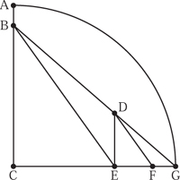
Figure 4.3. A geometric construction of .

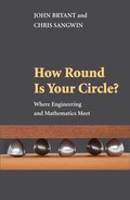
Before we do this, we digress and describe here an old Chinese method for constructing a line units long (a good approximation to π), as given by Gardner (1966). It is worth mentioning as an example of a Euclidean construction, and also to show how a fraction with the awkward looking denominator 113 can be drawn using only Euclidean means. Start with a quadrant ACG of unit radius, as shown in figure 4.3, with AB = AC and join B and G. With DG measuring half a unit in length, drop a perpendicular to meet CG at E and now draw DF parallel to BE. FG is then units long.

The proof that FG = this assertion relies on the Pythagorean theorem as well as the properties of similar triangles, so we begin by noticing that

BG² = CG² + BC² = 1 + ².

Hence BG = . By the properties of similar triangles,

and

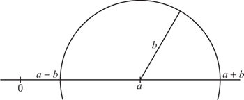
Figure 4.4. Constructing a ± b.

CE = 1 − EG and EF/DE = CE/BC, from this we have

and hence FG = as claimed. We actually wanted to construct but originally. To complete the construction, the unit radius is stepped off three times with the compasses to bring the length to .

4.3 Building the World’s First Ruler

We shall be a little more systematic in this section and we shall consider exactly which points we can mark on our ruler, and decide how to do this. We say that we can construct the number if we can construct the point on the ruler which is that length from the origin. What we shall show is that given any two previously constructed lengths a and b we may construct a ± b, a × b and, provided that b ≠ 0, a ÷ b.

From the previously constructed integers this allows us to construct all the rational numbers. But it also gives us a lot more, since every time we construct a new number, we can in a sense complete the number system by incorporating this with the existing collection of numbers using the same operations.

So to work. Constructing a ± b is very straightforward using the construction shown in figure 4.4. Simply open the compasses to a radius of b and draw a circle with centre a. The circle will intersect the line at the points a + b and a − b. It really is as simple as that.

Figure 4.5. Constructing a × b.

To construct a × b, or more simply ab, from the two lengths a and b we draw a line and mark the positions of 0, 1, a and b as shown in figure 4.5. Note that the diagram illustrates the case 0 < b < 1 < a, although this is unimportant. Mark any other line through 0, called l₀, and draw a circular arc with centre 0 and radius b. Where this arc intersects l₀, mark on the point B. Connect B and 1 with a straight line l₁. Mark the line, l₂ say, perpendicular to this through 1. Mark another line, this time l₃, through a and perpendicular to l₂. Where this intersects l₀ we mark the point A. If we choose we can mark the length 0A on the original line with a circular arc. In any case, the length 0A is indeed the required length a×b. This may be seen since the two triangles aA0 and 1B0 are similar, so that

That is to say, 0A = ab.

To construct a÷b we refer to figure 4.6 and draw a straight line upon which we mark 0, 1, a and b. Again, we draw an arbitrary line l₀ through 0. Next, draw the circular arc through 0 of radius 1 and label the intersection of this arc with l₀ as B. Connect B to the point b. This line is l₁, and from this drop the perpendicular through a. Draw a further perpendicular to this new line through a and where this crosses l₀ we mark a point A. By drawing a circular arc back onto the baseline we have constructed the length a ÷ b. To see this we notice that the two triangles 0aA and 0bB are similar. Therefore,

Figure 4.6. Constructing a ÷ b.

and therefore 0A = a ÷ b.

Armed with the four arithmetic operations (addition, subtraction, multiplication and division) together with the two numbers 0 and 1 we may construct any rational number m/n, where m is an integer and n is any non-zero integer. Thus all rational lengths are possible. If you are not familiar with rational numbers, look ahead to chapter 9.

4.4 Ruler Markings

In section 9.1 we show that there are other lengths that are not rational numbers. An example is , although this length is easy to construct using a ruler and compass since we just take the diagonal of a unit square.

Hence, we may construct considerably more than just rational numbers m/n. In particular, given any positive length a we may construct as follows. With reference to figure 4.7 construct the lengths 0, a, a + 1 and (a + 1) using the above constructions. Now draw the circle centred at (a + 1) of radius (a + 1). Draw a line through a perpendicular to the baseline and mark where this line intersects the circle, by A say. We are interested in the distance from A to a, which we call x. By theorem 1.1, the triangle through 0, A and a + 1 has a right angle at A. Therefore the two smaller triangles in figure 4.7 are similar. Using similarity we have

Figure 4.7. Constructing .

so that x² = a, from which we have x = .

So we can now add a mark for on our ruler if there is already a mark for a. What else is possible? Can we mark What about π? In fact, can we mark any point we can think of, and if not can we decide exactly which numbers are constructible?

To answer this last question we now think of coordinates of points in the plane, rather than restricting our attention to our straight-line ruler. Given a point P_i, we think of this as having coordinates (x_i,y_i). So, for example, if the first two points we construct mark out our unit length on a horizontal line we think of these as having coordinates (0,0) and (1,0). Our straight edge and compass constructions allow us to generate points only from the intersections of

1. two lines,
2. a line and a circle,
3. two circles.

What we consider next is how to describe these possibilities using algebra.

First, assume we have two points P₁ and P₂ with coordinates (x₁,y₁) and (x₂,y₂). Take another arbitrary point on the line connecting these, and call this (x,y) (see figure 4.8). By similar triangles,

Figure 4.8. Points on a straight line.

Rearranging this gives

Since x₁, x₂, y₁ and y₂ are constant we can express this as

ax + by = p,

which is one form of the equation of a straight line.

Let us take four points P₁,...,P₄ with coordinates (x_i,y_i). The intersection of the lines through P₁, P₂ and P₃, P₄ will be given by any solutions (x, y) to the simultaneous equations

x(y₁ − y₂) + y(x₂ − x₁) = x₂y₁ − x₁y₂,

x(y₃ − y₄) + y(x₄ − x₃) = x₄y₃ − x₃y₄.

Now, a solution may not exist (and indeed does not if the lines are parallel), but if a solution does exist finding it requires only the use of the mathematical operations of addition, subtraction, multiplication and division.

Next take a circle of radius r centred at P₃ (with coordinates (x₃,y₃)). The Pythagorean theorem tells us that points on the circle with coordinates (x, y) must satisfy the relationship When this circle and a line through P₁, P₂ meet, we have simultaneous equations:

(x − x₃)² + (y − y ₃)² = r².

x(y₁ − y₂) + y(x₂ − x₁) = x₂y₁ − x₁y₂,

(x − x₃)² + (y − y₃)² = r².

Again, there is no reason to suppose that the line and the circle do intersect. If they do, the coordinates x and y are related using only the operations of addition, subtraction, multiplication and division along with the extraction of square roots.

The case of the intersection of two circles is similar. The only mathematical operations needed to generate the coordinates are addition, subtraction, multiplication, division and the extraction of square roots. What we have done is turn a geometrical construction of lines and points into an algebraic discussion of what operations one is allowed to use to construct our numbers. The above discussion points the way to the following theorem, which characterizes precisely which numbers are constructible.

Theorem 4.1. A number is constructible if and only if it may be obtained from the integers by repeated use of addition, subtraction, multiplication, division and the extraction of square roots.

Proof. If a may be obtained from the integers by repeated use of addition, subtraction, multiplication, division and the extraction of square roots, then the above constructions show how we may construct the number with a straight edge and compass.

Conversely, let us assume that a number a is constructible. This means that there is a finite sequence of simple ruler and compass constructions from (0,0) and (1,0) that generate points P₁ and P₂, the distance between which is the length a. Each point generated in the construction occurs only at the intersection of two lines: a line and circle or two circles. From the discussion immediately preceding the theorem, we can see that the coordinates of such points can be obtained from previous coordinates using only addition, subtraction, multiplication, division and the extraction of square roots. Since we have a finite sequence of such points starting from (0,0) and (1,0), the coordinates of P₁,P₂ are obtained from the integers by repeated use of these operations. Since

it follows that a can be obtained using only addition, subtraction, multiplication, division and the extraction of square roots.

Although the above is only a sketch of the proof of the converse, a more rigorous discussion can be found in, for example, Stewart (1989, theorem 5.2). What theorem 4.1 tells us is that many lengths are impossible to construct using only a straight edge and compass. However, given a number a it may not be easy to tell whether it can be expressed using the above operations. In fact, whether a is constructible depends on whether it occurs as the root of certain polynomials with rational coefficients. For example, the square root of a occurs as the root of the equation x² − a = 0. If a number a satisfies one such polynomial then it will satisfy many. What is important is the smallest degree of such a polynomial. It turns out that a is constructible if and only if the degree of the smallest polynomial is a power of 2, i.e. 2ⁿ.

The cube root of 2, that is , is not constructible since it satisfies the equation x³ − 2 = 0 but no polynomial equation with rational coefficients of degree 1 or 2. This allows us to solve the following classical problem. Given a cube, with unit sides, is it possible to construct a cube with twice the volume? In order to do this we need to construct the length . The fact that is not constructible shows that it is impossible to ‘duplicate the cube’.

Numbers which do not occur as the root of any rational polynomial equation are known as transcendental. To conclude that π cannot be constructed using straight edge and compass we need to know that π cannot be constructed using the additional operation of taking square roots. In fact, the number π does not satisfy any rational polynomial and so cannot be constructible. The proof that π is transcendental is too long to repeat here, but can be found in, for example, Stewart (1989, chapter 6). Another example of a transcendental number is the base of the natural logarithms, e, which we shall encounter in chapter 8. Hence it is also impossible to construct this number.

The impossibility of constructing π solves the second classical problem, that of ‘squaring the circle’. Given a circle of radius r, can we construct a square with the same area? Since the area of the circle is πr², we need to construct the length . This is possible if and only if we can construct π. Since we cannot do this we may not square the circle.

These well-known impossibility proofs are encountered as part of most university undergraduate mathematics degrees. However, there are still those who seek in vain a geometrical construction that will square the circle, duplicate the cube or trisect the angle. Such people sometimes have a good grasp of geometry, and certainly great tenacity. Unfortunately, these attempts are bound to be futile, and the resulting lengthy calculations must inevitably contain at least one error. Professional mathematicians, including the authors, still occasionally receive unsolicited proofs of the impossible. The most recent bundle of papers one of us received arrived by airmail and included a ‘proof’, using exactly the ruler and compass constructions above, that

Anyone with a pocket calculator can immediately see that

π ≈ 3.141 5926... ≠ 3.146 4466...,

which should be enough to suggest strongly that something is amiss. So what should the professional do? Clearly there is not sufficient time to wade through pages of nonsense, carefully correcting the inevitable mistakes. Since we know these constructions have been proved to be impossible, we know without reading the argument that it must be flawed. One option is to ignore such mail, but this may also be a serious error since G. H. Hardy discovered one of the greatest mathematicians, S. Ramanujan, on the strength of an unsolicited bundle of papers and helped obtain for him a fellowship at Cambridge. This is a famous story, told by Hardy in his A Mathematician’s Apology (Hardy 1967). Furthermore, to ignore such correspondence confirms any suspicion the authors may have that the professional mathematical establishment is in conspiracy against them. Often this strengthens the resolve of the author who eventually publishes privately, as a newspaper advertisement or even, if the calculations are sufficiently extensive (unfortunately, to them at least, a synonym for ‘important’), as a book. When such work is combined with a religious conviction, the result can be far from nourishing to the soul, as anyone who has tried to read such works as MacHuis-dean (1937) can attest.

4.5 Reading Scales Accurately

While this chapter is mostly concerned with the problem of marking out scales accurately, an equally important problem is that of actually reading the scales themselves. Of course, a magnifying glass or microscope is invaluable here, and this is exactly what was used for precision work with standard lengths. However, there are also techniques which allow an extra decimal place of accuracy to be read directly with the naked eye. For example, while it is possible to read a normal rule to the nearest millimetre with the naked eye, there is no way to read a scale to one-tenth of a millimetre directly. Furthermore, marking a scale with ten marks in every millimetre would result in too many lines. The scale would be cluttered and the individual lines would become confused. However, the situation is not hopeless, and it is possible to design a scale capable of providing this extra place of accuracy. Indeed, the most common solution is known as a Vernier scale.

Vernier scales are ingenious and simple and they are now present on almost all analogue devices from callipers, which measure length, to surveying instruments, which measure angles, to planimeters, and so on. They were invented by Pierre Vernier (1584–1638) and described in his book, La Construction, l’Usage et les Propriétés du Quadrant Nouveau de Mathématique (‘The New Mathematical Quadrant’) in Brussels in 1631. A quadrant is used to measure angles, and as the name implies it is a quarter of a whole circle. As with so many other inventions that are discussed in this book, it languished almost unknown for many years after its original invention. For example, very few of the instruments in Bion’s catalogue Traité de la Construction et des Principeaux Usages des Instruments de Mathématique (1709) (translated into English as Stone (1753)) contain a Vernier scale. We shall return to these in more detail in chapter 5.

Figure 4.9. A Vernier scale.

Here, we shall describe a linear Vernier scale, rather than the original angular device, but the principles are the same. Imagine an equally spaced scale together with a pointer which provides a reading on an instrument. In our case this is a reading of length (see figure 4.9(a)). The pointer is just to the right of 1.6, so let us call this reading 1.6 + x. Since the pointer does not line up with one of the scale markings, it is necessary to estimate the value of x. The Vernier scale is a method which reduces the amount of guesswork in this estimation, and consists of another scale which supplements this pointer. However, the Vernier scale is spaced at intervals of 0.09, not 0.1 as is the original scale in figure 4.9(a): see figure 4.9(b). To use this, count along to find the line on the Vernier scale which matches up most closely with a line on the top scale. In the figure above, this is the second line along the Vernier scale. Now, since the Vernier scale is spaced at intervals of 0.09 and the top scale is at 0.1 we have to solve the equation

x + 2 × 0.09 = 2 × 0.1,

obviously giving x = 0.02. Hence, the pointer is at position 1.62 on the top scale. In practice, you just count along the Vernier until the two scales coincide. Then you know the extra decimal place, without having to estimate or perform the above calculation. Hence, the Vernier scale is an ingenious, simple and accurate mechanism.

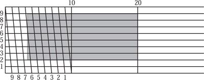
Figure 4.10. Obtaining extra accuracy with diagonal lines.

There is another common mechanism which is often found on rulers that can be used to gain an extra place of accuracy. For the purposes of illustration, we shall assume that we have a ruler with equal graduations one unit apart. Upon this draw ten lines parallel with the edge of the ruler and one unit apart, with one unit separating them. Next draw diagonal lines as shown in figure 4.10. These diagonals intersect adjacent parallels one-tenth of a unit apart. Of course, these diagonals need only be drawn in one 10 × 10 unit square to use the whole length of the ruler.

Imagine you need to use this device to measure the length of something, such as the grey rectangle shown in figure 4.10. First estimate the length to the nearest 10 units or so, in our case between 10 and 20 units. Rather than placing one end of the object to be measured at the zero of the scale as one usually does, place it so that one end is on the 20 unit line and the other end falls in the diagonally separated grid. Move the object up and down until it lines up perfectly with a diagonal. This will now allow a one-tenth of a unit length measurement to be read off. In our case, the grey rectangle is 16.7 units long. In practice these scales are rather hard to read. They are also very difficult to make and rely on being able to draw, originally by hand and eye, very accurate diagonals. For a more accurate measurement of length, callipers with a Vernier scale are much better, although correspondingly more expensive to produce, than a printed scale. Cutting along the horizontal lines for 0 and 10 and rolling the paper round so that these lines coincide gives us a screw thread. Such a screw forms the basis of micrometers and the fine adjustment mechanisms used in instruments of all kinds.

4.6 Similar Triangles and the Sector

Another important topic is that of similar triangles: two triangles are similar when the sets of angles are equal. When this happens, the lengths of corresponding sides are related by a fixed multiplication factor. Hence, similarity really has a lot to say about scale.

One classical mathematical instrument which is based on the properties of similar triangles is the sector, which is an instrument consisting of two rulers of equal length that are joined by a hinge. A number of scales are drawn on the instrument facilitating various mathematical and trigonometrical calculations—an example is shown in figure 4.11. This sector, approximately 12 in long, is made from ivory and brass. In common with many devices in this book, the issue of who first invented the sector is not without controversy. Its invention is often attributed to Galileo Galilei (1564–1642) in approximately 1597 (see, for example, Meskens 1997; Smith et al. 1996). However, Hopp (1998) claims that the sector was invented by a Guidobaldo de Monte, who was a friend of Galileo, as early as 1568. It turns out that the first scientific instrument to contain a logarithmic scale was the sector, not the slide rule. This was an innovation of Edmund Gunter, and its history is explained in section 11.2.

The sector can be used to perform many different numerical and plane or spherical trigonometrical calculations. The remainder of this section is a basic introduction to some of the calculations that are possible using a sector and an explanation of the most commonly appearing scales. There are two principal modes of operation: fully open as a straight rule, or partially open with the scales radiating out from the centre. At all times the sector is used in conjunction with a pair of compasses or dividers.

Figure 4.11. A sector.

When open fully, the long outside edge is marked with a scale divided into ten equal parts, each of these are further subdivided into ten parts. This scale is known as the scale of decimals. On one flat side close to the outside edge of the sector is a scale of inches. Typically a small pocket sector will be 12 in long when opened out. (If you ever have access to an old ivory sector, you might check to see how much shrinkage has occurred over the years.) On the other side are probably three long scales parallel to the long outside edge of the sector. These are marked N, S and T. The line N is a ‘Gunter line’, that is to say, a line marked in a logarithmic scale. The other two lines, S and T, are the lines of sines and tangents, respectively. These three scales are usually referred to as the lines of artificial numbers. The Gunter line, or logarithmic scale, is dealt with in chapter 11.

The other scales radiate out from the point where the two rules are hinged and are used with the sector open at an angle. Many of these scales are inscribed twice, once on each leg of the sector, and are referred to as double scales. These will be described individually in more detail below. When the compasses are used on a scale to measure a length from the centre it is called a lateral distance: distance x in figure 4.12, for example. When a measure is taken from any point on the line to its corresponding point on the line of the same denomination on the other leg, it is called a transverse distance: the distance y in figure 4.12, for example.

The sector derives its name from Euclid’s Elements (book VI, proposition 4), which states that similar triangles have their like sides in proportion. To see why this theorem forms the mathematical basis of the sector, consider the two similar triangles shown in figure 4.12. We assume that the large outer triangle OMN has a small similar triangle OPQ within it. The line PQ is parallel to MN. The proposition can be used to deduce that a/b = x/y. The sector uses exactly this principle when the arms are open at an angle.

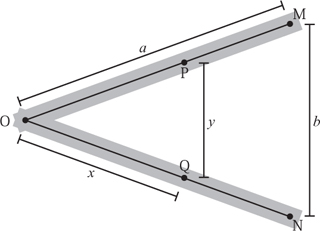
Figure 4.12. The principle of a sector.

Multiplication can also be performed with the arms of the sector open. Locate the scales marked L which radiate along the arms from the centre and are marked in ten equal parts. Numbers can be multiplied using these scales by recalling figure 4.12, where the lines OM and ON represent the scales marked L on the legs of the sector and O is the point at which the legs pivot. Recall that a/b = x/y or ay = bx. The length OM is always fixed at 10 units. We are left with three unknowns, x, y and b. Take a pair of compasses open to a distance which represent a length b. Using the compasses as a guide, open the sector so that the distance between M and N is the length b. Next locate the points P and Q that are a lateral distance x along the scale. Using the compasses take the transverse length y. This length can be read by placing one point at O and the other point on the line OM and reading directly on the evenly spaced scale. The length y that has been constructed is the answer to 10y = bx. Division can be performed by an obvious reverse process.

For multiplying numbers this process is slow, requires a high degree of manual dexterity and is not very accurate. However, it is much quicker than the geometric construction given in section 4.3. So, for a quick approximate and geometric calculation it does have limited practical use. Perhaps the main use would be during a plane figure construction where it is necessary to construct a line of a given proportion from one already on the figure. This clearly removes the need to measure lengths and multiply numbers. This shows that multiplication of lengths can take place in an entirely graphical way. To understand the difficulties it is really worthwhile constructing a simple sector, or drawing a sector at a fixed angle and marking on the two scales.

Measuring Plane Angles

The sector can also be used to construct angles using the lines of chords. This is a double scale, marked C, with scales that run from 0 to 60. To protract an angle of 0 < t < 60° use the scale C and open the sector so that the transverse distance MN equals the lateral distance OM = ON. It is clear that the angle MON = 60°. Using the compasses on the scale measure the lateral distance from O to t. Draw a circular arc, centred at O, from M to N and place one point of the compass at N. Where the other point intersects the arc will be marked R. The angle RON is t. Angles can be measured using the reverse procedure. An angle s greater than 60° can be protracted by repeatedly subtracting 60° or 90° from s.

Inscribing Polygons Inside a Given Circle

The typical sector also came with scales that could be used to easily inscribe a regular polygon inside a circle of any given radius using the line of polygons. This double scale, marked POL, usually on the inside of the sector, is marked from 12 nearest O down in unit steps to 4 at N and M, and these numbers refer to the number of sides on the polygon itself. Hence, the sector could be used to draw polygons with seven, nine or eleven sides, which the classical theory shows is impossible using only a straight edge and compass.

Refer again to figure 4.12, this time assuming that ON represents the scale POL. Draw the circle in which you wish to inscribe the polygon and keep the compasses open at the radius. Remember that the length of the sides of an inscribed hexagon is the radius of a circle. So, use the compasses to open the sector so that the transverse distance between the 6s on the POL scale equals the radius of the circle you have just drawn. The transverse distance between the figures is the lengths of the sides for an inscribed polygon with that number of sides. For example, to inscribe a square measure the transverse distance between the 4s on the POL scale and use this to walk the compasses round the circle. Then inscribe the polygon directly using these points.

It is also straightforward to construct a polygon with a given number of sides and a given side length, as opposed to an inscribed polygon. To do this, measure the length of the sides, y, with the compasses. Let P and Q be points on the POL scale corresponding to the number of sides of the proposed polygon. Open the sector so that P and Q are a distance y apart. The radius of the required circle is the transverse distance between the 6s. This is simply the reverse process although here the sector may not open wide enough.

Other Scales

The above gives some examples of the range and types of calculations that can be performed by the sector. The other scales can be used for a variety of other calculations, including spherical trigonometry, that are not discussed in detail here. A full description of how to use such a sector can be found in, for example, Heather (1871).

The sector was a standard component in a set of mathematical instruments. However, the smaller pocket sectors would have been of little or no use because of the difficulty in using them accurately. Compass points damage scales with regular use and this reduces the accuracy of the instrument. The large number of well-preserved sectors that exist would add weight to the school of thought that claims they were of little practical use, other than for school geometry problems. However, large instruments were used by artillery officers for calculations in the field.