Chapter 5

DIVIDING THE CIRCLE

Devyde it into sixty parties equals.

Chaucer (1872)

 

 

Length is a measure of the extent of a one-dimensional line. In defining length in chapter 4 we had considerable freedom in taking an arbitrary unit length. It was then a geometric task to divide this into fractions and to build the world’s first ruler.

In this chapter we measure the extent of rotation, and here we have a natural base unit of one complete rotation. The choice now is how to divide the circle. The quotation from Geoffrey Chaucer (1343–1400) above, from the first scientific book published in England in the vernacular rather than in Latin, describes dividing angles on the astrolabe. An astrolabe is a device with which astronomical measurements can be taken, and it is no coincidence that astronomers were, as a profession, most interested in accurate angular measurement. Of course, navigation is closely related to astronomy and hence finding one’s position using a sextant also relies on accurate measurement of angles. Surveying and cartography also depend on being able to triangulate one’s position. Keay (2000) gives a very good idea of the care and precautions taken to set up the datum line 7 miles (12 km) long as the basis for the meridian survey of India in the nineteenth century. From the measured angles and a datum line of known length the mathematical task is to reconstruct the ground surveyed. All this relies on accurate measurements.

All of these applications are only possible if accurate instruments are available with which to undertake the measurements. Progress in science goes hand in hand with progress in the development of accurate and reliable instruments, although in the history of science the importance of instrumentation is not always given its due weight. As Chapman (1990) succinctly puts it:

Instruments came to be seen not only as refinements or aids to human perception, but as the very arbiters in scientific discussion, when the acceptance or otherwise of a theory depended upon the interpretation of observational evidence.

The invention of the telescope by Galileo Galilei opened up new worlds to science. The use of the telescope as an observational tool is usually given prominence, for example to view the moons of Jupiter. Certainly less immediately glamorous are its uses for measurement, but it is this which really drove science forward.

Before the invention of the telescope, astronomers such as Tycho Brahe (1546–1601) relied on naked eye measurements. Essentially there are two problems in astronomy. The first is in observing the object in the sky, and lining up an instrument upon it. The second is in recording the position of the instrument, for example by reading the angular position. Originally it was sufficient to use cross-hairs, since the accuracy of the whole process was determined by the accuracy of the angular scales. Gradually the design of such scales was improved so that greater accuracy could be achieved. For example, the system of diagonal lines illustrated in section 4.5 was applied to instruments such as the octant shown in figure 5.1. Such improvements in scale design meant that the astronomer’s overall accuracy was hampered by his ability to see an object in the sky and line up the measuring device to take a reading.

Experiments by Robert Hooke (1635–1703), repeated in more recent studies, showed that the naked eye could resolve an object that occupies about 1′ (one minute) of arc. Kepler, for example, was concerned with a difference of 8′ between the position of a planet predicted by a circular orbit and what was actually observed. It was only with Tycho Brahe, the last and greatest naked eye astronomer, that orders of accuracy approaching 1′ total error were achieved. Hence, the level of accuracy that the naked eye can achieve is simply not sufficient for testing astronomical theory.

Figure 5.1. An eighteenth-century octant from Stone (1753).

It is the Yorkshire mathematician William Gascoigne (1612–44) who is credited with putting cross-hairs into a telescope to create a telescopic sight. The key to this is to place the cross-hairs inside the telescope at the instrument’s common focus. Gascoigne was observing the Sun when he noticed that a spider had spun a web inside the telescope. By chance this was in sharp focus, and from this discovery Gascoigne developed a practical telescopic sight. The practical use of this was obvious to him and his friends, and it is reported in Derham (1717, p. 604) that when the astronomer John Horrox first saw the invention it ‘ravished his mind quite from itself and left him in an extasie between admiration and amazement’.

Lenses were also applied to read scales more accurately, and the astronomer Ole Römer (1644–1710) used a low-power microscope containing a number of hairlines to remove the problems of two scales wearing against each other. Gascoigne also developed a device consisting of two movable cross-hairs, controlled by a graduated screw. By measuring the number of turns, the distance between the two cross-hairs could be calculated and from this the angle between two objects which were very close together could be calculated. This was used by him to measure the angular width of the Moon and the planets. Of course, the accuracy of this device depends crucially on the accuracy of the threads of the screws, which in the early seventeenth century were extremely difficult and expensive to make by hand. Screw threads were also used to move and position telescopic sights accurately, although early designs by Robert Hooke and others were not particularly successful from a practical point of view. The Astronomer Royal John Flamsteed (1646–1719) complained bitterly that he was ‘much troubled with Mr Hooke who, not being troubled with the use of any instrument, will needs force his ill-contrived devices on us’ (Flamsteed 1725, p. 103).

5.1 Units of Angular Measurement

It is well worth pausing for a moment to review mathematical systems for angular measurement. The most commonly used system for measuring angles is the division of a circle into three hundred and sixty degrees, i.e. 360°. Each degree is subsequently divided into sixty minutes and each minute into sixty seconds. An angle is then written as 17° 34′ 12″. Each minute is ≈ 0.0167 of a degree, and each second is ≈ 0.000 278 of a degree. As we have seen, dividing a circle into six equal parts is simple, and can be done accurately. Then subdividing each into sixty equal parts to give degrees and then again into minutes and seconds is a remnant of the ancient Babylonian base-sixty number system. This division into 360° is also convenient from a practical point of view. For example, on a basic school protractor with a diameter of 90 mm a single degree occupies an arc length of about 0.75 mm on the edge. This is perfectly easy to distinguish by eye, and yet still small enough a unit to be practically useful. Since 60 and 360 have so many integer factors, many fractions of a rotation are easy to express exactly as whole numbers of degrees.

Mathematicians use a different system for measuring angles and it is known as the radian. In this system a circle is divided into 2π radians. The advantage of this is that many formulae become extremely simple and elegant to express. For example, in a circle of radius r take an arc with angle t, measured in radians. The arc length is simply rt. The corresponding formula, with t in degrees, is πrt. However, since π is an irrational number there is no longer a whole number of radians in a whole number of full rotations. From a practical point of view this is a catastrophe.

Another unit for measuring angles is the decimal degree. In this scheme a right angle is divided into 100 units, and many modern scientific calculators implement these units as grads. For military purposes the artillery divide a full circle into 6400 parts, called mils, not to be confused with the spoken abbreviation for a millimetre.

It is clear that astronomical tables of angles were not used solely by their original observer but were intended for publication for the benefit of other astronomers and navigators. In these circumstances it is vital that there should be a widely understood and accepted unit of angle, and we naturally base our protractor on a circle of 360°.

We shall see in section 5.4 that, from the practical point of view when trying to engrave a graduated scale using only geometric constructions, 90° in a quarter of a rotation is not as convenient as the number of factors would first suggest. In particular, it is always possible to divide any angle exactly into two equal parts, but it is in general impossible to divide an arbitrary angle into three. Furthermore, we know that 60° can easily be marked to a high degree of accuracy, using the radius of the circle. From this, 30° and 15° can be found by simply bisecting repeatedly. To go any further we need to divide by three and then five, which poses a problem.

Instead, George Graham (1675–1752) chose to divide a right angle into 96 equal units. In this, the radius will strike off 64 units of angle, and since this is a power of two the remainder can be repeatedly halved to get single angular units. He used this scheme on an 8 foot quadrant in the Royal Observatory in Greenwich. This was engraved with both a 90° scale and an adjacent scale of 96 units. These two scales allowed a cross-check, and the whole construction was carried out with such skill that the two arcs differ by no more than 6″, which is approximately 0.0017°. The sketch of this quadrant given in Stone (1753) is reproduced in figure 5.2.

Figure 5.2. A mural quadrant from the Royal Observatory in Greenwich.

While the 96 point scale is an elegant solution to the problem of geometrical construction, it is somewhat unsatisfactory. Users want accurate scales based upon the familiar 90°. It is awkward, and a potential source of error, to convert between the two systems. It was John Bird (1709–76) who solved this problem, and he was also one of the first practitioners to leave a detailed account of his own methods of working: Bird (1767), which was written for the Board of Longitude. He developed a system based upon 85° 20′ and to see why this works we note that 85 × 60 + 20 = 2¹⁰ × 5. Hence, by repeatedly dividing the angle 85° 20′ in half we eventually arrive at an angle of 5′. It only remains to construct the crucial angle of 85° 20′ sufficiently accurately. He did this by accurately constructing 30°, 15°, 10° 20′ and 4° and adding them together. In particular, he drew a large circle and calculated and measured the lengths of the chords subtending some of these angles, measuring them to th of an inch. This introduced the possibility of error, and it is a testament to his professional skill that such a method could actually be made to work. A large number of independent cross-checks were then undertaken to gauge the accuracy of this one angle, before the division of this angle into halves to create a scale of degrees. According to Ludlam (1786), this technique was a great success, both in the Greenwich observatory and in Bird’s many other instruments.

When working at this level of accuracy the temperature of the workplace matters. If the metal being engraved and the compasses are made of different materials, then not only must they be at the same temperature but also at a well-defined temperature. Otherwise, problems will arise with differential expansion. In metrology, 20°C is now taken to be a standard working temperature.

After the 1780s astronomy moved away from large fixed quadrants to the use of full graduated circles. Whereas the division of the quadrant is essentially a geometrical exercise, dividing the circle is mechanical, and so we do not pursue the practical problems of astronomy further. Rather, we consider the geometry and eventually show how to trisect an angle by other means, something which practitioners such as Bird had assiduously avoided doing.

While this chapter concentrates on the mathematical problem of dividing the circle, the preceding discussion gives some background to the associated practical problems with constructing an astronomical instrument, which is very much more than an accurate protractor.

5.2 Constructing Base Angles via Polygons

It would be tempting for our application to mark out the smallest angle to a supremely high degree of accuracy and use this to mark out all others by walking the protractor around the circle.

This would result in a accumulation of errors. Instead we work from the other direction or dividing larger angles into parts. We first note that there is a strong connection between angles and regular polygons. We notice immediately that if we can construct an n-sided regular polygon, we can construct an angle of 360°/n. Conversely, if we can (somehow) construct an angle of 360°/n, then we can construct an n-sided regular polygon inside a circle. So, at least to begin with, we concentrate on building regular polygons.

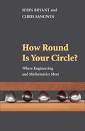
It is straightforward to construct shapes such as equilateral triangles, squares and regular hexagons. For the hexagon, for example, start by drawing a circle and mark some starting point A₀ on this (see figure 5.3). Keeping the compass radius fixed, draw a second circle centred at A₀. Where this intersects the original circle mark A₁ and A₅. Next draw a circle centred at A₁. This will intersect the original circle at A₀, but also at a new point A₂. Repeat the process centring a circle at A₂ to generate A₃. This is similar to walking around the circle with the compasses to mark out successive points. In fact, one does not need to draw the entire circle at each stage and only small arcs have been included in figure 5.3 to keep the diagram uncluttered. Walking around a circle with a pair of compasses in this way is exactly how we will construct regular polygons in general. We only need to construct the length of one edge and the circle in which the polygon is to be inscribed.

Let us refer to an n-sided regular polygon simply as an n-gon for brevity. Assuming we can construct an n-gon, then we can certainly construct a 2n-gon, a 4n-gon, etc., by halving angles. Similarly, if n is not prime, say n = pq where p and q are integers, we can also easily construct a p-gon by simply skipping every q vertices. For example, to construct a 3-gon (better known as an equilateral triangle) from a regular hexagon, miss out every other vertex. From this observation we see that it will be important to consider the ‘prime-gons’. The following theorem shows exactly which n-gons are constructible using only a straight edge and compass, but the proof is not included.

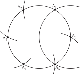
Figure 5.3. Constructing a regular hexagon.

Theorem 5.1. An n-gon is constructible using straight edge and compass if and only if

n = 2 ^kf₁ × · · · × f_m,

where the f_j are different Fermat prime numbers. That is to say, f_j are prime numbers of the form 2^2j + 1 for some j = 0,1,....

To properly understand how restrictive this theorem is, let us consider which numbers of the form 2^2j + 1 are prime. The sequence is

 

j	22j + 1
0	3
1	5
2	17
3	257
4	65 537
5	4 294 967 297

This sequence looks promising, since 3, 5, 17, 257 and 65 537 are all prime. However, 4 294 967 297 = 641 × 6 700 417, so it is not prime. Indeed, so far no other primes of the form 2^2j + 1 are known, and whether there are any or not is an open problem. So, currently there are only five choices for the f_j in theorem 5.1, although we can take any combination of these or none at all. This is really quite limiting because by telling us which n-gons are constructible, the theorem tells us which basic angles, or rather fractions of a circle, are not constructible.

Figure 5.4. Constructing a regular pentagon.

Hence, we have a very limited range of base angles from which to build our protractor. From a practical point of view, adding angles is not a sensible strategy, since errors are cumulative. More importantly, there is no way of obtaining an independent check of the scale. Hence, for our application the most important task is to divide angles. Once all angles have been marked out they can be checked against each other.

5.3 Constructing a Regular Pentagon

To illustrate this excursion into polygons we shall explain the construction of a regular pentagon, shown in figure 5.4. Let us take a quadrant AOB in a unit circle, i.e. OA = 1 and the angle AOB is 90°. Mark C as the midpoint of the radius, then by the Pythagorean theorem

With C as the centre draw an arc of radius AC to cut the diameter OB at D, so that

As a complete digression you will notice that OD/OB is the Golden Ratio. Using the Pythagorean theorem again,

The final step is to draw an arc of this radius from A cutting the circle at E and F. Triangle OEA is isosceles and so we can write

giving t = 72°. AE and AF are therefore the sides of a regular pentagon.

Although it is not a Euclidean construction, we should mention that one very neat alternative way to construct a regular pentagon for yourself is to take a strip of paper with parallel sides and tie a normal overhand knot. Carefully tightening and flattening this knot leaves a regular pentagon. Constructing a seventeen-sided shape is actually quite a complicated straight edge and compass construction, and one shudders to imagine trying to construct the 257- and 65 537-sided figures in practice. Indeed, even though a polygon of 65 537 sides is of no help to us in constructing a protractor, do not be tempted to try it out of general interest.

A too-persistent research student drove his supervisor to say ‘Go away and work out the construction for a regular polygon of 65 537 (= 2¹⁶ + 1) sides’. The student returned 20 years later with a construction (deposited in the archives at Göttingen).

Littlewood (1986)

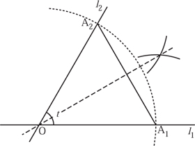
Figure 5.5. Dividing the angle t in half.

5.4 Building the World’s First Protractor

The object of this section is to discover how far it is possible to graduate a protractor, such as a typical school protractor, into units of one degree using only exact Euclidean constructions involving a straight edge and compass.

The symmetry of a circle is such that we can confine our description to constructing a quadrant, and this can easily be constructed by starting from a straight line: an angle of 180°. Taking a vertex wherever we please on the line, the next constructional step is to bisect this angle to obtain an angle of 90°. This can be done by constructing a perpendicular to the line, just as in figure 4.2.

We have claimed that it is possible to divide an arbitrary angle into two equal parts. To show how, we begin with an angle t between two previously constructed lines l₁ and l₂, which meet at O. Such a configuration is shown in figure 5.5. To divide this angle in half draw a circle centred at O and where this meets l1 and l₂ mark A₁ and A₂. Connect these with a straight line, l3. As detailed above, construct the perpendicular to l₃ through O, shown in figure 5.5 as the dashed line. That this line divides the angle t in half is easily proved using similar triangles. This procedure is known as bisecting an angle.

The prime factors of 90 are 2, 3, 3 and 5, so we can bisect 90° to reach 45°. No further bisection is possible because we do not wish to introduce fractions of a degree into our quadrant. This leaves us with the factors 3, 3 and 5 and it is impossible to trisect an arbitrary angle using only Euclidean tools, so we must find some alternative method. Since we are interested only in exact trisection, which is generally impossible, we defer discussion of approximate and mechanical methods to a later section.

We can, though, construct an angle of 60° by the familiar technique used to define the vertices of an equilateral triangle and so we have effectively trisected 90°, proving that it is possible to trisect some angles. 60° has two factors of 2 so that we end up with graduations at 15° intervals. This is an opportunity to check the precision of our work: 45° was first constructed by bisecting 90° and we have now produced the same angle independently by twice bisecting 60°. We are not making a large astronomical quadrant and so we do not really need this check, but on any precision instrument any way of verifying our work as it progresses is very welcome.

We can use part of the regular pentagon, giving angles of 72° and 18° to add to our quadrant. 72 has prime factors 2, 2, 2, 3 and 3 so we can now add angles at 9° intervals. Furthermore, since the difference between 72° and 60° is 12°, we find that some 3° graduations are possible after further bisections.

In principle, but maybe not in practice, we could repeat the constructions based on 60° and 72° on two of the angles we have already marked on the quadrant. The result, after some bisections, is a full scale of divisions 3° apart. Whatever we do though we cannot further divide 3° into units of 1° so we must resort to approximate methods.

There is, however, another set of practical problems associated with the width of the lines. Harking back to chapter 1, in all instruments we are relying on the intersection of two lines of finite width to define points through which a radial line must pass, or to form centres for further constructions. To put this into an everyday context, the interval between 1° graduations is about 0.75 mm on the circumference of a typical school protractor. A commonly used drawing instrument is a pencil with a 0.5 mm diameter lead.

As a general rule for locating a point, it is always best if the two intersecting lines cross at right angles, as its centre is most sharply defined when the overlap is square rather than an elongated parallelogram. Another point to remember is that if we draw our protractor or quadrant with a pencil on paper we can always ink in the lines we wish to keep and rub out the others. This is a luxury that is not so readily available if the working material is plastic or metal. One final general remark: draw your quadrant as large as possible. As error in circumferential position of 0.75 mm is equivalent to 1° on a school protractor but on an 8 foot radius quadrant it is about 1′ of arc, a standard well surpassed by the original craftsmen.

5.5 Approximately Trisecting an Angle

Can we divide an arbitrary angle into three equal parts? A naive first attempt would be to adapt the construction in figure 5.5. That is to say, we take the arbitrary angle we wish to trisect and draw the chord and divide this into three equal parts. One might well expect this construction to trisect the angle. To show that this is not the case, consider what happens when we apply this construction to a right angle.

Here, we simply draw an arc of radius 1, across the right angle, and then draw a chord. This is divided into three equal sections. We shall show that the angle marked t in figure 5.6 is not 30°, proving that this method does not trisect the angle.

Using the cosine formula, we can calculate that l = , and from this the sine rule gives us that sin(t) = . This gives t ≈ 26.6°, and not 30°, giving quite a large error from the true positions, which are shown by the dots on the circular arc. To examine this error in more detail, assume we have the angle AOB shown in figure 5.7 as s.

For simplicity, we assume that OA = OB = 1 and the procedure as before is to join AB with a straight line. Next divide this line into three equal sections, and mark points P₁ and P₂ on the line. We shall determine the angle t, and in particular consider how close t is to s.

Figure 5.6. Trisecting the chord of a right angle.

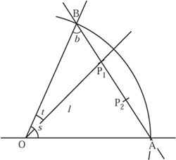
Figure 5.7. Attempting to divide an arbitrary angle into three: trisection.

The first thing to note is that (i) the angle b is equal to (π − s) and (ii) the length

BP₁ = sin (s.)

From this and the cosine rule we can establish that

l² =1 − Sin (s)²,

and in turn from the sine rule that

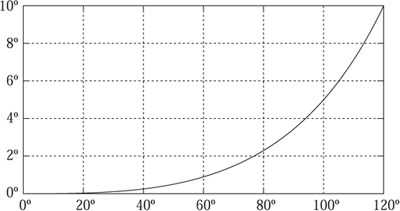
Figure 5.8. The error s − t against angle t when approximately trisecting an angle.

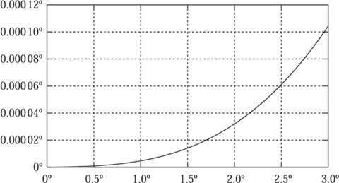
Figure 5.9. The error s − t against angle t when approximately trisecting a small angle.

This formula gives the exact relationship between s and t For values of s between 0° and 120°, the graph of the error, that is the difference between s and t, is shown in figure 5.8. Notice that for s between 0° and 60°, the actual error is less than 0.9°, but the central angle of the triplet has an error of about 1.8°. This is an accuracy which most people would be hard pushed to achieve using a normal protractor, so that for practical purposes with small angles this method will probably suffice; indeed figure 5.9 shows the error for values of s between 0° and 3°. A word of caution though. Trying to divide a short line exactly into three is also difficult. Here, proportional dividers can help. Indeed, pricking the surface with the points of such dividers can provide more accurate locations for the points than a pencil line would provide.

Figure 5.10. Details of angle trisection with a marked ruler.

This initial method does not work exactly, and although we do not prove it here, using only Euclidean constructions it is impossible to trisect an arbitrary angle exactly. Despite this unfortunate fact, there are even better approximate methods using only a ruler and compass. Some give extremely good approximations that are certainly better than any protractor. The method of Fahmi (1965) is a typical example.

5.6 Trisecting an Angle by Other Means

There are other ways to exactly trisect an arbitrary angle, and in this section we begin by showing how specialized the setting of ruler and compass really is. We do this by adding one extra tool. This is simply a straight edge marked with two points a distance r apart. We could take r to be 1, but in fact this does not matter—any two marks on the ruler will suffice. So, this modified straight edge is really the most basic of all rulers. Using this extra tool we explain how to trisect an arbitrary angle s.

We start by drawing a baseline and another line between which lies the angle s (see figure 5.10). On this we draw a circle, centred at the intersection of the lines and with a radius r. Place the marked ruler with the edge running through the point A and so that the distance BC is the marked distance r. We will examine the angle at t.

Figure 5.11. Trisecting an arbitrary angle s.

To determine t, we draw a further radius to where the line AC cuts the circle at B and mark the angles a, b and c as shown in figure 5.11. Since the two triangles AOB and OBC are isosceles, we have that

2t + c = b + c,

so b = 2t. Next

2b + a = s + a + t,

so 3t = s.

This is known as Pascal’s angle trisector, and we shall describe a simple mechanism that incorporates it in the next section.

5.7 Trisection of an Arbitrary Angle

Fortunately, from a practical point of view, you can forget about protractors and the impossibility of trisecting an angle by Euclidean constructions. In this section we shall show a way to do it and much more besides by means of a simple linkage. The linkage can be made without the need for measurement, its actual size being dictated solely by the available materials. It consists of two straight channels or guides of cross-section hinged together, some pivots that can slide in these guides freely without wobbling, and a set of links. The critical feature is that the centre of the linkage pin must lie on the centre line of the guides. The links should also all be the same length.

Figure 5.12. Dividing an angle by five.

Figure 5.13. Generalizing the trisection construction.

Only simple geometrical knowledge is needed to understand how it works. First recall that the base angles of an isosceles triangle are equal. Second we note that the extension angle of a triangle equals the sum of the two opposite internal angles. We shall adopt the convention that links are shown as broad lines and the centre lines of the guides as thin lines. The linkage pin acts as a pivot, marked P₀, and is used in all constructions.

Three sliding pivots are needed, together with three links. We can see from figure 5.13. In each case the final angle can be divided into equal parts.

Figure 5.12 shows that the angle

P₂P₀P₁ = C₁P₄P₅.

In the model in figure 5.13, the angle between the guides is not fixed, indeed it would be useless if it could divide only one particular angle between the guides. The numbers of pivots and links used is determined not by geometry but by their physical sizes. Unless they are small the maximum potential number of links is about nine or eleven.

Figure 5.14. Constructing 60°.

Figure 5.15. Constructing 36°.

A whole range of other geometrical games can be played if the linkages are put together in such a way that it becomes a rigid framework. In a rigid framework the angles are fixed. The game is to find a framework containing a specific angle, such as the construction of 60° shown in figure 5.14. The equilateral triangle made by the three links cannot be deformed and so the angle is set at 60°. All this is obvious, so we now add two more pivots to these links as shown in figure 5.15. As with the angle dividers we apply the properties of isosceles triangles to find

C₁P₀C₂ = 36°

Noticing that 60° 180° and that 36° = 180° points the way to generalizing this construction. Indeed, we do find that if we continue the pattern in a natural way,

Figure 5.16. Constructing 90° with external supports.

where 2k + 1 equals the number of links and 2k is the number of pivots. In principle, then, we have a means of constructing all the odd unit factors of 180°, although the same limitation is imposed by the physical size of the links and pivot slides.

Setting the guides to an even unit fraction of 180° is a completely different story, and there is no general method. The best we can do is 30°, or 180°. If we make two sets of linkages, we can subtract angles, but this is not all that helpful. Instead we go back to one linkage, but this time we will make use of some more pivots that can lie outside the guides, and construct rigid frameworks for 90° and 45°. For example, one way to construct 90° is to use two external supports and seven linkages: see figure 5.16.

Accepting that these are valid constructions, we can look back at 45° and see that we have constructed an angle tan^-1(1), so we could also form tan^-1() or, more generally, tan^-1(1 /n), where n is the number of links lying along the bottom guide. There are many other possibilities here—you can amuse yourself by finding them.

Figure 5.17. The origami trisection of EBC.

Figure 5.18. Proving that the construction trisects the angle.

5.8 Origami

Another way to trisect an arbitrary angle is using origami, something you could try out for yourself with an ordinary square of paper.

To trisect an angle take a square ABCD and on the edge AD mark a point E as shown in figure 5.17. Our task is to exactly divide the angle EBC into three. To construct this angle we proceed as follows. First choose a point F on the line AB and fold the line FG parallel to BC. Next, mark the point H where B meets the line and unfold the square. Now create a diagonal fold so that the point H lies on the line BE and the point B lies on the line FG. Where these points meet the lines mark H′ and B′, respectively. Again, unfold the square. Our claim, which we shall prove in a moment, is that the angle EBC is exactly three times the angle B′BC.

We first note that the distance BH is identical to B′H′. Furthermore, this distance is twice the distance FB = B′I. Next, note that the angle FBB′ = BB′I, and furthermore this angle is also equal to BB′H′. If we drop a perpendicular to B′H′ through B, we see that the three right-angled triangles shown in figure 5.18 are congruent. Hence the angle EBC is exactly three times the angle B′BC.