Chapter 6

FALLING APART

Humpty Dumpty sat on a wall.

Humpty Dumpty had a great fall.

All the King’s horses and all the King’s men

Couldn’t put Humpty together again.

Nursery rhyme

 

 

In this chapter we discuss mathematical jigsaws based on plane dissections and other solid models. Not only are these fun, but they also illustrate some important basic mathematical results. Mathematical dissections such as these all rely on the concepts of area and volume. We are concerned here with simple geometric shapes but we shall address the more general problem of measuring the area of an irregular shape in chapter 8.

6.1 Adding Up Sequences of Integers

There is a story about the famous mathematician Carl Friedrich Gauss (1777–1855) that while at primary school he was able to add the numbers from 1 to 100 in his head, and simply wrote the answer on his slate. He did this by noticing the following pattern, which can be adapted to add together the first n integers. That is to say,

1 + 2 + 3 + 4 + . . . + n.

The idea is simply to write the numbers twice, one list on top of the other but with the order reversed:

Notice that the total in each column is n + 1, and there are n such columns. Thus

This result may easily be seen by taking two sets of rectangular rods, consisting of one of each length from 1 to n, and pairing them up, so that the longest, i.e. that of length n, is paired with the shortest, i.e. that of length 1. (Sets of coloured rods, known as Cuisenaire rods, are standard equipment in many primary classrooms and can be easily employed for this purpose.) This is illustrated in plate 13. For somewhat obvious reasons the numbers n(n +) are sometimes referred to as triangular numbers.

Next we turn our attention to summing the cubes. That is to say adding

1³ + 2³ + 3³ + . . . + n³.

It is possible to prove that

1³ + 2³ + 3³ + . . . + n³ = (1 + 2 + 3 + . . . + n) ²,

which is sometimes expressed by saying that ‘the sum of the cubes of 1 to n is the same as the square of their sum’. This is known as Nicomachus’s theorem, and is attributed to Nicomachus of Gerasa, who is believed to have proved it around 100 C.E. In fact, our first result can be used here to show that this equals n²(n + 1)². Figure 6.1 shows one particularly satisfying illustration of why this is true, in the case n = 4. Although some of the squares do overlap, the total area is (1 + 2 + 3 + 4)². If we count the individual squares we see that

1 ×1² + 2 ×2² + 3 ×3² + 4 ×4² = 1³ + 2³ + 3³ + 4³ = (1 +2 +3 +4)².

We have missed out summing the squares of the integers. It is also possible to prove that

Since this is a cubic in n, and contains the fraction , one naturally considers whether it is possible to arrange six sets of flat squares into a box shape. Each set consists of one unit square, one 2×2 square, one 3×3 square, etc. And, indeed, if one has the patience to cut out the required number of unit cubes and stick them into squares, this can be done. For example, taking n = 5 we can find an arrangement of these squares into a 5×6×11 block. Actually, an even more surprising and satisfying three-dimensional jigsaw can be made with six copies of an off-centre pyramid, in which the number of steps can be made arbitrarily large. This is illustrated in plate 14.

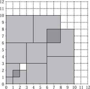
Figure 6.1. Summing the cubes of the first four integers.

Anyone who makes six copies of this pyramid and puts them together will see that another hybrid three-dimensional jigsaw can be made from only three of these and a stepped triangular piece taken from half of the illustration that 1 + 2 + . . . + n = n(n + 1), shown in plate 13.

6.2 Duijvestijn’s Dissection

Ideally we would like to make a flat square jigsaw consisting of smaller squares. If we want to take a complete sequence we need to know whether it is possible to cut a square up into a sequence of other squares of size 1² ,..., n². This will only be possible if the total area is a square number. That is to say, if

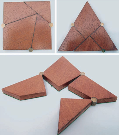
Plate 1. Dudeney’s dissection

Plate 2. Chebyshev’s straight-line mechanism, in original and alternative forms.

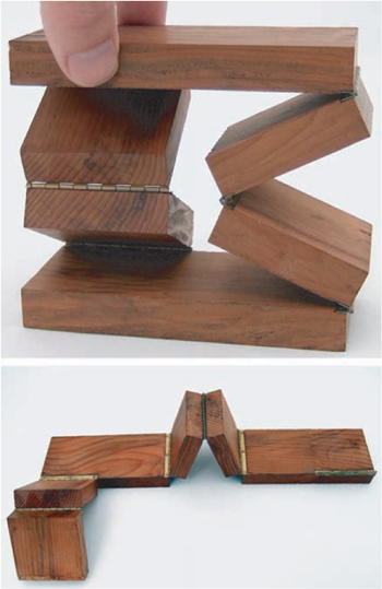
Plate 3. Sarrus’s linkage.

Plate 4. Two forms of Peaucellier’s linkage.

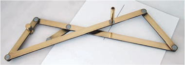
Plate 5. Hart’s straight-line linkage.

Plate 6. Hart’s A-frame linkage.

Plate 7. Scott Russell’s linkage.

Plate 8. The Grasshopper linkage.

Plate 9. Rolling two parabolic templates to draw a straight line.

Plate 10. General four-bar linkages.

Plate 11. Chebyshev’s six-bar paradoxical mechanism.

Plate 12. A model which includes Pascal’s angle trisector.

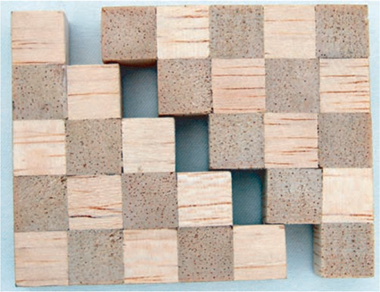
Plate 13. Illustrating the sum from 1 to n.

Plate 14. Summing the squares of the numbers from 1 to n.

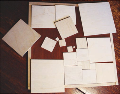
Plate 15. Duijvestijn’s dissection.

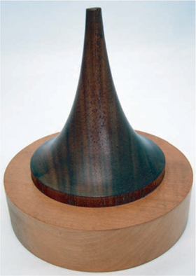
Plate 16. A hemipseudosphere.

Plate 17. Three-dimensional shapes of constant width in wood, brass and plastics.

Plate 18. Three-dimensional shapes of constant width.

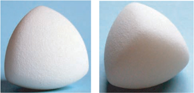
Plate 19. A three-dimensional shape of constant width based on a regular tetrahedron.

Plate 20. Watts’s drill that cuts a square hole.

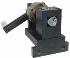
Plate 21. A drill that cuts a square hole.

Plate 22. A Reuleaux rotor.

Plate 23. The Magnameta Oil Tonnage Calculator.

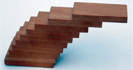
Plate 24. A balancing stack of wooden blocks, 90% to the point of collapse.

Plate 25. Balancing stacks of wooden blocks, 50%, 70% and 90% to the point of collapse.

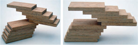
Plate 26. Twisting part of the stack.

Plate 27. Self-righting (left) and over-balanced (right) stacks.

Plate 28. A ‘two-tip’ polyhedron.

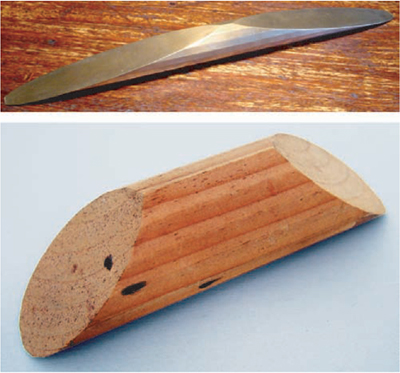
Plate 29. Uni-stable polyhedra.

Plate 30. Slotted discs.

Plate 31. Alternatives to two slotted discs.

Plate 32. Slotted ellipses.

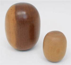
Plate 33. Two super-eggs.

1² + . . . + n² = n(n + 1 (2n + 1) = r²

for some integer r. In fact there are only two integers n for which this is possible: n = 1 and n = 24 (giving r = 70). That is to say, 1² + 2² + . . . + 24² = 70². However, simply because the shapes have the same area does not mean we can cut a 70 × 70 square up into twenty-four squares, one of each size. To illustrate the sort of things that go wrong, try to explain why it is impossible to arrange thirty-one 2 × 1 dominoes on a chess board which has had two diagonally opposite corner squares removed. Such a dissection of the square would make a stunning, if rather difficult, jigsaw puzzle!

However, there are many dissections of a large square into squares that do not use a regular sequence of smaller squares. These kinds of dissections make excellent jigsaws, particular those which are squares made up of other squares, no two of which are the same. The smallest such dissection was first discovered by A. J. W. Duijvestijn and published in Scientific American in 1978. This consists of twenty-one squares with sides of length 2, 4, 6, 7, 8, 9, 11, 15, 16, 17, 18, 19, 24, 25, 27, 29, 33, 35, 37, 42 and 50. These fit into a square with sides of length 112. It is known that this is the unique dissection with twenty-one different squares and that there is no such dissection of a square into fewer squares. A jigsaw using Duijvestijn’s dissection is shown in figure 6.2.

The smallest square in the dissection has sides with length one unit, and the smallest size convenient for a piece is 5 mm ×5 mm, although even this can be difficult to handle. With this scale the largest piece is 405 mm × 405 mm, with the complete puzzle measuring 825 mm × 825 mm. To appreciate how accurately the puzzle needs to be made, notice that if we draw a horizontal line through the centre of the square it crosses six pieces, whereas a vertical line through the fifty-five unit square cuts only three pieces. Evidently each piece must be made very accurately if the whole puzzle is to fit together in a satisfying way, without unseemly gaps—and do not forget that they must fit equally well in any of the four rotational positions and on both sides. Straight edges and right angles can be checked very accurately with an engineer’s or carpenter’s square, and their size with Vernier callipers.

The most attractive feature of Duijvestijn’s dissection as a plan for a real puzzle is not so much that it requires the minimum number of pieces but that the ratio of the side lengths of the largest to the smallest is 25:1—smaller than other published dissections. This is of great practical significance, and taking the lengths of the sides of the smaller square to be 5 mm, the largest is 125 mm and the whole square is only 280 mm, an altogether more convenient size. Three millimetre plywood is probably the easiest material to use. A completely different technique from that used in section 1.2 was needed for making this dissection. Start by cutting squares slightly oversize and bring one side straight by carefully sanding, then, with the aid of an engineer’s square, do the same to the second side. We need to do some accurate measuring for the next two sides and rather than use a ruler use Vernier callipers open to the exact size required. Still checking for squareness and straightness, test with the callipers: the size will be right when the jaws of the callipers just, and only just, drop across the square. Check the fourth side for squareness from both ends, and sand down to the point where the callipers drop: you will have one accurate square. It is best to start with the largest square so that if you end up under size it can be used for another piece. The final sizing is best carried out with wet and dry paper glued to a flat strip of wood. We have found that making three or four squares in one session is enough, as it does require extreme concentration. The result, however, is well worth the effort.

Notice that to complete both these patterns one takes the greedy approach. In terms of Willcocks’s dissection, this means that we begin with the largest two squares in opposite corners. Then we pack the next four largest to completely fill opposite edges. Next, the position of the 39-unit square should be clear, leaving a relatively small number left to fit in. However, the greedy approach is not always best. For example, assume we have five suitcases, four are 1 × 1 and one is slightly larger at 1.01 × 1.01. If we want to pack as many suitcases as possible into a 2 × 2 car boot, the greedy approach is clearly the worst, since only one will fit! When and when not to take the greedy approach is often far from obvious. Scheduling, ordering and packing problems are often mathematically very similar, and they are of huge practical importance.

Figure 6.2. Willcocks’s dissection.

6.3 Packing

In general, packing problems in mathematics are very difficult. By this, we do not mean difficult conceptually, but difficult in a computational way. Imagine you are going to use an exhaustive search method and look at every possible combination. There are just so many ways one could try to pack that the computation may effectively never finish. For example, imagine you want to arrange n different items in a queue. There are n ways of choosing the first. For each of these there are (n − 1) ways for the second. Repeating this we see that in total the number of arrangements is

n × (n − 1) × (n − 2) × . . . × 3 × 2 × 1 = n!.

The function n! (pronounced ‘n-factorial’) grows very rapidly indeed: for example, 65! ≈ 8.2 ×10⁹⁰, which is quite significantly more ways than there are particles in the known universe. Much more modestly, if you wanted to display all possible arrangements of only a dozen items, at the rate of one arrangement per second, it would take you 12! = 479 001 600 seconds to do so, which is over 15 years.

One modern and exciting solution to this problem is to use strands of RNA (ribonucleic acid). These are complex molecules that react together to form long chains. The order in which this chain forms is random, and a test tube will contain some 10¹⁹ such molecules. This random linking is effectively like a parallel computation, with each combination being formed simultaneously. In many of these problems, recognizing a solution when you have it is comparatively simple. We can see when the parts ‘fit’ together. The problem is finding out whether or not a sequence corresponding to a mathematical solution is present at the end. Hence, if you look at which strands of RNA are produced in the reaction, you can find out whether a solution to your problem is there. This is done by a chemical reaction, very much like DNA fingerprinting. One of the pioneering papers in this new and exciting computational field is Adleman (1994).

6.4 Plane Dissections

In general, given any two polygonal figures of equal area, there exists a dissection between them using only a finite number of pieces. This result is proved in a number of stages, and we sketch an informal argument. The important observations are that (i) any polygonal figure may be divided into triangles and (ii) any triangle may be dissected and rearranged into a rectangle of prescribed base length. We can use a stack of such rectangles as intermediates between the two polygonal figures. Of course, such an argument has much detail to fill in, and in general this procedure will result in a large number of pieces. Perhaps a more interesting problem would be to find the minimum number of pieces needed for a dissection between two polygonal shapes. This problem appears to be very difficult and is currently unsolved in the general case. An extensive treatment of the history and mathematics of dissections is given in Frederickson (1997), with special hinged dissections covered in Frederickson (2002).

Figure 6.3. The Pythagorean theorem.

We cannot resist including another illustration of the Pythagorean theorem. In figure 6.3 is satisfying because it is immediately obvious that the area of the unshaded region on the left is c², and the areas of those on the right are a² and b². The link between them is achieved by moving four copies of the original triangle itself. The figure on the left shows that (a + b)² = c² + 2ab. On the left we have (a + b)² = 2 ab + a²+ b ². A wooden model of this is illustrated in figure 6.4.

It should be noted that modelling a geometric dissection always requires precise work, although the model shown in figure 6.4 was made without any measurement of length. The four triangles were cut from 1.5 mm plywood and finished clamped together to make sure they were all the same and were truly right-angled triangles with straight edges. The tray was made to fit, again without measurement.

Figure 6.4. A model illustrating the Pythagorean theorem.

6.5 Ripping Paper

We would like to propose another experiment in this section. You will need a couple of sheets of paper for this and you will be tearing these up into pieces.

For the first experiment take a square of paper and rip it in half. Take the remainder and tear this in half again. Continue this process forever, or at least until your remaining piece becomes too small, at which point you will be forced to let a thought experiment take over. Now, what you have strongly suggests that

This is an impression that figure 6.5 should reinforce.

Next take the other piece of paper and tear this into three equal bits and start to make two piles with two of the pieces. Take the third and rip this into three more equal size pieces and add one to each of the piles. Each pile now has

Again, tear up the remaining bit into three and add one new bit to each pile. Keep doing this, and at each stage tear the paper you are holding into three pieces of equal size. Once the experiment is complete you will have two identical piles, each of which suggest that

Figure 6.5. Infinite division of the square into successive halves.

You might like to sketch a counterpart of figure 6.5 that corresponds to this new experiment.

In each of these experiments we end up creating a pile of paper and then adding up the total area each piece represents. In the resulting sums, each term is a certain number of times the preceding term. In the first experiment we had a half and in the second a third. We could use any number as the multiplying factor and, for example, consider a sum such as

1 + 2 + 4 + 8 + 16 + . . . .

All of these are known as geometric sums. Such sums have direct applications in many areas of mathematics, including the calculation of the total compound interest in a regular savings account.

Figure 6.6. Illustrating the convergence of a general geometric progression, r = .

In a general case the multiplier is r. For fixed r ≠ 1 and n it is a standard result that

When r = 1 the value of (6.5) is simply n.

This series is very important indeed and will give us our first bite at infinity. When − 1 < r and r < 1 we can prove that r ⁿtends to zero as n tends to infinity. That is to say, as n gets larger and larger, the values of r ⁿ eventually remain arbitrarily close to zero. This allows us to make sense of the limit

The above is an infinite sum, to which we have ascribed a definite value, as was suggested by the experiment. Taking r = and subtracting the first term gives us the famous result (6.3).

The illustration of the case r = in figure 6.5 is essentially a special trick and does not generalize. However, the diagram shown in figure 6.6, given by Casselman (2000), allows us to see this for any 0 < r < 1. The squares of side 1, r, r ², etc., are simply placed side by side. Where the line that connects all the top left corners intersects the baseline is the sum of the progression. The case for r = is shown in figure 6.6.

Actually, forgetting the restriction - 1 < r < 1 in the identity is an excellent source of mathematical nonsense. For example, taking r = 2 gives

and taking r = −3 gives

The modern student of analysis would immediately object that the partial sums do not converge; however, Euler (2000, section 109) does not dismiss their importance entirely.

However, it is possible, with considerable justice, to object that these sums, even though they seem not to be true, never lead to error. Indeed, if we allow them, then we can discover many excellent results that we would not have if we rejected them out of hand. Furthermore, if these sums were really false, they would not consistently lead to true results; rather, since they differ from the true sum not just by a small difference, but by infinity, they should mislead us by an infinite amount. Since this does not happen, we are left with a most difficult knot to unravel.

6.6 A Homely Dissection

The final light-hearted dissection that we discuss can hardly be described as a mathematical model, or even a model, at all, but it does show that when no material is lost with a shearing cut by knife or scissors a more relaxed approach is possible. It can be demonstrated most easily on the breakfast table: it might even be construed as a lesson in table manners and be used in a book on etiquette. All that is required is a thin slice of bread cut from a square loaf and cut again diagonally to form a 90° isosceles triangle (see figure 6.7). Good manners dictate that it should be cut in half before attempting to eat it.

The most obvious cut is shown where D bisects AC. If AB and BC, the sides of the original loaf, are taken to have lengths of 1 unit, then the total area is , the length of the cut is ≈ 0.707, and the area of each piece.

Figure 6.7. An obvious way to cut toast.

Figure 6.8. Other ways of cutting a slice of toast.

The problem is to discover if there is a shorter cut that would still divide the slice into two equal areas, thus saving wear and tear on the plate and knife. However the cut is made, one of the 45° corners or the 90° corner will be in the triangular section and a quadrilateral will remain. Since the more promising solution looks to be to slice off the corner C (on the left-hand drawing) rather than B (on the right), we shall examine that possibility first (see figure 6.8). The area of the small triangle is

Hence ab = . Applying the cosine rule,

gives

Using calculus to find the maximum or minimum value we consider

Figure 6.9. A dissection of a cube into three identical yángm.

Therefore, ⁴ = and so ² = b . Hence, the triangle in which c is shortest is isosceles. The length of cut is therefore approximately 0. 6436, a saving of approximately 9% compared with the original 0. 7071. While we have not proved that this is a minimum we leave it to you to consider the case when we cut off the 90° angle at B. A 9% saving is a poor return for the effort of cleaning butter from a ruler, and such an approach to cutting the bread is so unorthodox that it might itself be considered to be a breach of etiquette.

6.7 Something More Solid

Of course we can cut up solids into pieces, as well as flat objects into jigsaws. Dissections of solids are generally much harder in practice. One exception is the dissection of a cube into three identical square-base pyramids, known as yángm, shown in figure 6.9. The three yángm can also be hinged together. The net shown in figure 6.10 can be constructed very simply using the following origami construction, which is given in Brunton (1973). It is indeed fortunate that we have this origami-type construction, since does not appear on many rulers, and measuring this length is necessary for the construction.

We start with a square ABCD, which surrounds the net. The procedure is as follows.

1. Fold along AC.
2. Fold DC on AC to find the point E on AD. (You should show that this point is in the correct place!)
3. Make a fold FG so that AB is perpendicular to AD through E.
4. Fold EH, parallel to DC. Where EH intersects AC mark on J.
5. Fold the two lines E H and F G, both parallel to AD, as shown in the bottom right of figure 6.11.

Figure 6.10. The net of a yángm.

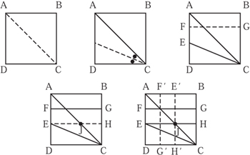
Figure 6.11. The construction steps for a yángm.

Since three identical yángm make a cube, their volume is one-third that of the cube. This result is actually considerably more general: the volume of any straight-sided pyramid is one-third of the base area multiplied by the vertical height. In chapter 8 we consider area in detail, and illustrate why the area of a circle is πr². Hence the volume of a circular cone must be