A fundamental problem in formal verification is determining whether two Boolean functions are functionally equivalent. A case in point is to determine whether a circuit, after timing optimization, retains the same functionality. Logical equivalence can be done on either combinational functions or sequential functions. Determining even combinational equivalence can be hard, such as deciding whether ![]() is equivalent to
is equivalent to ![]() . The second expression can be obtained from the first expression by shifting the complementation operation to the other literal of each cube. Although somewhat counterintuitive, these two expressions are functionally equivalent. Sequential equivalence is concerned with determining whether two sequential machines are functionally equivalent. One way to do this is based on combinational equivalence. First we minimize the two machines to eliminate redundant states, then we map their states based on one-to-one correspondence, and finally we decide whether their next-state functions are combinationally equivalent. The problem of combinational equivalence is a focus of this chapter.
. The second expression can be obtained from the first expression by shifting the complementation operation to the other literal of each cube. Although somewhat counterintuitive, these two expressions are functionally equivalent. Sequential equivalence is concerned with determining whether two sequential machines are functionally equivalent. One way to do this is based on combinational equivalence. First we minimize the two machines to eliminate redundant states, then we map their states based on one-to-one correspondence, and finally we decide whether their next-state functions are combinationally equivalent. The problem of combinational equivalence is a focus of this chapter.
A brute-force method to determine combinational equivalence is to expand the combinational functions in minterm form and compare them term by term. The minterm representation has the property that two equivalent Boolean functions have identical minterm expressions. This property in general is called canonicity of representation. A representation having the property is a canonical representation. In addition to minterm representation, maxterm and truth table are also canonical representations. One way to decide whether two functions are equivalent is to represent them in a canonical form. If their forms are identical, they are equivalent; otherwise, they are not equivalent. However, this method runs into the problem of exponential size, because the number of minterms or maxterms of a function can be exponential with respect to the number of variables.
The sum-of-products representation is more compact than minterm representation, but it does not reveal readily functional equivalence or unequivalence. As demonstrated by our previous example, the two functions have a completely different appearance, even though they are functionally equivalent. Thus, a second desirable property of a representation, besides canonicity, is compactness. Sum-of-products is more compact than truth table representation.
An ideal representation should be both canonical and compact. Because logical equivalence is an NP-complete problem, it is likely that all canonical representations are exponential in size in the worst case. However, a canonical representation is still useful if its size for many practical functions is reasonable. In this chapter we will look at BDDs as a representation of Boolean functions. Then we will examine how BDDs are used in determining functional equivalence. As an alternative to BDDs in checking equivalence, we will study SAT. Finally, we will examine symbolic simulation, to which BDDs and SAT are applicable.
A BDD is a directed acyclic graph (DAG) that represents a Boolean function. A node in a BDD is associated with a Boolean variable and has two outgoing edges. One edge represents the TRUE (1) value of the variable, and the other, the FALSE (0) value. The two edges point to other BDD nodes. Let’s call the node pointed by the 0-edge the 0-node and the node by the 1-edge, the 1-node. Using this convention, the left edge represents the 1 value of the variable and the right edge represents the 0 value. The node without an incoming edge (in other words, not being pointed to) is called the root of the BDD. A leaf node or terminal node, denoted by a square, is not associated with a variable and is a constant node that evaluates to either 0 or 1. The size of the BDD, denoted as |BDD|, is the number of nodes in the BDD. To evaluate a function represented by a BDD on a given value of its inputs, we start from the root and follow the edges to trace the path determined by the variable values. When a node is encountered, whether the right or left edge is followed is determined by the value of the variable of the node. For instance, at node x, the right edge is followed if x takes on value 0; otherwise, the left edge is followed. If the path arrives at terminal node 0, the function evaluates to 0. If the path arrives at terminal node 1, the function evaluates to 1.
Example 8.1
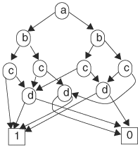
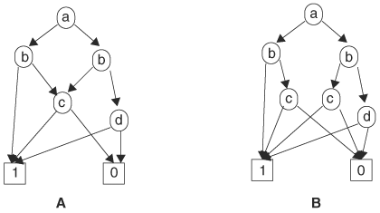
An example of a BDD is shown in Figure 8.1. By looking at Figure 8.1, we can determine that node a is the root of the BDD because it has no incoming edges. More than one node can represent the same variable. For example, there are two nodes representing variable b. The two square nodes at the bottom are terminal nodes, representing 0 and 1. For input value a = 1, b = 0, c = 1, we evaluate the function. Start at the root, which represents variable a. Because a = 1, we take the left edge and arrive at node b on the left-hand side. Because b = 0, we take the right edge and arrive at node c. Because c = 1, we follow the left edge and arrive at terminal node 1. Therefore, for a = 1, b = 0, c = 1, the function evaluates to 1. The path traced is P1. Note that variable d is not involved in this evaluation and this means the value of the function for this particular input combination is independent of variable d.
In this example we traced a path in a BDD from an input value. Conversely, we can select a path in a BDD and deduce from it the value of the function and the input value giving rise to the function value. For instance, consider path P2, which arrives at terminal node 0. Along the path, a takes on 0 because the right edge is taken, b takes on 1, and c takes on 0. This path implies that the function evaluates to 0 when a = 0, b = 1, and c = 1. In other words, cube ābc is in the off set of the function. Therefore, any path ending at terminal 0 represents a cube in the off set. Similarly, any path ending at terminal 1 represents a cube in the on set. Thus, we can derive the function this BDD represents. In sum-of-products form, we look at all paths ending at terminal 1. There are four paths. These four paths represent cubes ![]() ,
, ![]() ,
, ![]() and ab. Because each of these cubes causes the function to be 1, the function is a sum of these cubes:
and ab. Because each of these cubes causes the function to be 1, the function is a sum of these cubes:
To derive the function in product-of-sums form, we need to work on the off set. There are three paths ending at terminal 0. These paths represent cubes ![]() ,
, ![]() , and
, and ![]() :
:
Using DeMorgan’s Law, we can obtain the function in product-of-sums form:

The BDD rooted at node x represents a Boolean function f, and the 0-node represents the cofactor of the function, fx, and the 1-node, fx. This is because the function of the 0-node is derived from the root via the setting of x to 0, which is just ![]() . The same goes for the relation between the 1-node and fx. Consequently, to obtain the Boolean function of a BDD, one can apply the Shannon cofactor theorem in reverse. Once the functions at the 0-node and 1-node of a node have been computed to be g and h, then the function at the node is
. The same goes for the relation between the 1-node and fx. Consequently, to obtain the Boolean function of a BDD, one can apply the Shannon cofactor theorem in reverse. Once the functions at the 0-node and 1-node of a node have been computed to be g and h, then the function at the node is ![]() . This can be done from either the bottom up, starting from the constant nodes, or from the top down recursively. A top-down recursive algorithm is as follows:
. This can be done from either the bottom up, starting from the constant nodes, or from the top down recursively. A top-down recursive algorithm is as follows:
Derive Boolean Function from a BDD: BDDFunction(BDD)
Input: a BDD
Output: the Boolean function represented by the BDD
x = root of BDD.
If x is a constant, return the constant.
Let y and z be the 1-node and 0-node respectively of x.
Return xBDDFunction
 BDDFunction(z).
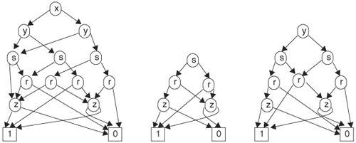
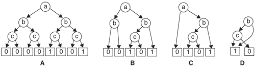
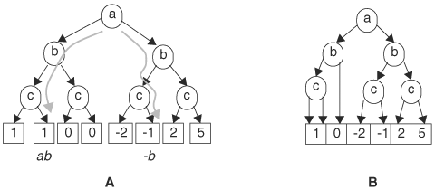
You may observe that the paths in a BDD determine the cubes in the function’s on set and off set, and a path (consisting of a sequence of nodes) produces a cube regardless of the order in which the nodes appear along the path. For instance, path a,right; b,right; and c,right gives the same cube as path b,right; c,right; a,right in another BDD. The two BDDs shown in Figure 8.2 represent the same function even though the two graphs do not resemble each other. Using the previous path tracing technique, we can verify that the two BDDs represent the same function. Consider the BDD in Figure 8.2B. There are six paths that end at terminal node 1. These paths produce cubes dc, ![]() ,
, ![]() ,
, ![]() ,
, ![]() and
and ![]() . Therefore, the function is
. Therefore, the function is

which is identical to the function given by the BDD in Figure 8.2A. You may note that between the two BDDs, the order of the variables along the paths is different. In the first BDD, along any path, the order of variables is a, b, c, d, whereas in the second BDD, the order is d, c, b, a. One of our objectives is to find a canonical representation. In this case, two functionally equivalent functions should have graphically identical BDDs. Therefore, to achieve canonicity, an ordering of nodes must be imposed. An ordered BDD (OBDD) is a BDD with variables that conform to an ordering. Given a variable ordering <, an OBDD with the ordering is a BDD with the restriction that for any path in the OBDD containing variables x and y, node x is an ancestor of node y if x < y.
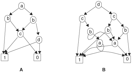
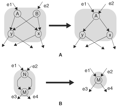
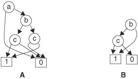
With an ordering imposed on variables, we have to consolidate many different BDDs of the same function. However, the remaining OBDDs are not yet unique. For instance, the two OBDDs in Figure 8.3 have the same variable ordering and represent the same function, but they are not graphically identical. Note that the two c nodes in Figure 8.3B can be merged because these two nodes represent the same function—namely, c. Once these two c nodes are merged, the two OBDDs are now identical. Indeed, it can be proved that if the following irredundancy conditions are satisfied on an OBDD, then the OBDD is canonical:
There are no nodes A and B such that they share the same 0-node and 1-node.
There is no node with two edges that point to the same node.
If the two nodes in condition 1 do exist, the function represented at nodes A and B is equivalent, according to the Shannon theorem, and thus the nodes should be combined. That is, if condition 1 is violated, then nodes A and B can be merged into a single node. If a node with two edges points to the same node, it means that the value of the variable at the node, whether 1 or 0, has no effect on the outcome, because the same node is encountered for either value of the variable; hence, this node can be ignored. That is, if condition 2 is violated, the node can be eliminated. The two transformations, merge and eliminate, are illustrated in Figure 8.4. With the merge transformation, when a node is merged with another, all incoming edges are redirected to the new node, and the node is deleted. In Figure 8.4A, node A and node B are to be merged; node A is picked as the new node and node B is deleted. The incoming edge of node B is redirected to node A. In eliminate transformation in Figure 8.4B, both edges of node N point to the same node M, and hence node N is redundant. Node N is removed and its incoming edges are redirected to node M as shown.

An OBDD satisfying the two irredundancy conditions is called a reduced OBDD (ROBDD). The major property of ROBDDs is canonicity, as stated in Theorem 8.1.
Once Boolean functions are represented using BDDs, Boolean operations are translated into BDD manipulations. In this section we will study algorithms for constructing BDDs from a Boolean function and a circuit, and for computing various Boolean operations using BDDs.
Construction algorithms build a BDD for a function or circuit. The first question is whether any Boolean function has a BDD representation. The answer is affirmative because a BDD can be constructed for any function based on the Shannon cofactor theorem. According to the cofactor theorem, any function can be expressed as ![]() . Therefore, we can create a BDD with node x with a 1-edge that points to fx and a 0-edge that points to
. Therefore, we can create a BDD with node x with a 1-edge that points to fx and a 0-edge that points to ![]() , and then recur the procedure on fx and
, and then recur the procedure on fx and ![]() until the function is a constant, as demonstrated in Example 8.3.
until the function is a constant, as demonstrated in Example 8.3.
Example 8.3
Construct a BDD for ![]() . Let’s choose variable ordering a < b < c. First we compute cofactors of f with respect to variable a. fa and fā are equal to
. Let’s choose variable ordering a < b < c. First we compute cofactors of f with respect to variable a. fa and fā are equal to ![]() and (bc) respectively. Thus,
and (bc) respectively. Thus, ![]() . Create node a and point its edges to fa and fā. Repeat the same procedure for the two cofactors:
. Create node a and point its edges to fa and fā. Repeat the same procedure for the two cofactors: ![]() is cofactored as
is cofactored as ![]() ; thus, fab = 1 and
; thus, fab = 1 and ![]() . Create node b and point its two edges to
. Create node b and point its two edges to ![]() and fab. The other cofactor, bc, is cofactored as b(c); thus,
and fab. The other cofactor, bc, is cofactored as b(c); thus, ![]() and
and ![]() . Create another node b and point its edges to
. Create another node b and point its edges to ![]() and fāb. Function c is
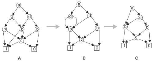
and fāb. Function c is ![]() . Create another node b and point its edges to 0 and 1. The BDDs for these cofactors are shown in Figure 8.7A. Connecting all these BDDs together, we have a BDD in Figure 8.7B. The cofactors are labeled in the BDD to illustrate the relationship between cofactor functions and BDD nodes. Then we apply the merge and eliminate transformations on the BDD to derive an ROBDD, as shown in Figure 8.7C.
. Create another node b and point its edges to 0 and 1. The BDDs for these cofactors are shown in Figure 8.7A. Connecting all these BDDs together, we have a BDD in Figure 8.7B. The cofactors are labeled in the BDD to illustrate the relationship between cofactor functions and BDD nodes. Then we apply the merge and eliminate transformations on the BDD to derive an ROBDD, as shown in Figure 8.7C.

Figure 8.7. Constructing BDDs using Shannon cofactoring. (A) BDD nodes and Shannon cofactors. (B) Connect BDD nodes. (C) Reduce BDD.
The major drawback of this method is the exponential number of operations. For the first variable, two cofactor functions are created. For the next variable, four cofactor functions are created, and so on. In general, 2n cofactor functions are created for n variables. In practice, BDDs are built from the bottom up, starting from variables or primary inputs of a circuit. As the building process progresses, a dynamic programming technique keeps track of the intermediate functions being built and returns the result if an intermediate function has already been built. This reuse strategy cuts down runtime substantially.
Let’s look at the bottom-up construction process. Then we will see how dynamic programming helps to reduce runtime. From the start, BDDs are built for the variables, then for simple expressions made of the variables, followed by more complex expressions made of the simple expressions, until the function is completed.

The complexity of BDD construction in general depends on variable ordering. However, there are functions with BDD sizes that are exponential for any variable ordering. In practice, however, many functions have polynomial sizes for some variable orderings. We will revisit the issue of variable ordering in a later section.
Reduction operation transforms a BDD into a reduced BDD by applying recursively the merge and eliminate transformations on the BDD until the irredundancy conditions (see page 393) are met. The complexity of making a BDD canonical is O(|BDD|), because each node is examined a fixed number of times in the transformations. To reduce a BDD with variable order π, we apply the merge and eliminate transformations to BDD nodes following the reverse ordering of π. Initially, we apply the emerge transformation to all constant nodes. Then we apply the merge and eliminate transformations to all BDD nodes of the last variable in π. Next, we repeat the transformations on the next-to-the-last variable and so on, until all variables are examined. At the end, the resulting BDD satisfies the irredundancy conditions. For instance, the BDD in Figure 8.7B does not satisfy the irredundancy conditions. We start out by combining the constant terminal nodes, which then reveal that the two c nodes have their respective 1-nodes and 0-nodes pointing to the same nodes. We then apply the transformations to the c nodes and combine them. Finally, we repeat these actions on the b nodes. At the end, the resulting BDD shown in Figure 8.7C satisfies the irredundancy conditions and hence is canonical.
Restriction operation on a function sets certain variables to specific values. For example, restricting x to 0 and y to 1 in ![]() produces
produces ![]() . This operation can be easily done on BDDs. To restrict variable v to 1, simply redirect all incoming edges to BDD nodes labeled v to their 1-nodes. Similarly, restricting v to 0 redirects all incoming edges to the 0-nodes. After the edges are redirected, it is possible that redundant nodes and equivalent nodes may appear. Thus, the reduction operation is called to reduce the BDD. The BDD nodes labeled v still exist in the BDD, but they have no incoming edges. To clean up, successively remove all nodes, except the root, that have no incoming edges.
. This operation can be easily done on BDDs. To restrict variable v to 1, simply redirect all incoming edges to BDD nodes labeled v to their 1-nodes. Similarly, restricting v to 0 redirects all incoming edges to the 0-nodes. After the edges are redirected, it is possible that redundant nodes and equivalent nodes may appear. Thus, the reduction operation is called to reduce the BDD. The BDD nodes labeled v still exist in the BDD, but they have no incoming edges. To clean up, successively remove all nodes, except the root, that have no incoming edges.

When functions are represented by BDDs, operations on the functions translate into operations on BDDs. For example, f AND g becomes BDD(f) AND BDD(g). Here we examine various operations on BDDs. First we encounter the ITE (if–then–else) operator on Boolean functions A, B, and C: ITE(A, B, C) = AB + ĀC. Note that the function represented by a BDD node, say x, is a special case of an ITE operation; the function of the node can be written as ITE(x, function at 1-node, function at 0-node). The ITE operator notation also has the added convenience of relating to BDD nodes. For example, ITE(x, y, z), where x, y, and z are BDD nodes, simply represents BDD node x with its 1-edge pointing to node y and its 0-edge pointing to node z. The ITE operator encompasses all unary and binary operators. Table 8.1 lists some common Boolean operators and their corresponding ITE representations.
Table 8.1. ITE Operator Representation of Boolean Operators
Operator | ITE form |
|---|---|
| ITE(X,0,1) |
XY | ITE(X,Y,0) |
X+Y | ITE(X,1,Y) |
X ⊕ Y |
|
MUX(X,Y,Z) | ITE(X,Y,Z) |
composition, f(x,g(x)) | ITE(g(x),f(x,1),f(x,0)) |
∃xf(x) | ITE(f(1),1,f(0)) |
∀xf(x) | ITE(f(1),f(0),0) |
The complementation operation, ![]() , simply switches the 0 and 1 constant nodes. Composition of Boolean functions substitutes a variable in a function with another function and can be computed as follows. Composing f(x,y) with y = g(x), giving f(x, g(x)), is equivalent to f(x,1) when g(x) = 1 and f(x,0) when g(x) = 0. Symbolically,
, simply switches the 0 and 1 constant nodes. Composition of Boolean functions substitutes a variable in a function with another function and can be computed as follows. Composing f(x,y) with y = g(x), giving f(x, g(x)), is equivalent to f(x,1) when g(x) = 1 and f(x,0) when g(x) = 0. Symbolically,
which is ITE(g(x),f(x,1),f(x,0)). The existential and universal quantification operators are

which consist of restriction, and OR and AND operations. The existential quantification ∃xf(x) = f(1) + f(0) has the interpretation that there exists a value of x such that f(x) holds. Because x is binary, either f(0) or f(1) must hold. In other words, ∃xf(x) = f(1) + f(0). Similarly, the universal quantification means that for all values of x, f(x) holds. That is, f(0) and f(1) must hold; hence, ∀xf(x) = f(1) · f(0).
Therefore, once we have an algorithm to perform ITE operations on BDDs, we can perform any unary and binary Boolean operations on BDDs. The key to ITE operations is based on the following identity:

which shows that the problem can be reduced to a smaller problem by cofactoring with respect to a variable, and it lends itself to a recursive algorithm. When calls to ITE(Ax, Bx, Cx) and ITE(![]() ,
, ![]() ,
, ![]() ) return, a BDD node x is created and its two edges are pointed to ITE(Ax, Bx, Cx) and ITE(
) return, a BDD node x is created and its two edges are pointed to ITE(Ax, Bx, Cx) and ITE(![]() ,
, ![]() ,
, ![]() ). The recursion stops when it reaches a terminal case for which the ITE operation is trivial. The terminal cases are the ITEs that are equal to either constants, one of its operands, or complement one of its operands. For example, these are terminal cases: ITE(1,X,Y), ITE(0,Y,X), ITE(X,1,0), ITE(Y,X,X), all of which are equal to X, and ITE(1, 1, Y), ITE(0, Y, 1), ITE(X, 1, 1), all of which are equal to 1.
). The recursion stops when it reaches a terminal case for which the ITE operation is trivial. The terminal cases are the ITEs that are equal to either constants, one of its operands, or complement one of its operands. For example, these are terminal cases: ITE(1,X,Y), ITE(0,Y,X), ITE(X,1,0), ITE(Y,X,X), all of which are equal to X, and ITE(1, 1, Y), ITE(0, Y, 1), ITE(X, 1, 1), all of which are equal to 1.
This recursive operation is shown in Figure 8.10. The triangles are input BDDs of functions A, B, and C. Figure 8.10A is operation ITE(root(A), root(B), root(C)), where we use notation root(A) to emphasize that the operand is the root node of BDD A. The first variable x selected for cofactoring is the earliest ordered root variable of A, B, and C. Figure 8.10B depicts the situation after one recursive call: A BDD node for variable x is created and two ITE calls are invoked on the 1-node and 0-node of the root of BDD A, B, and C; that is, the two recursive calls are as follows, the operands of the ITE operator being BDD nodes: ITE(root(Ax), root(Bx), root(Cx)) and ITE(root(![]() ), root(
), root(![]() ), root(
), root(![]() )).
)).
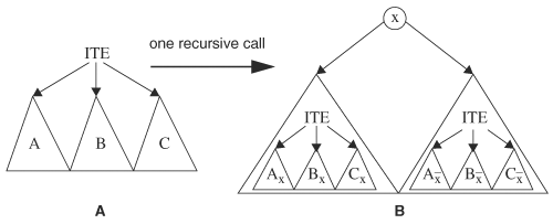
Figure 8.10. Recursive algorithm for computing the ITE operator. (A) Before an ITE call (B) After an ITE call on variable x
Directly using the cofactoring identity would generate an exponential number of subfunctions. To curb the exponential growth, dynamic programming is used to remember what subfunctions have been operated on. If there is a match, the result is returned immediately. A computed table stores results of computed ITEs and the results are indexed by their operands. A match is found if all the operands of a pending ITE operation match the operands of an entry in the computed table. In this case, the pending ITE operation terminates and returns with the result found in the table. Let us compute how many distinct entries are possible in a computed table. Because each operand in an ITE is a BDD node, there are only |A| · |B| · |C| possible combinations of operands. Therefore, at most |A| · |B| · |C| ITE operations are required, compared with 2n, where n is the number of variables. Hence, the complexity of BDD operations is O(|A| · |B| · |C|).
The previous algorithm will create BDDs that may not be reduced. Thus, we must modify the ITE procedure to include the merge and eliminate transformation so that the resulting BDDs are canonical. To incorporate the merge transformation, a unique table remembers all unique BDDs that have already been created, which are indexed by keys consisting of the node variable and its 1-node and 0-node. When calls of ITE(Ax, Bx, Cx) and ITE(![]() ,
, ![]() ,
, ![]() ) return, and before ITE(A,B,C) = (x, ITE(Ax, Bx, Cx), ITE(
) return, and before ITE(A,B,C) = (x, ITE(Ax, Bx, Cx), ITE(![]() ,
, ![]() ,
, ![]() )) is created, we first check the unique table for an entry with a key of node x, and with a 1-node and 0-node that are ITE(Ax, Bx, Cx) and ITE(
)) is created, we first check the unique table for an entry with a key of node x, and with a 1-node and 0-node that are ITE(Ax, Bx, Cx) and ITE(![]() ,
, ![]() ,
, ![]() ) respectively. If such an entry exists, the node found in the table is used. This extra checking step in effect does the merge transformation.
) respectively. If such an entry exists, the node found in the table is used. This extra checking step in effect does the merge transformation.
Second, to incorporate the eliminate transformation, we need to check whether the then node is identical to the else node. For example, ITE(Ax, Bx, Cx) = ITE(![]() ,
, ![]() ,
, ![]() ). If they are, no new node will be created. Instead, either ITE(Ax, Bx, Cx) or ITE(
). If they are, no new node will be created. Instead, either ITE(Ax, Bx, Cx) or ITE(![]() ,
, ![]() ,
, ![]() ) is returned. This step eliminates redundant nodes. If neither of these two checks succeeds, a new node x is created and its edges are pointed to ITE(Ax, Bx, Cx) and ITE(
) is returned. This step eliminates redundant nodes. If neither of these two checks succeeds, a new node x is created and its edges are pointed to ITE(Ax, Bx, Cx) and ITE(![]() ,
, ![]() ,
, ![]() ). Example 8.6 illustrates the ITE operations, dynamic programming, and merge and eliminate transformation embedding.
). Example 8.6 illustrates the ITE operations, dynamic programming, and merge and eliminate transformation embedding.
Example 8.6
In this example, we want to OR the two BDDs shown in Figure 8.11. The operation is ITE(X, 1, Y). For the convenience of referring to the nodes of the BDDs, we number the nodes. To refer to a node, we use notation, BDD_name.node_number, for instance, node c of BDD X is X.4.
To select the first variable for cofactoring, we examine the root nodes of both BDDs and select the one with an earlier ordering. In this case, both roots are the same, node a. Select variable a as the first cofactoring variable. The cofactors of a in BDD X are the BDDs rooted at X.2 and X.3. Similarly, the cofactors of a in BDD Y are the BDDs rooted at Y.2 and Y.3. Using the ITE cofactoring identity, we have
The algorithm recurs on ITE(X.3, 1, Y.3). Cofactoring variable b, ITE(X.3, 1, Y.3) = (b, ITE(X.4, 1, Y.3), ITE(X.6, 1, Y.3)). Here, the Y.3 root node is c and hence it remains the same in the cofactoring of b. At this step, because X.6 = 0, we have reached a terminal case—namely, ITE(X.6, 1, Y.3) = Y.3. Thus, the BDD rooted at Y.3 is returned as the result of ITE(X.6, 1, Y.3), and is entered into the compute and unique tables. The index for Y.3 in the compute table is (X.6, 1, Y.3), the operands of the ITE operator. Recur on the then component, ITE(X.4, 1, Y.3).

Before (c, 1, 0) is created, we need to consult the unique table and find a match, which is Y.3. Therefore, Y.3 is returned as the result for ITE(X.4, 1, Y.3). Now Y.3 indexed (X.4, 1, Y.3) is entered into the compute table. At this step we return from ITE(X.3, 1, Y.3) = (b, Y.3, Y.3). Because the two edges point to the same node, no BDD node is created; instead, Y.3 is returned as the result for ITE(X.3, 1, Y.3). Y.3 indexed (X.3, 1, Y.3) is entered into the compute table.
The other branch of recursion is ITE(X.2, 1, Y.2)). ITE(X.2, 1, Y.2) = (b, ITE(X.5, 1, Y.5), ITE(X.6, 1, Y.3)). Select ITE(X.5, 1, Y.5) for recursion, which is equal to ITE(1, 1, 0) = 1, a terminal case. Thus, ITE(X.5, 1, Y.5) returns 1 and is entered into the compute table. Next, recur on ITE(X.6, 1, Y.3). Because ITE(X.6, 1, Y.3) = ITE(0, 1, Y.3) = Y.3, a terminal case, we consult the unique table and find Y.3 there. Thus, Y.3 is returned as the result of ITE(X.6, 1, Y.3). Returning from ITE(X.2, 1, Y.2) = (b, ITE(X.5, 1, Y.5), ITE(X.6, 1, Y.3)), we have ITE(b, 1, Y.3). Because ITE(b, 1, Y.3) is not yet in the unique table, we create BBD node b with its 1-node pointing to constant node 1 and its 0-node pointing to Y.3. This new node is entered into the unique and compute tables. Let us call this node N1.
Returning from the top-level recursion ITE(X, 1, Y) = (a, ITE(X.2, 1, Y.2), ITE(X.3, 1, Y.3)), we have ITE(X, 1, Y) = (a, N1, Y.3). This is the resulting BDD. Figure 8.12A shows the ITE recursions and Figure 8.12B shows the final BDD. Notice how the embedded merge and eliminate transformations produced a reduced BDD at the end.
To verify the result, BDD X represents Boolean function ab + ābc, and BDD Y, ![]() .
. ORing the two functions gives
The BDD in Figure 8.12B represents ab + c.
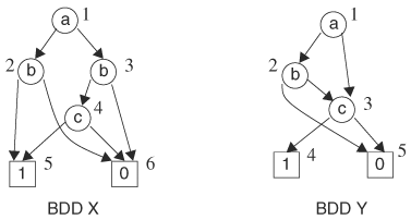

Figure 8.12. Intermediate and final result from BDD ITE operations (A) BDD created by ITE operations (B) Reduced BDD
The ITE algorithm is summarized here:
Boolean Operations on BDDs: ITE(A, B, C)
Input: Three BDDs, A, B, and C.
Output: ROBDD representing ITE(A, B, C).
If ITE(A, B, C) is a terminal case, return with result.
If ITE(A, B, C) is in the computed table, return with result.
Select the root variable x that is ordered earliest.
Compute BDD0 = ITE(
 ,
,  ,
,  ) and BDD1 = ITE(Ax, Bx, Cx).
If (BDD0 = BDD1), return BDD0.
If (x, root of BDD1, root of BDD0) is in the unique table, return the existing node.
Create BDD node x with 0-edge and 1-edge pointing to BDD0 and BDD1 respectively.
So far in our discussion of BDDs, we have assumed an arbitrary variable ordering. Different variable orderings can cause drastic differences in BDD size Example 8.7 dramatizes the effect and sheds some insight into what makes a variable ordering good.

Figure 8.13. Impact of variable ordering on BDD size. (A) BDD with variable ordering a1, a2, b1, b2, c1, c2 (B) BDD with variable ordering a1, b1, c1, a2, b2, c2
The following two observations provide insight into what makes up a good variable ordering. First, the “width” of a BDD, crudely defined as the number of paths from root to the constant nodes, is determined by the “height” of the BDD, which is the average number of variable nodes along paths, because each variable node branches to two paths. Thus, the more nodes there are on a path, the more branches do the nodes produce, and the wider the BDD. The size of a BDD is proportional to the product of the width and height; hence, the height determines the BDD size. Roughly speaking, the larger the average number of variable nodes along the paths, the bigger the BDD size. Now let’s relate variable ordering to the number of variable nodes along paths. The variable nodes on a path represent the minimum knowledge about the variables such that the value of the function is determined. Therefore, the less knowledge required to know about variables to determine the function’s value, the smaller the BDD size. Hence, a good variable ordering should have the property that, as variables are evaluated one by one in the order, the function value is decided with the fewest number of variables the sooner a function’s value is decided, the fewer variable nodes are on the paths.
Second, node sharing reduces BDD size. Let node v be shared by two paths. Let us call the variables ordered before v the predecessors, and the variables ordered after v the successors. The portions of the two paths from the root to v correspond to two sets of values assigned to the predecessors. The fact that the two paths share node v implies that the valuation of the function by variable v and its successors is independent of the two assigned values to the predecessors. Hence, the more independent the successors and predecessors are in a variable ordering, the more sharing that occurs and thus the smaller the resulting BDD. In other words, a good variable ordering groups interdependent variables closer together.
Deriving a variable ordering from circuits also follows these two principles but manifests slightly differently and uses the circuit structure to select the variables. The key is to arrange the variables such that as evaluation proceeds in the order, the function simplifies as quickly as possible and is as much independent of the already assigned values as possible. Many heuristics exist. An example heuristic is to level the gates from the primary output (the level of a gate being the shortest distance to the output and the distance being the number of gates in between) and order the inputs in increasing level number. The rationale is that variables closer to the output have a better chance of deciding the value of the circuit and hence create BDD paths with fewer nodes. In addition, order the primary input variables such that the intermediate node values are determined as soon as possible. The idea lies in the hope that when intermediate node values are determined, the circuit simplifies.
When composing or computing an operation on several Boolean functions, each of which has its own good ordering, a question arises about how to derive a good ordering for the resulting BDD based on the orderings of the operands. A heuristic is to interleave variable orderings to form an initial overall ordering. For example, if operand 1 has variable ordering a, b, c, d, and operand 2 has x, y, z, then an interleaved ordering is a, x, b, y, c, z, d. How variables are interleaved also depends on the specific operators. After an initial overall ordering is obtained, dynamic algorithms can be used throughout the computing process to adjust the variable ordering to minimize the sizes of intermediate BDDs. Dynamic variable ordering is discussed next.
So far, the discussion on ordering assumes that an ordering algorithm calculates an ordering of the variables involved in a Boolean computation beforehand and the ordering is used throughout the computation of the functions. Such an ordering algorithm is called static. When a function f is composed with another function g and the result is then operated with yet another function h, a method based on static ordering would first calculate a variable ordering for the variables in f, g, and h, and then use the ordering throughout these two operations. However, a better strategy is to choose a good variable ordering for each of the operations, as opposed to one ordering for all operations. Even during the process of computing a single operation, oftentimes BDD size varies over the entire computational process and peaks in the middle of the process. Therefore, it is difficult to predict an optimal or good ordering for the entire computing process. In fact, an optimal algorithm may have to change variable ordering during the computing process. A dynamic variable ordering algorithm changes the variable ordering as the BDD size approaches a threshold, and usually makes local and incremental adjustments. A typical application of a dynamic algorithm is to build a BDD with a variable ordering derived from a static algorithm, then use a dynamic algorithm to modify the ordering to improve the BDD size during subsequent computations. A requirement for dynamic algorithms is that they must have minimal computational cost so that their use, instead of finding a new ordering using a static algorithm, is justified.
A simple dynamic ordering algorithm is based on the repetitive application of the swap operation, which exchanges the position of two adjacent variables. Referring to Figure 8.15A, variable x is ordered ahead of y and we want to reverse their order. To swap variable x with y, the labels of the nodes are exchanged and the inner two nodes, b and c, are swapped. This swap operation preserves the functionality of the BDD, because for all possible values of x and y, the same child nodes (a, b, c, d) are reached in each case. For example, x = 1, y = 0 reaches node b before and after the swap. After swapping, a reduce operation may be required to maintain local canonicity, as is the case in Figure 8.15B. Therefore, we conclude that a swap operation has a low computational cost and can be done locally.

Figure 8.15. Swap two adjacent BDD variables. (A) Swap operation. (B) Swap operation followed by a reduce operation.
Any variable ordering can be obtained from an initial ordering through multiple swap operations, and thus, in theory, the optimal ordering can be achieved from an initial ordering using only swap operations. However, in practice, there is no known guidance for selecting variables for swapping for optimal ordering, except for exploring all permutations. Therefore, a greedy algorithm is often used with the swap operation. A sifting algorithm moves a selected variable to all possible positions and chooses the one with the smallest BDD size. For example, suppose the current variable ordering is a < b < c < d < e. Sifting variable d produces the five orderings shown in Table 8.2. In this example, the ordering a < d < b < c < e gives the smallest BDD and thus is kept. Sifting a single variable may be regarded as searching along the variable’s axis. Sifting multiple variables simultaneously explores more space and may produce a better result.
Variable ordering algorithms are only useful for the functions that have a good ordering. There are functions that always have BDD sizes exponential in the number of input variables for any variable ordering. A well-known such function is the multiplication function. Specifically, let x1, ..., xn and y1, ..., yn be the Boolean variables of two multiplicands, and z1, ...,z2n, those of the result—that is, (z2n, ..., z1) = multiply(xn, ... x1, yn, ..., y1). The output functions of 3-bit multiplication are illustrated in Figure 8.16. Variable ci is the carry from output bits before the ith bit. For example, c3 is 1 only if the two product terms in z2 are both 1. In other words, c3 = x1x2y1y2 and z3 = x1y3 + x2y2 + x3y1 + c3. Then, at least one output bit function, zi, has a BDD of size at least 2n/8 for any ordering of x1, ..., xn, y1, ..., yn.

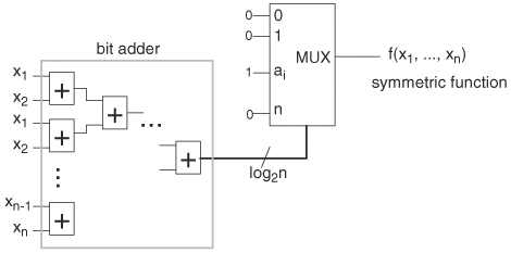
At the other extreme, there are functions with BDDs that are always of polynomial size with respect to any variable ordering. Because symmetric functions are invariant to variable interchanges, their BDD sizes are independent of variable ordering. Recall that a symmetric function is 1 if and only if there is a set of integers, {a1, ..., ak}, such that the number of 1s in the inputs is one of the integers. A symmetric function is completely specified by the set of integers. This fact leads to a universal implementation of symmetric functions. This implementation first adds up all input bits. The result is the number of 1s in the inputs. This result is connected to a multiplexor select line, which selects a 1 if the select value is one of the integers in the symmetric function. Figure 8.17 shows the universal implementation of symmetric function with integer set {a1, ..., ak}. This configuration of adder and multiplexor has a polynomial-size BDD. Therefore, all symmetric functions have polynomial BDD sizes for any ordering.
Unlike these two extreme cases, many functions are sensitive to variable ordering, and their BDDs can change from polynomial size to exponential size and vice versa. A practical and interesting property is how easy it is to find a variable ordering that yields a BDD of reasonable size.
In this section we will study several variants of decision diagrams, all of which are canonical and have efficient manipulation algorithms, such as construction and Boolean operations. Each variant is targeted toward a specific application domain. Therefore, as the application of decision diagrams become more widespread, more variants are sure to come.
Strictly speaking, SBDDs are not a variant of BDDs; rather, they are an application of a BDD to vector Boolean functions. A vector Boolean function has multiple outputs. An example is the next-state function of a finite-state machine having more than one FF. When constructing BDDs for a number of Boolean functions, instead of having a number of isolated BDDs, one for each function, the BDD nodes representing the same functionality are shared. This overall BDD having multiple roots each representing a function is called a shared BDD (or SBDD). The main advantage of an SBDD is compactness through node sharing. An SBDD preserves all the properties of a BDD.
Example 8.9
Construct an SBDD for the following functions:
For illustration purposes let’s first construct a BDD for each function and then merge their nodes. In practice, BDDs for f and g are constructed simultaneously, and node sharing is a part of the construction process. Choose variable ordering a < b < c. To merge nodes of the same functionality, we start from the leaf nodes and move toward the root. The BDDs for f and g and the SBDD are shown in Figure 8.18. The ratio of BDD sizes before and after sharing is 13:9.

It is simple operation to complement a function: by exchanging the constant nodes in the function’s BDD. That is, except for the two constant nodes, the BDD of the function and that of its complement are identical. Being able to share the common structures between the function and its complement can have a drastic effect on overall size, especially for a function with many subfunctions that are complements of each other. One solution to this problem allows BDD edges to carry an attribute that can be an inversion or no inversion. When an edge’s attribute is inversion, the function seen at the tail of the edge is the complement of the function at the head of the edge. To denote an inversion attribute, we place a small dot on the edge.
Allowing unconditional placement of inversion attributes on an edge violates canonicity. For instance, the pairs of BDDs in Figure 8.19 have equivalent functionality, even though they are structurally different. Therefore, we must restrict which edges are allowed to be complemented. For the two equivalent configurations in each pair, we only allow the one with no dot on the 1-edge (in other words, the first configuration). With this restriction, we restore canonicity.


The two reduction rules for BDD are removing nodes with two edges that point to the same node and merging nodes that represent the same functionality. In ZBDDs, the first reduction rule is replaced by removing nodes with a 1-node that is the constant node 0. As illustrated in Figure 8.21, the two transformations for the ZBDD are the following:
Remove the node with a 1-edge that points to constant node 0 and redirect all incoming edges to its 0-node.
Merge nodes that represent the same functionality.

It can be shown that ZBDDs are canonical. However, ZBDD nodes may exist with both edges that point to the same node. Consequently, a ZBDD has the following interpretation. A path from the root to the constant node 1 represents a cube. If a variable is missing in the path, the variable node’s 1-node is constant 0 and therefore the variable is a negative literal in the cube.
Conceptually, a ZBDD can be obtained from a completely unreduced decision diagram by applying the two previous reduction rules. A completely unreduced decision diagram is a graphical representation of the truth table of a function, and hence has exactly 2n paths and 2n leaf nodes, where n is the number of variables, and it can be constructed by applying successive cofactor operations for all variables in the function. Each path represents a minterm, and the value of the leaf node is the value of the function at the minterm. In practice, ZBDDs are not constructed directly from unreduced decision diagrams, but from a procedure that applies the two reduction rules throughout the whole construction process. For more details, please refer to the bibliography.
Example 8.11
Figure 8.22A shows a completely unreduced decision diagram. From this decision diagram, we can apply the ZBDD reduction rules. First, remove all the c nodes with a 1-edge that points to constant node 0, and redirect their incoming edges to their respective 0-nodes, as in Figure 8.22B. Now the left b node has its 1-node as constant 0 and is thus removed, as shown in Figure 8.22C. At this point, node a becomes eligible for removal. Getting rid of node a and sharing the constant node 1, we have a reduced ZBDD in Figure 8.22C. An ROBDD for the same function is shown in Figure 8.23A. Note that the reduced BDD has more nodes and edges. Also note that variable a does not even appear in the ZBDD. Let us try to read the function off the ZBDD. There are two paths to constant node 1. The first path consists of b and c. Because variable a is missing in the path, it is a negative literal in the cube. The cube indicated by the first path is ābc. The second path has only variable b; therefore, the two missing variables show up in the cube as negative literals. This cube is ![]() . The function is the sum of the two cubes:
. The function is the sum of the two cubes: ![]() . The same function can be derived from the BDD.
. The same function can be derived from the BDD.
Not all functions have ZBDDs smaller than BDDs. Apart from sharing nodes, a ZBDD gets reduced in size by removing nodes with 1-edges that point to 0, whereas BDD reduces from removing nodes with both edges that point to the same node. Therefore, a ZBDD has a smaller size than the BDD of the function if there are more such 1-edge-to-0 nodes than the nodes with both edges that point to the same node, and vice versa. A path in a decision diagram represents a cube. Thus, a path having a 1-edge-to-0 node means the cube has a negative phase of the variable. Therefore, intuitively, a ZBDD is more compact if the function to be represented has a lot more negative literals than positive literals in the minterms of its on set. A minterm of n literals can be interpreted as a selection among the n objects: A positive literal at position i means the ith object is selected; a negative literal, the ith object is not selected. Therefore, a function of n variables, expressed as a disjunction of minterms, represents all acceptable selections. A more compact ZBDD results if there are more negative literals, implying that few objects are selected. With this interpretation, sometimes ZBDDs are said to be compact for sparse representation (in other words, the objects selected are sparse).
A BDD is based on the first form of the Shannon cofactoring expansion. It is possible to derive decision diagrams based other expansions. OFDDs are based on positive Davio expansion. Positive and negative Davio expansions are

We will focus our discussion on positive expansion. A function, when expanded with respect to variable x, generates two subfunctions: ![]() and
and ![]() , each of which is independent of x. Expansion continues on the subfunctions until all variables are exhausted. The resulting expansion is called the Reed Muller form, which is an
, each of which is independent of x. Expansion continues on the subfunctions until all variables are exhausted. The resulting expansion is called the Reed Muller form, which is an XOR sum-of-products term. This expansion of a function can be represented graphically, and the resulting graph is called an OFDD. When expanding about variable x, a node labeled x is created and the 1-edge is pointed to the node of the Boolean difference whereas the 0-edge is pointed to the node of the cofactor, as shown in Figure 8.24A. If the cofactor or the Boolean difference is not a constant, the expansion continues.
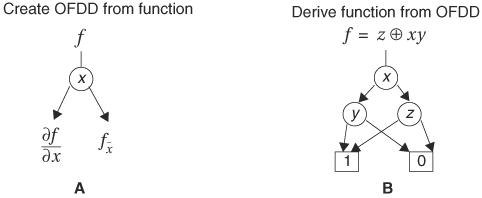
Figure 8.24. OFDD from Davio expansion. (A) Edge semantics of an OFDD node (B) An OFDD for f = z ⊕ xy
Conversely, given an OFDD, the represented function is derived by ANDing the node variable with its 1-node and XORing with its 0-node, as in Figure 8.24B, starting from the leaf nodes and ending at the root. Each path from the root to a leaf node represents a cube. Based on the semantics of an OFDD node, if a path takes the 1-edge of a node, the node variable is included in the cube. If the 0-edge is taken, the variable is not included. Therefore, to obtain a function from an OFDD, enumerate all paths from the root to the constant 1-node. Then generate the cubes for the paths. Finally, XOR all the cubes.
Two reduction rules for OFDDs are the same as those for ZBDDs:
If a node’s 1-edge points to constant 0, remove the node and redirect its incoming edges to its 0-node.
Merge nodes that have the same child nodes.
Rule 1 follows directly the expansion f = g ⊕ xh; if the 1-node is constant 0 (in other words, h = 0, then f = g), meaning that the incoming edges directly point to the 0-node. Rule 2 combines isomorphic nodes.
Example 8.12
Expand the following function using positive Davio expansion and create an OFDD:
Choose variable ordering a < b < c < d.

Now the remaining subfunctions are constants, so we stop. The resulting expansion is as follows and the OFDD is shown in Figure 8.25A:
Now apply the reduction rules to simplify the OFDD. The reduced OFDD is shown in Figure 8.25B. Note that the d node has both edges pointing to the same node, yet the node remains in the OFDD.
As a check, let us derive the Reed Muller form from the OFDD. There are six paths from the root to constant node 1. For each path, the node variable is included in the cube if the path takes the 1-edge of the node. For the path shown Figure 8.25B, because only the 1-edge of node c is taken, the path gives cube c. The other five paths give cubes abc, acd, ac, bc, and bcd. The function is the XORing of the cubes

which is equal to the original function, as expected.

Thus far, the Boolean domain is implied in our study. It is interesting to explore decision diagrams in other domains to see whether advantages such as representation size can be achieved. In this section we will briefly study several decision diagrams for functions that have either or both non-Boolean domain or range. These decision diagrams are extensions from the binary domain to the integer/real domain, and they have found application in specific design and analysis areas.
A generalization of a BDD is to relax the values a variable can take from binary to any set of numbers. Thus, a node can have more than two outgoing edges and each edge is labeled with the value the variable assumes. This decision diagram is called a multivalue decision diagram (MDD). An application of MDDs is to represent a design at an early stage when signals are in symbolic form as opposed to encoded binary form. For instance, the input variables to the function can be control signals with permissible values WAIT, SYNC, ACK, ABORT, ERR, and REQ.
For a multivalue function f: Mk -> M, where M = {1, ..., n} (in other words, f has k variables each of which can have a value between 1 and n), an MDD for f is a DAG with n leaf nodes. The leaf nodes are labeled as 1, ..., n. Each internal node is labeled with a variable and has n outgoing edges. Each edge is labeled with a value between 1 and n. Along any path from the root to a leaf node, a variable is traversed (at most) once. The semantics of an MDD is that a path from the root to a leaf node represents an evaluation of the function. Along the path, if a node takes on value v, the edge labeled v is followed to the next node. When a leaf node labeled i is reached, the function evaluates to i.
An ordered MDD conforms to a variable ordering such that variables along any path are consistent with the ordering. A reduced MDD satisfies the following two conditions: (1) no node exists with all of its outgoing edges pointing to the same node, and (2) no isomorphic subgraphs exist. Like a BDD, a reduced ordered MDD is canonical and has a suite of manipulation operations associated with it. Furthermore, several multivalue functions can be merged and represented as a shared MDD.
Table 8.3. A Multivalue Function f: M3->M
(x,y,z) | f(x,y,z) |
|---|---|
(1, 1, -) | 1 |
(1, 2, z) | z |
(1, 3, -) | 2 |
(2, 1, -) | 1 |
(2, 2, -) | 2 |
(2, 3, z) | z |
(3, -, z) | z |

An algebraic decision diagram (ADD) represents a function with a domain that is Boolean but with a range that is real: f: Bn -> R. An ADD differs from a BDD only in the number of leaf nodes. An ADD has a number of leaf nodes equal to the number of possible output values of the function it represents. A reduced ordered ADD has the same variable ordering and reduction rules as in a BDD. The semantics of ADD nodes are the same as those of BDD nodes. One application of an ADD is in the area of timing analysis. For instance, the function gives the power consumption or delay of a circuit based the circuit input values. Example 8.14 illustrates such an application.
An interesting way to look at Boolean variables is to treat them as integer variables restricted to 0 and 1. TRUTH value is denoted by x and FALSE is denoted by 1 - x. When applying BMD to a function mapping from Bn to R, the inputs to the function can be conveniently expressed as “cubes.” For instance, referring to Table 8.4, the first entry, 000 giving 5, can be expressed as 5(1 − a)(1 −b)(1 − c), which is 5 only if a = b = c = 0 as required. Using this technique and by adding up the “cubes,” a function from Bn to R can be expressed as a polynomial. The function in Example 8.14 has polynomial
A BMD represents the coefficients of the polynomial in leaf nodes. Nonterminal nodes have the interpretation that if the 1-edge (left) is taken, the variable of the node is included; otherwise, the variable is excluded. The path from the root to a leaf node represents a term in the polynomial by multiplying the value of the leaf node and all included variables along the path. Then the function is the sum of the terms represented by all paths. This interpretation is similar to that of OFDDs, which, instead of summation, XORs all cubes. A BMD for the leakage power function is in Figure 8.28. The two paths shown produce the terms ab and -b. The left path takes 1-edge of node a and node b, and 0-edge of node c; thus, variables a and b are included. Furthermore, the leaf node value is 1. Multiplying the variables with the leaf node value gives the term ab. Similarly, the right path takes the 0-edge of node a and node c, and the 1-edge of node b. The leaf node value is -1. Therefore, the term is -b.
The two reduction rules for BMDs are the same as those for OFDDs. That is, first, if the 1-edge of a node points to 0, the node is removed and its incoming edges are redirected to its 0-node. And second, all isomorphic subgraphs are shared. The first rule follows from the multiplicative action of the node variable on the 1-edge. If the 1-edge points to 0, the node variable is zeroed and only the 0-node is left. Therefore, all incoming edges can be redirected to the 0-node. Applying these reduction rules to Figure 8.28A, we obtain the reduced BMD in Figure 8.28B.
A further generalization of BMDs allows edges to carry weight. As a path is traversed, the included variables, the weights on the traversed edges, and the leaf node value are multiplied to produce a term. This generalization gives more freedom to distribute the coefficients, and results in more isomorphic subgraphs for sharing, producing more compact representations. With proper restrictions on subgraph transformations, these generalized BMDs can be reduced to be canonical. For more information, consult the citations in the bibliography.
In this section we will study the use of BDDs in determining the functional equivalence of two Boolean functions or circuits, known as equivalence checking. The ideas presented here are applicable not only to BDDs but also to any canonical decision diagrams. We use BDDs to illustrate the ideas because of their widespread use. A situation in which equivalence checking is called for is when a designer needs to determine whether an RTL description of a circuit is functionally equivalent to its gate-level model or a timing optimized version of the same design. In determining functional equivalence, ROBDDs for the two functions are built and compared structurally. Because of the canonicity of ROBDDs, the two functions are equivalent if and only if their ROBDDs are isomorphic.
Let’s first consider determining the functional equivalence of combinational circuits and then sequential circuits. For combinational circuits, the shared ROBDDs of the outputs of circuits are built and compared. To compare two ROBDDs, one can compare them graphically—that is, map the nodes and edges between the two ROBDDs. We start by identifying the corresponding pairs of ROBDD roots and then follow the edges of the roots. If the 1-node (0-node) of one root is the same variable as the 1-node (0-node) of the other root, the mapping process recurs on the 1-nodes and 0-nodes. Otherwise, a mismatch occurs and the two ROBDDs are not isomorphic. The two ROBDDs are isomorphic if the procedure terminates at the leaf nodes without encountering any mismatched nodes.
Another way to determine whether two shared ROBDDs are isomorphic is to perform an XOR operation on the ROBDDs. If the resulting ROBDD is a constant node 0, the two ROBDDs are isomorphic; otherwise, they are not. This method is also applicable to checking circuit equivalence. To compare two circuits for equivalence, pairs of corresponding outputs are identified. Then these pairs are XOR, and the XOR gate outputs are ORed to produce a single output, as shown in Figure 8.29. If any pair of the outputs is not equivalent, the XOR output of the pair becomes 1, thus producing a 1 at the output of the OR gate. Next, an ROBDD is built for output differ of this overall circuit. Therefore, the circuits are equivalent if the ROBDD is equal to constant node 0. If the ROBDD is not constant 0, any path in the ROBDD from root to constant 1 is an input vector that demonstrates the difference in output response from the two circuits.

Checking the equivalence of sequential circuits is simplified when correspondence of state bits between the two circuits can be identified. For instance, the ith FF in circuit A is identified with the jth FF in circuit B. If such a one-to-one state correspondence is known, equivalence of the two circuits reduces to checking equivalence of the next-state functions, which are combinational circuits. A next-state function has as input the primary inputs and outputs of the FFs, and has as outputs the primary outputs and inputs of the FFs. If a one-to-one mapping between the state bits is not available, the two sequential circuits can be connected, as shown in Figure 8.29. Techniques in model checking are used to search the state space to prove or disprove that output differ is identically equal to 0. We discuss modeling checking in Chapter 9 (see “Equivalence Checking” on page 502).
In practice, it is rare that these methods work outright without modification. The main problems are running out of memory space or runtime taking too long. To mitigate these problems, two common techniques are used. The first technique identifies as many possible pairs of internal or I/O nodes that are required or known to be equivalent. These nodes are called cut points. This can be done through user-defined mapping between pairs of nodes in the two circuits or by assuming that nodes with the same name correspond to each other. Equating nodes with the same name is based on the rationale that one circuit is often a synthesized version or slightly modified version of the other, and therefore most node names are preserved between the two circuits. Once such a mapping is obtained, the mapped nodes are broken so that the fanins to the nodes are considered as outputs, and the fanouts are considered inputs. The two circuits with these newly formed inputs and outputs, together with the original primary inputs and outputs, are checked for equivalence. The advantage of breaking the known equivalent points and creating new inputs and outputs is that, although there are more outputs to check, the BDDs for the outputs have become smaller, as illustrated in Example 8.15.
Example 8.15
Let’s assume we want to check the equivalence of the circuit shown in Figure 8.30A, which is a gate-level model and the RTL model of the same circuit in Figure 8.30B. The first method simply builds ROBDDs for the two circuits and compares the BDDs. The second method identifies three cut points—namely x, y, and z in the gate-level model and x’, y’, and z’ in the RTL model. That is, node x should be functionally equivalent to node x’, y to y’, and z to z’. This knowledge can be supplied by the designer. In this example, let’s compare the largest BDD sizes in the two methods. For simplicity, we will use only the BDDs of the gate-level model in this exercise.
With the first method there is only one output, f, and five inputs: a, b, c, d, and e. So two BDDs are built, one for the gate model and the other for the RTL model. The BDD for the gate model is shown in Figure 8.31A, which has 13 nodes.
With the second method, the three pairs of internal nodes are identified to be equivalent and the cut points are x, y, and z. We then cut the circuit at these points and create three inputs and outputs, as shown in Figure 8.32. Now, instead of just one BDD, we have to construct four BDDs for the four outputs f, x, y, and z. Then we construct ROBDDs for the four pairs of nodes—(x,x’), (y,y’), (z,z’), and (f,f’)—and compare the respective BDD pairs. If any one of these BDD pairs is not equivalent, the circuits are not equivalent. In practice, if these BDD pairs are not equivalent, the first thing the designer needs to do is to reexamine the assumption that these internal node pairs are indeed equivalent. The BDDs for the internal nodes are shown in Figures 8.31B, C, and D. Because the internal nodes are also inputs, output f can be expressed in terms of the internal nodes (![]() ), the BDD of which is shown in Figure 8.31E. The largest BDD size of the second method is the BDD size of node x, which has eight nodes. As illustrated in this example, we can see that the largest BDD size has been reduced greatly by using cut points.
), the BDD of which is shown in Figure 8.31E. The largest BDD size of the second method is the BDD size of node x, which has eight nodes. As illustrated in this example, we can see that the largest BDD size has been reduced greatly by using cut points.
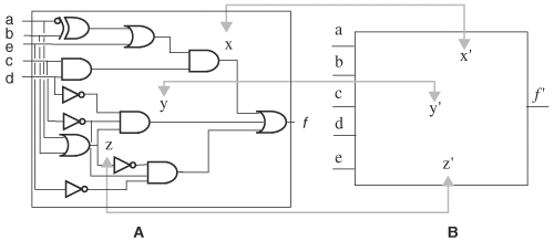

Figure 8.31. Compare the largest BDD sizes with and without node mapping. (A) BDD for node f (B) BDD for node x (C) BDD for node y (D) BDD for node z (E) BDD for node f in terms of new variables

Thus far, we have assumed that the inputs of the circuits undergoing equivalence checking are unconstrained (that is, the inputs can take on any values). When two circuits are equivalent only in a restricted input or state space, then the input or state space must be constrained. An example of equivalence under restricted space is comparing the next-state function of two finite-state machines. To perform equivalence checking in this situation, the FFs are removed and the next-state functions are compared as stand-alone combinational circuits. Because the next-state functions are now stand-alone functions, their inputs can take on any value. If the finite-state machines do not reach the entire state space, then the inputs to the next-state function must be constrained to the reachable state space of the finite-state machines; otherwise, it is possible that the next-state functions are not equivalent outside the reachable state space. Constraining eliminates the unreachable portion of search space from giving a false negative. Besides limiting input space, constraining can also restrict the structure of a circuit for equivalence checking (for example, by deactivating the scanning portion of a circuit by setting the scan mode to false). The following are some common applications for which constraining plays an important role:
Compare next-state functions. Constrain the state space to be the reachable state space of the finite-state machines.
Compare prescan and postscan circuits. Constrain to eliminate the scan logic so that only the main logic portions of the circuits are checked.
Reduce runtime and memory use. Constrain the input search space so that an equivalence checking operation finishes within a specific time and space limit.
Compare a unit of two circuits. Constrain the peripheral circuitry surrounding the unit so that the environment of the unit is the same as that inside the circuit. This is a more general situation than the reachable state space constraining method mentioned earlier. Figure 8.33 shows the problem and the idea of input constraining, where the constraining function maps the entire input space to the smaller realizable input space that unit A expects to see when embedded within the original circuit.
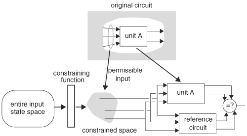
Constraining can be done directly by mapping an unconstrained input space into a permissible input space, as illustrated in Figure 8.33, or indirectly by creating an exclusion function that defaults the two circuits to be equivalent when it detects an input that lies outside the permissible region, as illustrated in Figure 8.34. The entire input space, permission and forbidden, is applied to the circuits under comparison. The exclusion function outputs 1 when an input is forbidden, which then forces the comparison to be equal. Therefore, for the output of this comparison structure always to be 1, the circuits must be equivalent. This indirect method of constraining is easy to implement, as illustrated in Example 8.16.

Example 8.16
Suppose that a finite-state machine never reaches states 1001 and 1100. Let a, b, c, and d be the state bits. To check equivalence of this machine’s next-state function, we can either prevent these two states from being fed to the comparison structure or allow them to be input, but force the result to be equal. Let’s choose the latter. To exclude these two states, we define an exclusion function to be ![]() . If f and h are the outputs of the next-state function and a reference circuit, respectively, the output of the comparison structure is
. If f and h are the outputs of the next-state function and a reference circuit, respectively, the output of the comparison structure is ![]() . If f and h are not equivalent, there exists an input in the permissible region, g = 0, such that
. If f and h are not equivalent, there exists an input in the permissible region, g = 0, such that ![]() , and hence d = 0. Therefore, output d is always 1 if and only if f and h are equivalent. So, we build a BDD for d and determine whether this BDD reduces to the constant 1.
, and hence d = 0. Therefore, output d is always 1 if and only if f and h are equivalent. So, we build a BDD for d and determine whether this BDD reduces to the constant 1.
An alternative to BDDs in checking equivalence uses techniques from determining Boolean satisfiability called SAT. The problem of Boolean satisfiability decides whether a Boolean expression or formula is identically equal to 1. That is, it is satisfiable if there is an assignment to the variables of the expression such that the expression evaluates to 1. Equivalence checking is translated into the SAT problem by XORing the two functions: d = f ⊕ g. If expression d is satisfiable, then f is not equivalent to g. Otherwise, f is equivalent to g. The expression in Boolean satisfiability is in a conjunctive form—the product of sums. A sum is called a clause. If each clause of the conjunctive form has at most two variables, then the problem of Boolean satisfiability is called 2-SAT. Similarly, if each clause has at most three variables, it is called 3-SAT. 2-SAT can be solved in polynomial time, whereas 3-SAT is NP complete. Furthermore, satisfiability of any Boolean expression can be polynomially reduced to 3-SAT. In other words, if 3-SAT can be solved in polynomial time, so can any SAT problem. Hence, in the following discussion, we will not distinguish 3-SAT from a general SAT problem. We will just use the term SAT.
Example 8.17
Determine whether the following expression is satisfiable:
For this expression to evaluate to 1, all clauses must evaluate to 1 for some variable assignment. Let us solve this problem by trial and error. Variable assignment a = 1 makes the first clause 1, b = 1 makes the second clause 1, and c = 0 makes the fourth clause 1, but the fifth clause evaluates to 0. Try again. Pick a = 1 and c = 0 to make the first four clauses 1. The last clause is 1 if b = 0. Thus, for variable assignment a = 1, b = 0, c = 0, the expression is satisfied. In the worst case, we may have to try all 23 (or eight) variable assignments to reach the conclusion.
In the following discussion, we will look at two classes of algorithms to solve SAT problems. We will first discuss a mathematically elegant method (a resolvent method) and then a more efficient method based on search.
This method is based on the following resolvent and consensus identity:
and
where A and B are sums of literals, and C and D are product of literals. A + B is called the resolvent of (x + A) and (![]() ). CD is called the consensus of xC and
). CD is called the consensus of xC and ![]() . The resolvent identity is applicable to the conjunctive form whereas the consensus identity is applicable to the disjunctive form. In the following discussion we will use the resolvent identity on conjunctive forms.
. The resolvent identity is applicable to the conjunctive form whereas the consensus identity is applicable to the disjunctive form. In the following discussion we will use the resolvent identity on conjunctive forms.
Now, we want to show that A + B is satisfiable if and only if (x + A)(![]() ) is satisfiable. According to the resolvent identity, if A + B is satisfiable, then A, B, or both is satisfiable. Let us assume A is satisfiable. Then, when x = 0, (x + A)(
) is satisfiable. According to the resolvent identity, if A + B is satisfiable, then A, B, or both is satisfiable. Let us assume A is satisfiable. Then, when x = 0, (x + A)(![]() ) becomes A and thus is satisfiable. Similarly, if B is satisfiable, then when x = 1, (x + A)(
) becomes A and thus is satisfiable. Similarly, if B is satisfiable, then when x = 1, (x + A)(![]() ) become B and thus is satisfiable. On the other hand, if (x + A)(
) become B and thus is satisfiable. On the other hand, if (x + A)(![]() ) is satisfiable, then (x + A)(
) is satisfiable, then (x + A)(![]() ) is satisfiable when x = 0 or x = 1. Let us consider both cases. At x = 0, (x + A)(
) is satisfiable when x = 0 or x = 1. Let us consider both cases. At x = 0, (x + A)(![]() ) becomes A and therefore A must be satisfiable. At x = 1, (x + A)(
) becomes A and therefore A must be satisfiable. At x = 1, (x + A)(![]() ) becomes B and hence B must be satisfiable. Therefore, either A or B must be satisfiable if (x + A)(
) becomes B and hence B must be satisfiable. Therefore, either A or B must be satisfiable if (x + A)(![]() ) is satisfiable. In conclusion, (x + A)(
) is satisfiable. In conclusion, (x + A)(![]() ) is satisfiable if and only if A + B is satisfiable. Note that the variable assignments satisfying A + B do not necessarily satisfy (x + A)(
) is satisfiable if and only if A + B is satisfiable. Note that the variable assignments satisfying A + B do not necessarily satisfy (x + A)(![]() ). For a counterexample, see Example 8.18 on page 433. By translating the satisfiability problem of (x + A)(
). For a counterexample, see Example 8.18 on page 433. By translating the satisfiability problem of (x + A)(![]() ) to that of A + B, the problem complexity is reduced by one variable—namely, variable x. Extending from two clauses to more clauses, consider (x + A)(
) to that of A + B, the problem complexity is reduced by one variable—namely, variable x. Extending from two clauses to more clauses, consider (x + A)(![]() ) (x + C)(
) (x + C)(![]() ). We form the resolvent for all pairs of clauses containing both phases of x. There are a total of four pairs: (x + A)(
). We form the resolvent for all pairs of clauses containing both phases of x. There are a total of four pairs: (x + A)(![]() ), (x + A)(
), (x + A)(![]() ), (x + C)(
), (x + C)(![]() ), and (x + C)(
), and (x + C)(![]() ). For each pair, we obtain its resolvent. Combining all resolvents, we conclude that (x + A)(
). For each pair, we obtain its resolvent. Combining all resolvents, we conclude that (x + A)(![]() )(x + C)(
)(x + C)(![]() ) is satisfiable if and only if (A + B)(A + D)(C + B) (C + D) is satisfiable. Replacing clauses containing variable x or
) is satisfiable if and only if (A + B)(A + D)(C + B) (C + D) is satisfiable. Replacing clauses containing variable x or ![]() by their resolvents is called resolving variable x.
by their resolvents is called resolving variable x.
After a variable has been resolved, there are straightforward cases that other variable assignments can be easily inferred. If these straightforward cases exist, as many as possible variable assignments are inferred before resolving another variable. Here we will examine some of straightforward cases. First, if a resolvent contains both phases of a variable, such as the resolvent ![]() in resolving (x + y)(
in resolving (x + y)(![]() ), then the resolvent, being 1, is removed.
), then the resolvent, being 1, is removed.
If both phases of a variable are in a formula, the variable is called binate. If only one phase of the variable appears in the formula, the variable is unate. For example, in ![]() , a is unate, and b and c are binate. For a unate variable, we simply assign the variable to a value so that the clauses having the variable become 1. Consequently, the resulting formula formed by replacing the clauses containing the unate variable with 1 is satisfiable if and only if the original formula is satisfiable. This replacement operation is called the unate variable rule or the pure literal rule. Therefore, only binate variables need to be resolved.
, a is unate, and b and c are binate. For a unate variable, we simply assign the variable to a value so that the clauses having the variable become 1. Consequently, the resulting formula formed by replacing the clauses containing the unate variable with 1 is satisfiable if and only if the original formula is satisfiable. This replacement operation is called the unate variable rule or the pure literal rule. Therefore, only binate variables need to be resolved.
Another straightforward case is when a clause contains only one literal. For instance, in (a + b + c)(![]() )(
)(![]() ), the second clause contains only one literal,
), the second clause contains only one literal, ![]() . Then the variable must be assigned to the value at which the clause is satisfied, which is b = 0 in this case. This rule is called the unit clause rule and the literal in the clause is called the unit literal.
. Then the variable must be assigned to the value at which the clause is satisfied, which is b = 0 in this case. This rule is called the unit clause rule and the literal in the clause is called the unit literal.
We define an empty clause to be a clause that contains no literals. The resolvent of (x)(![]() ) is an empty clause. A formula containing an empty clause is unsatisfiable. With this definition, the resolvent algorithm is as follows:
) is an empty clause. A formula containing an empty clause is unsatisfiable. With this definition, the resolvent algorithm is as follows:
Example 8.18
Let us use the resolvent algorithm to determine the satisfiability of
Select variable a for resolution. For each pair of clauses containing both phases of a, form its resolvent. Clause pairs and their resolvents are shown in Table 8.5. The first column lists the clause pairs containing both phases of a. The second column is the resolvents. The third column is the simplified resolvents. Therefore,
is satisfiable if and only if ![]() is satisfiable. Because both variables, b and c, are unate, we apply the unate rule. So
is satisfiable. Because both variables, b and c, are unate, we apply the unate rule. So ![]() reduces to 1. Therefore, the original expression is satisfiable.
reduces to 1. Therefore, the original expression is satisfiable.
Note that the resolvent algorithm does not imply that variable assignments satisfying ![]() also satisfy the original expression. As a simple counterexample, a = b = c = 0 satisfies
also satisfy the original expression. As a simple counterexample, a = b = c = 0 satisfies ![]() , but does not satisfy the original expression.
, but does not satisfy the original expression.
Table 8.5. Binate Clauses and Resolvents
Binate Clauses | Resolvent | Simplifies To |
|---|---|---|
a + b + c, |
| 1 |
a + b + c, |
| 1 |
a + b + c, |
| 1 |
|
| 1 |
|
|
|
|
| 1 |
As demonstrated by Example 8.18, a resolvent is produced for every pair of clauses containing both phases of a variable. In the worst case, an exponential number of resolvents is computed in solving a SAT problem. Therefore, although mathematically elegant, the resolvent algorithm is reserved for small SAT problems. To deal with large problems, a more efficient search algorithm is required.
A search-based algorithm enumerates all input assignments and evaluates them to decide whether a formula is satisfiable. The set of all possible assignments of the variables in a formula forms the search space. The search space can be represented by a binary tree. A node in the tree represents a variable and has two edges. The left edge represents the variable taking value 1; and the right edge, value 0. A path from the root to a leaf node is a variable assignment, and the value of the leaf node is the value of the formula under the variable assignment. There are a total of 2n leaf nodes for n variables. A partial path gives a partial variable assignment. If the value of the formula evaluates to 1 at a leaf node, the formula is satisfiable. Therefore, a formula is satisfiable if there is a leaf node of value 1.
Although, in the worst case, a search-based algorithm has to traverse the entire binary tree, oftentimes pruning techniques are used to cut down the number of paths with values that can be deduced. Figure 8.35 illustrates the concept of the search strategy and pruning technique. Suppose we start the search following path P1. Path P1 is a variable assignment of a = 0, c = 1, d = 1, and b = 1. The leaf node for the path is 0. Thus, for this variable assignment, the formula is not satisfied. Let’s backtrack to the last decision node b and take the other choice, b = 0. Backtracking to a previous decision variable and selecting the other value for the variable is called flipping the variable. With this new assignment, the formula is satisfied. In general, backtracking does not have to return to the last decision node; it can return to any prior decision node (for example, decision node c).

Next let’s consider a situation in which pruning eliminates the necessity of visiting all paths. Partial path P2 represents the partial variable assignment a = 1, b = 1. Note that the all leaf nodes following this partial path have value 0, meaning that the formula cannot be satisfied if a = 1 and b = 1. Therefore, no further assignments need to be considered; that is, the tree rooted at the c node can be pruned. An intelligent pruning algorithm has to detect this type of subtree at the earliest time.
A search-based SAT solver finds a satisfying variable assignment by making one variable assignment at a time. The candidate variable for assignment is selected based on some heuristic that determines the variable with the “best” chance of making the formula satisfied. Then, after the assignment of the variable is done, the solver attempts to infer as many possible assignments to other variables that must be made to satisfy the formula. After the variable assignment and consequent inferred assignments are made, the formula is evaluated for the partial assignment and is simplified. For example, if x in ![]() is selected and assigned 0, the SAT solver substitutes 0 into x and evaluates it to be
is selected and assigned 0, the SAT solver substitutes 0 into x and evaluates it to be ![]() .
.
During the evaluation process, three cases are possible for a clause: First, the clause is resolved (evaluates to 1); second, the clause is conflicted (evaluates to 0); and third, the clause does not evaluate to a constant (is indeterminate). If the result of an evaluation of the formula turns out to be 0 and there are still unenumerated variable assignments, some prior variable assignments must be reversed; that is, the solver needs to backtrack. For the other two cases, the search continues. If an evaluation produces a result of 1 for the formula, the formula is satisfiable. On the other hand, if all assignments produce a result of 0, the formula is unsatisfiable.
An efficient search-based algorithm should not enumerate all assignments one by one, but should prune as many assignments as possible that would not satisfy the formula. An outline of the structure of a generic search-based algorithm is shown here. Almost all search-based SAT solvers follow this algorithmic structure and differ in the implementation specifics in routines select_branch() and backtrack(). Routine infer() deduces variable assignments based on the partial assignment made so far, and consists of a collection of special cases that imply other variable assignments:
Routine select_branch() selects a variable that has not yet been assigned, called a free variable, and assigns a value to it. Besides, this routine keeps track of previously visited paths and prunes paths based on the values of already assigned variables. If all assignments have been enumerated, it returns a state EXHAUSTED, which means the formula is unsatisfiable. To select a variable that may satisfy the formula as early as possible, select_branch() relies on some measure of predicting the quality of a new variable assignment. An assignment to a variable is of good quality if the assignment has a high probability of being part of a satisfying assignment or reveals that many paths can be pruned. A reliable quality measure is essential to the performance of a SAT solver. In addition to prediction accuracy, a good assignment quality measure must be easy to compute so that it does not become the bottleneck of the solver. Many heuristics exist for measuring assignment quality. An example predictive measure is the number of literals of a variable in the remaining unsatisfied clauses, the rationale being that an assignment to such a variable will satisfy most clauses. Using this quality measure, select_branch() returns an assignment to the variable that satisfies most remaining clauses. For example, if the remaining clauses of a formula are ![]() , then variable b assigned to 1 satisfies three clauses, whereas other variables satisfy fewer clauses. Therefore,
, then variable b assigned to 1 satisfies three clauses, whereas other variables satisfy fewer clauses. Therefore, select_branch() selects variable b and assigns 1 to it.
Routine infer() looks for special cases in the formula that imply immediate assignments for the remaining unassigned variables. These special cases are the same as those discussed in our study of resolvent algorithms: pure literal rule and unit clause rule. In the pure literal case, there is a variable that appears in only one phase in the formula. The assignment for the variable is then inferred such that the literal becomes 1. For example, a negative-phase literal ![]() implies x = 0. In the unit clause case, there is a clause that contains only one literal, so the literal is assigned to 1. The inferred assignments are then substituted into the formula, and the satisfied clauses are removed. This propagation of assignments is called Boolean constraint propagation (BCP). An important requirement in implementing BCP is that it must save a history of previous assignments so that, at the request of routine
implies x = 0. In the unit clause case, there is a clause that contains only one literal, so the literal is assigned to 1. The inferred assignments are then substituted into the formula, and the satisfied clauses are removed. This propagation of assignments is called Boolean constraint propagation (BCP). An important requirement in implementing BCP is that it must save a history of previous assignments so that, at the request of routine backtrack(), it can return a previously unassigned value. As an example of the operation of infer(), suppose that the current partial assignment is a = 0, b = 1 in satisfying ![]() . After BCP, the formula becomes (
. After BCP, the formula becomes (![]() )(c + d). Hence it can be inferred that the first clause being a unit clause, c = 0. After a BCP for c = 0, it infers from the second clause that d = 1. In this case, the result is SAT. If the result of
)(c + d). Hence it can be inferred that the first clause being a unit clause, c = 0. After a BCP for c = 0, it infers from the second clause that d = 1. In this case, the result is SAT. If the result of infer() is SAT, the formula is satisfiable. If the result is UNSAT, it has to backtrack to a prior decision.
When a partial assignment fails to satisfy the formula, some of the previous assignments must be reversed. Determining the variables to reverse their values is the task for routine backtrack(). Many heuristics exist for selecting variables. The simplest one is to flip the most recently assigned free variable selected by select_branch() that has not been flipped. Note that a variable most recently assigned by infer() must not be chosen for flipping, because such an assignment was forced by another assignment. Therefore, a candidate variable for flipping must be a variable that was assigned by select_branch(). This strategy of reversing the last decision is called chronological backtracking. On the other hand, nonchronological backtracking, when choosing variables to be flipped, does not necessarily flip the last decision variable. It first analyzes the reasons for a conflict, determines the variable assignments that are probable causes of the conflict, and then reverses the root, causing assignment.
If the current partial assignment is not sufficient to determine satisfiability of the formula, the result from infer() is UNDETERMINATE, and it calls select_branch() for the next branch.
Example 8.19
Determine satisfiability of the following formula:
With the select_branch() routine, we use the heuristic that chooses the literal with the highest count. In the formula, ![]() and a each appear four times. To break the tie, let’s arbitrarily select
and a each appear four times. To break the tie, let’s arbitrarily select ![]() . Propagating d = 0 into the formula, we obtain
. Propagating d = 0 into the formula, we obtain
Now literals a and ![]() have the highest count of three each. Arbitrarily selecting a and propagating a = 1, we get
have the highest count of three each. Arbitrarily selecting a and propagating a = 1, we get ![]() .
.
From this, the first two clauses are unit clauses. So, we infer that b must be 1 and c must be 0. However, when we apply BCP to this expression, it becomes 0. Therefore, we backtrack chronologically to the last decision, a = 1. Reversing the decision, we assign 0 to a. Propagating this assignment to ![]() , we get
, we get ![]() .
.
We infer that b must be 1. After applying the unit clause rule to remove literal b, we have (c)(ē + f), from which we further infer that c must be 1. Again, using the unit clause rule to remove literal c, we arrive at (ē + f), to which we apply the pure literal rule to deduce e = 0, and conclude that the formula has been satisfied. Therefore, the formula is satisfiable and a satisfying assignment is d = 0, a = 0, b = 1, c = 1, and e = 0.
When an assignment is searched to satisfy a formula, some free variables are selected to take on certain values. The values form a branch in the decision diagram. The selected variables are called decision variables. If the assigned values cause a conflict, other values are assigned. When a decision variable is selected, we associate a decision-level number with it. The decision-level number keeps track of how deep the assignment is from the top of the search and it facilitates backtracking. Variables with values that are forced by the current decision variable, called implied variables, are consequences of the decision variables and are thus assigned the current decision-level number. The decision number starts with 1 when the first decision variable is selected.
To facilitate backtracking, we need to understand the causes of the conflict. The cause of a conflict is an assignment of decision variables that eventually leads to the conflict. To express causes of conflicts, implication graphs are useful. An implication graph is a DAG with vertices that represent assignments to variables and edges that represent consequences of variable assignments. A vertex is labeled with the variable name along with its decision level and is assigned a value. A conflict occurs if both 1 and 0 are in the implication graph. The variable of the conflicting vertices is the conflicting variable. Vertices without incident edges are decision variables, because they are not implied by values of other variables.
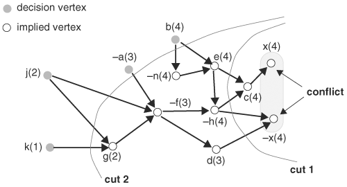
With an implication graph defined, some concepts of an implication graph must be discussed. Vertex v is said to dominate vertex u if any path from a decision variable at the decision level of v to u has to go through v. Intuitively, vertex v determines vertex u. For example, in Figure 8.36, vertex e dominates vertices c and h, because any path from decision vertex b to vertices c or h has to go through e. A unique implication point (UIP) is a vertex at the current decision level that dominates both vertices of a conflict. For example, the vertices of conflict are x(4) and −x(4), and vertex e(4) dominates these vertices; therefore, e(4) is a UIP. The concept of a UIP is used to identify variables to be reversed to resolve a conflict.
When a conflict exists, a cause of the conflict can be obtained by forming a cut on the implication graph such that the graph is partitioned into two parts: reason and conflict. The conflict part contains the conflicting vertices and possibly other implied variables. Note that there is no decision variable in the conflict part. The other part is called the reason part and it consists of all other vertices. Two cuts are shown in Figure 8.36.
The decision variables in the reason part that have an edge to the conflict part contribute to a cause of the conflict. The edges of decision variables crossing a cut represent assignments leading to the conflict and hence must be avoided.
When a search encounters a conflict, the path leading to the conflict should be avoided in any future search. This path of conflict can be learned by including a clause in the formula so that this particular variable assignment can be avoided early during the search. To do so, a cut of a conflict is first determined. Then, the edges of the decision variables crossing the cut are identified. These edges form a clause, which when satisfied avoids the conflict, resulting in an assignment. For example, cut 1 in Figure 8.36 corresponds to variable assignment e = 1, h = 0, d = 1, which results in a conflict. To avoid this partial assignment, any future assignment must satisfy one of the following: e = 0 or h = 1, or d = 0. In other words, clause ![]() must be satisfied. This new clause can be added to the original formula. Note that the added clause is redundant in the sense that it does not change the satisfiability of the formula. Its only function is to speed up decision making by preventing a repeat of known conflicting assignments.
must be satisfied. This new clause can be added to the original formula. Note that the added clause is redundant in the sense that it does not change the satisfiability of the formula. Its only function is to speed up decision making by preventing a repeat of known conflicting assignments.
There can be more than one cut per conflict. Different cuts give different learning clauses. A preferred cut is one that contains only one decision variable assigned at the current level and others assigned at lower levels, because this is the variable that has the most immediate impact on the conflict, and its value should be reversed in backtracking. Cuts with this property are called asserting cuts. At a given decision level, an asserting cut can always be found because the decision variable at the current level is always a UIP. Different cuts represent different learning schemes. For more in-depth information, consult the bibliography.
Example 8.21
Consider the satisfiability of
To satisfy the formula, variable e must be assigned 1. Because there is no decision variable chosen yet, variable e has decision level 0. At level 1, we choose variable a as a decision variable and assign it to 1. This selection reduces the formula to
which implies that variable c must be 0. Thus, the formula further simplifies to ![]() . The next decision variable selected is b. Suppose we assign it to 1. This assignment forces variable d in the first clause to be 0, and variable d in the second clause to be 1—a conflict. An implication graph for the process so far is shown in Figure 8.37. The cut shown gives clause
. The next decision variable selected is b. Suppose we assign it to 1. This assignment forces variable d in the first clause to be 0, and variable d in the second clause to be 1—a conflict. An implication graph for the process so far is shown in Figure 8.37. The cut shown gives clause ![]() which is
which is ANDed with the original formula to prevent future decisions from arriving at this conflict. Therefore, the formula with this learned clause is
Now we can either decide this formula or backtrack. To continue the decision process, we infer that c = 0, which implies (through the learned clause) b = 0. This assignment satisfies the formula. If we backtrack, we first find a cut. The cut shown is an asserting cut, and the variable to flip is b. Assigning b to 0 satisfies the formula.

With traditional simulation, stimuli as well as responses consist of bits of binary constants. In a combinational circuit with n input bits, the input space has 2n vectors, or points. A traditional simulator simulates one point at a time. On the contrary, symbolic simulation takes in variables, called free variables, as input and produces output expressions in terms of the variables. An input at each cycle is a free variable. Because a variable represents both 0 and 1, a symbolic simulator simulates simultaneously the entire set of the points that the input variables can take on. With traditional simulation, constants 0 and 1 are sufficient to represent the simulation values at any time, whereas (because a set of points is computed) a symbolic simulator uses functions to represent sets of points. The functions in a symbolic simulator can be represented using BDDs.
Example 8.22
Simulate the circuit in Figure 8.38 using traditional and symbolic simulation for two cycles. For traditional simulation, assume the input vector sequence is (abcd) = (0011) at cycle 1 and (1101) at cycle 2 and the initial state of the FF is 0. Now do the following: (1) compare the output values at the end of cycle 2 and (2) prove or disprove the property that output f can remain at value 1 for two cycles.
First, we will simulate using the traditional simulation methodology. At cycle 1, the values at nodes h, g, k, n, j, and f are 1, 0, 0, 0, 1, and 1 respectively. At cycle 2, the values at nodes h, g, k, n, j, and f are 0, 0, 1, 1, 1, and 0 respectively.
With symbolic simulation, symbolic values are used at nodes and each cycle has its own free variables. Let’s use subscript labeling to denote time for a symbol. For instance, for input a, a1 denotes the symbol at input a at cycle 1; and a2, the symbol at cycle 2. Let’s assume that the initial value of the FF is k1.
At cycle 1 the symbolic value for node h is computed by NORing the inputs, giving ![]() ; at node g, the value is b1 · c1; at node k, the value is k1. Thus, the value at node f is
; at node g, the value is b1 · c1; at node k, the value is k1. Thus, the value at node f is ![]() . The values of nodes n and j are
. The values of nodes n and j are ![]() and
and ![]() respectively. These values are listed in Table 8.6. Variables a1, b1, c1, d1, and k1 are independent of each other (in other words, they are free variables).
respectively. These values are listed in Table 8.6. Variables a1, b1, c1, d1, and k1 are independent of each other (in other words, they are free variables).
Similar computations are done for cycle 2. k2 = j1 and f2 is ![]() . To express this result in terms of the inputs, we simply substitute the expressions for k2, h2, and g2. The results are tabulated in Table 8.7. Again, a1, b1, c1, d1, k1, a2, b2, c2, and d2 are free variables.
. To express this result in terms of the inputs, we simply substitute the expressions for k2, h2, and g2. The results are tabulated in Table 8.7. Again, a1, b1, c1, d1, k1, a2, b2, c2, and d2 are free variables.
To compare this with traditional simulation for the given input vectors, we need to substitute the input values and compute the output at cycles 1 and 2. For the first input vector (0011), we have a1 = 0, b1 = 0, c1 = 1, and d1 = 1. For the second input vector (1101), a2 = 1, b2 = 1, c2 = 0, and d2 = 1. The initial value of the FF is 0, k1 = 0. Evaluating the expressions for f1 and f2, we have f1 = 1 and f2 = 0, as expected.
For part 2, because f = 1 at cycle 1, if we can show f = 1 at cycle 2, the property is affirmed. With traditional simulation this is difficult to determine without simulating other input vectors, and it is not obvious which input vectors can produce f to be 1 at cycle 2. With symbolic simulation, we just need to check whether f2 is satisfiable under the constraint that a1 = 0, b1 = 0, c1 = 1, d1 = 1, and k1 = 0. To do this, we substitute in the constraint a1 = 0, b1 = 0, into f2 and it simplifies to b2 · c2, which becomes 1 when b2 = 1 and c2 = 1. Therefore, it is possible for output f to remain at 1 for two cycles.

From the previous example, we see that verifying properties can be achieved easier using symbolic simulation than traditional simulation. This advantage comes directly from the fact that many vectors are simulated at once. However, on the negative side, the complexity of symbolic values grows rapidly as the number of cycles increases, resulting in massive memory use and computational time, thus limiting simulation capacity. Furthermore, note that the nodes with a high-complexity growth rate are the ones that keep track of the history of simulation (in other words, in feedback loops).
Because node values are in symbolic form, the concept of transition and event is no longer as precisely defined as in traditional simulation; therefore, symbolic simulation is mainly used in functional verification as opposed to timing verification. However, an event-driven simulator and a symbolic simulator can couple together to verify both functional and timing properties. In addition, even in functional verification, a traditional cycle-based simulator and a symbolic simulator can team up to verify long tests. The cycle-based simulator runs the initial portions of the tests, leading to the crucial intervals for the properties under verification, and lets the symbolic simulator take over verification during the intervals. Using this methodology, the high complexity from symbolic simulation over the long tests can be avoided.
Symbolical simulation of a circuit for n cycles can be regarded as unrolling the circuit n times. The unrolled circuit is a combinational circuit, and the ith copy of the circuit represents the circuit at cycle i. Thus, the unrolled circuit contains all the symbolic results from the n cycles. Figure 8.39B, which illustrates this unrolling representation, is a three-cycle unrolled combinational circuit of the sequential circuit in Figure 8.39A, equivalent to three cycles of symbolic simulation. Each signal generates a copy for each cycle. For example, x becomes x1, x2, and x3 for the three cycles. In the unrolled circuit, the FF model is a combinational circuit representing the current state s as a function of its previous state and the input r. For DFF, the output is a copy of the input, and is modeled by a wire connecting the input r to the current state s. An unrolled circuit for two cycles of symbolic simulation of the circuit in Figure 8.38 is shown in Figure 8.40. The inputs to this unrolled circuit are the primary inputs at each cycle and the initial state. Figure 8.40 reveals that symbolically simulating one cycle is tantamount to replicating the original circuit once. This is the cause of the rapid growth in complexity.

Figure 8.39. Conceptual representation of symbolic simulation. (A) Original circuit (B) Unrolled circuit representing three cycles of symbolic simulation

The ability to simulate multiple inputs simultaneously allows one to verify conclusively and efficiently some properties or assertions that a traditional simulation methodology would have to enumerate explicitly for all possibilities. The properties, sometimes called assertions, are in the form of Boolean functions of states, internal variables, and external inputs. An example property is that if signal A is high then B must be low after, at most, two cycles.
A property or assertion can be categorized as bound or unbound. A bound property is defined over a finite time interval or a bound number of cycles; otherwise, it is an unbound property. An example of a bound property is that from cycle n to cycle m, at least one packet must arrive. The interval in which this property is defined is from cycle n to m. An example of an unbound property is that after a request has become active, the grant will become active eventually.
To verify a bound property, the circuit can be simulated symbolically for the interval of the property. If the property holds within the interval, the property is affirmed. Suppose that a property is f(x, y, z) = 1 from cycle 5 to cycle 6, where x, y, and z are nodes of a circuit. If f(x5, y5, z5) · f(x6, y6, z6) = 1, where x5, y5, z5, x6, y6, and z6 are results at cycles 5 and 6 from a symbolic simulation, then the property is affirmed.
An unbound property, sometimes called an invariant, is verified if it can be shown that the property holds for all possible inputs and states. A standard verification strategy is to apply mathematical induction on the cycle number: If the invariant holds at the initial cycle and at the nth cycle, given that it holds at the n – 1 cycle, then it holds for all cycles. However, not all invariants are easy to recast into a form amicable for mathematical induction.
Variable constraining restricts some free variables, which can take on any value when unconstrained, to certain values. Two situations in which variable constraining is useful are case splitting and environment modeling.
As seen in the previous example, the complexity of node expressions grows rapidly if all inputs are allowed to be free variables. To reduce the complexity, we can restrict some free variables to take on specific values and, by doing so, the unconstrained become constants and the free variables are eliminated from the symbolic expressions. By constraining variables, we sacrifice the number of input points simulated simultaneously, and thus reduce the coverage of the symbolic run. To cover the entire input space, the other cases of the constrained variables have to be simulated on a separate run. For example, suppose that input c has been constrained to be 0 for the first two cycles in a symbolic run. Then the other cases of variable c, 10, 01, and 11 in the first two cycles, must be simulated in other runs. Furthermore, input variables can be constrained to an expression other than constants. For example, input a can be constrained to be equal to input c.
In a general setting of case splitting, input space is partitioned so that instead of verifying a circuit under the most general input conditions, one can verify the circuit under inputs in each of the subspaces. Within a subspace, the circuit simplifies, and thus verification is accelerated. An example of case splitting is to divide inputs to an ALU into four subspaces: logical operations, arithmetic operations, shift and rotation, and all other operations. For logical operations, the ALU is reduced only to the units responsible for logical operations. Therefore, in case-splitting verification, the input must be constrained to the subspace for the case. Case splitting is complementary to structural partitioning. Structural partitioning breaks down a system into components and verifies each component individually, and then verifies at the system level the components’ interoperation, whereas case splitting keeps the structure and partitions the data space.
Therefore, case splitting is a compromise between complexity and coverage. The more input space partitioned, the simpler the simulation complexity and the less the coverage of each run. Case splitting is the transition mechanism bridging traditional and symbolic simulation. If all free variables are constrained, symbolic simulation degenerates to traditional simulation.
Table 8.8. Symbolic Simulation Result at Cycle 1 with Input Constraining
Node | Cycle 1 |
|---|---|
h | 0 |
g | b1 · c1 |
k | k1 |
f | k1(b1 · c1) |
n |
|
j |
|
The second situation in which constraining is applicable is modeling the input environment of the circuit under consideration. For instance, if the input bits to an encoder are always one-hot, then, in verifying the encoder, its inputs cannot be totally free variables, but must be constrained to the one-hot condition. To constrain, we create a set of new input variables (which are free variables) and a mapping from the new inputs to the original inputs. With the mapping, the circuit sees only the permissible inputs while the new inputs are allowed to take on any value. This is achieved by crafting the mapping such that every point in the new input space produces a point in the restricted space, and every point in the restricted space is produced by at least one point in the new input space. The mapping is then composed with the circuit. Assume that a circuit has n inputs, and R is the constrained input space, where R ⊆ Bn. That is, only inputs in R are permissible. The mapping, from Bm to Bn, maps Bm to R. This constraining process is conceptually illustrated in Figure 8.41. This process is also called parameterization.

Example 8.24
The environment feeding the inputs of an embedded circuit of three inputs x, y, z, and outputs p and q, where p = f(x, y, z) and q = h(x, y, z), can only produce 100, 111, 010, and 011. These values form the permissible input space. If we take out the embedded circuit and simulate it as a stand-alone, we must ensure that the inputs to the circuit are permissible. To constrain the inputs, we need to introduce two new inputs, v and w, and map the four permissible inputs to the inputs of the circuit. The mapping is shown in Table 8.10.
Translating the mapping into Boolean functions, we get x = ![]() , y = v + w, z = w. Now, substitute these functions into the circuit equations. We obtain
, y = v + w, z = w. Now, substitute these functions into the circuit equations. We obtain

The new inputs v and w are free variables that always produce permissible inputs to the circuit.
Thus far in our discussion, circuits and constraining mappings are represented using I/O equations. An alternative is representation using characteristic functions. An I/O equation, say y = f(x, q), z = h(x, q), where x is input, y is output, q is state, and z is next state, can be represented by the following characteristic function:

If we use (a = b) to denote the characteristic function that produces 1 if a = b and 0 otherwise (XNOR operator), then the previous characteristic function can be written as (y = f(x,q))(z = h(x, q)). Using this representation, the values of the output y and the next state z after symbolically simulating one cycle are all the values y1 and z1 satisfying the following expression:
If state devices are DFFs, then the state value is equal to the next-state value computed during the previous cycle. Therefore, the result of symbolically simulating two cycles is
The first two terms are governed by the circuit’s output and next-state function. The third term computes the next-state function at cycle 1, which becomes the state value at cycle 2. The last term simply forces the state at cycle 2 to be equal to the next-state value computed at cycle 1.
Example 8.25
Let’s simulate the circuit in Figure 8.42 using characteristic functions. The circuit equations are y = xq and z = x ⊕ q.
Using a characteristic function, we obtain ![]() . The result of one cycle of the simulation is given by
. The result of one cycle of the simulation is given by ![]() . Comparing this result with that from circuit equations, we assert that the characteristic function is 1 if and only if y1 = x1q1 and z1 = x1 ⊕ q1. So values produced by the characteristic function are identical to those derived using circuit equations.
. Comparing this result with that from circuit equations, we assert that the characteristic function is 1 if and only if y1 = x1q1 and z1 = x1 ⊕ q1. So values produced by the characteristic function are identical to those derived using circuit equations.
The simulation result based on circuit equations at cycle 2 is y2 = x2(x1 ⊕ q1) and z2 = x2 ⊕ (x1 ⊕ q1). The result of the simulation at cycle 2 using characteristic functions is ![]() .
.
If the characteristic function is 1, then each of the four terms is equal to 1. That is, ![]() ,
, ![]() ,
, ![]() , and
, and ![]() are all 1, which hold if and only if y2 = x2q2, z2 = x2 ⊕ q2, z1 =x1 ⊕ q1, and q2 = z1. Eliminating intermediate variables q2 and z1, we have
are all 1, which hold if and only if y2 = x2q2, z2 = x2 ⊕ q2, z1 =x1 ⊕ q1, and q2 = z1. Eliminating intermediate variables q2 and z1, we have
and
which are identical to the result derived based on circuit equations. Therefore, we conclude that the simulation using characteristic functions yields the same result.

Constraining inputs is readily done when characteristic functions are used in symbolic simulation. Let μ(x) be a characteristic function representing the permissible input space. In other words, μ(x) = 1 if and only if x ε R. And let λ(y, z, x, q) be the characteristic function of the circuit. Then, the circuit with its inputs constrained to the permissible space R is μ(x) · λ(y, z, x, q). This is because the product is 1 if and only if the input lies in the permissible space and it satisfies the circuit. Notice how easily constraining is done using characteristic functions, compared with the method using circuit equation representation discussed earlier. This illustrates an advantage of using characteristic functions in symbolic manipulations.
Example 8.26
Let’s repeat Example 8.24 using characteristic functions. The restricted inputs are represented by

The characteristic function for the unconstrained circuit is
Therefore, the characteristic function of the constrained circuit is
As a check, if input (x,y,z) = 101, we want to know what output value the previous characteristic function would produce. Substituting the input vector, we have
which means no values of p and q are valid outputs. This is because 101 is not a permissible input. For any permissible input, Λ(x, y, z, p, q) reduces to λ(x, y, z, p, q).
In addition to being used in constraining input space, parameterization is also used to reduce representation complexity by taking advantage of functional dependency. A case in point is the functional dependency among the components of the state vector in a finite-state machine. For a vector Boolean function
parameterization of F(x1, ..., xn) creates another Boolean function
where variables t1, ..., tm are called parameters, and gi: Bm->B, i = 1, ..., k.
Furthermore, F and G satisfy the following condition. For every (x1, ..., xn) there is a (t1, ..., tm) such that F(x1, ..., xn) = G(t1, ..., tm), and vice versa. In other words, G(t1, ..., tm) preserves the range of F(x1, ..., xn). Note that fi and gi may have different numbers of arguments. For practical purpose, G(t1, ..., tm) should be simpler than F(x1, ..., xn).
Example 8.27
Consider ![]() . We can create parametric variables r and s such that r = a + b and s = c. Then
. We can create parametric variables r and s such that r = a + b and s = c. Then ![]() . To see whether the range of F(a, b, c) is preserved, we note that for each value (a, b, c), the corresponding (r, s) is computed using the parametric equation. In other words, r = a + b and s = c. For each value (r, s), we set variable a to 0 and b = r, and c = s. The values of F(a, b, c) and G(t, s) are equal when the values of the variables and the parametric variables are determined as noted earlier. G(t, s) is simpler than F(a, b, c).
. To see whether the range of F(a, b, c) is preserved, we note that for each value (a, b, c), the corresponding (r, s) is computed using the parametric equation. In other words, r = a + b and s = c. For each value (r, s), we set variable a to 0 and b = r, and c = s. The values of F(a, b, c) and G(t, s) are equal when the values of the variables and the parametric variables are determined as noted earlier. G(t, s) is simpler than F(a, b, c).
Let us consider function ![]() . We cannot parameterize it into
. We cannot parameterize it into ![]() , where a = x + y, b = z, c = x, because the parameterized function has in its range the point (0,0,0), when a = 0 b = 0, and c = 1, which is not in the range of the original function. That is, there is no (x, y, z) such that F(x, y, z) = (0, 0, 0). The reason for this problem is that a and c are not independent of each other; they are related through variable x.
, where a = x + y, b = z, c = x, because the parameterized function has in its range the point (0,0,0), when a = 0 b = 0, and c = 1, which is not in the range of the original function. That is, there is no (x, y, z) such that F(x, y, z) = (0, 0, 0). The reason for this problem is that a and c are not independent of each other; they are related through variable x.
Before delving into parameterization on functional dependency, let’s first look at the simplifying effect of using parameterization with Example 8.28.
Example 8.28
Consider the circuit in Example 8.22. Because the state is only 1 bit, it can be replaced with a free variable at each cycle. (Here we assume the state is not a constant; thus, it can take on 1 or 0, just as a free variable.) The new variable is a parameter. For example, in cycle 2, the expression for node k is simply k2, a free variable, as opposed to the computed value ![]() . Using this method of parameterization, the symbolic node values at cycle 2 are as shown in Table 8.11. The second column lists the values with state parameterization, and the last column lists the results without state parameterization. Note the reduction in complexity.
. Using this method of parameterization, the symbolic node values at cycle 2 are as shown in Table 8.11. The second column lists the values with state parameterization, and the last column lists the results without state parameterization. Note the reduction in complexity.
When simulation detects an error, a counterexample, which is just an input sequence that would produce the same error when run on a logic simulator, has to be generated. To generate a counterexample in symbolic simulation with parameterization, we may have to use the equations that replaced the parameters. A counterexample input sequence is formed by back tracing cycle by cycle from the time of error back to the first cycle. At the nth cycle, a binary constant, say Vn, is picked that is consistent with the symbolic result at the current cycle such that Vn would cause Vn + 1 in the n + 1th cycle. Then time is moved back one cycle, and the same procedure is repeated. After the initial cycle is reached, the input sequence made of the Vs in reverse order is a counterexample.
As an example, suppose at cycle 2, the output f should not be 1. Based on our simulation, the value of f at cycle 2 is ![]() , which can be 1. Therefore, an error has occurred. To generate a counterexample, let’s search a value at cycle 2 at which node f is 1. Such a value is k2 = b2 = c2 = 1. Because k2 is a parameter, we have to use its original equation to back trace further. The equation that k2 was replaced with is
, which can be 1. Therefore, an error has occurred. To generate a counterexample, let’s search a value at cycle 2 at which node f is 1. Such a value is k2 = b2 = c2 = 1. Because k2 is a parameter, we have to use its original equation to back trace further. The equation that k2 was replaced with is
From which we determine that if a1 = c1 = 0, then k2 = 1. Therefore, a counterexample is as follows:
At cycle 1, a = 1, c = 0.
At cycle 2, b = 1, c = 1.
Table 8.11. Symbolic Simulation Value at Cycle 2 with and without State Parameterization
Node | With Parameterization | Without Parameterization |
|---|---|---|
h |
|
|
g | b2 · c2 | b2 · c2 |
k | k2 |
|
f |
|
|
n |
|
|
j |
|
|
Parameterization when the state vector has more than 1 bit is more complicated. First, functional dependency among the state bits must be detected, and then parameters are created to minimize the state representation. It is important that the range of the original function be preserved. Example 8.29 illustrates this concept and process by parameterizing the next-state function.
Example 8.29
Let’s parameterize the state expressions for the circuit in Figure 8.43. The next-state function has 2 bits, S(x, y, p, q) = (u, v), and is ![]() . The functional dependency between the 2 bits is (p + y). We want to introduce a vector parametric function R(a, b, c) for S(x, y, p, q) so that the resulting representation is simpler, while preserving the range of S(x, y, p, q). In other words, for each state s that is in the range of S(x, y, p, q) there are a, b, c such that s = R(a, b, c) and vice versa. In this example, we let a = x, b = p + y, and c = q. The resulting parameterized function becomes
. The functional dependency between the 2 bits is (p + y). We want to introduce a vector parametric function R(a, b, c) for S(x, y, p, q) so that the resulting representation is simpler, while preserving the range of S(x, y, p, q). In other words, for each state s that is in the range of S(x, y, p, q) there are a, b, c such that s = R(a, b, c) and vice versa. In this example, we let a = x, b = p + y, and c = q. The resulting parameterized function becomes ![]() . Note that the parametric function has one fewer variables than the original.
. Note that the parametric function has one fewer variables than the original.
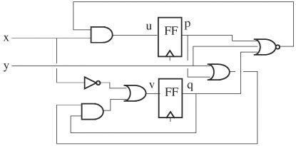
As seen in the previous examples, there are many ways to parameterize a function, and parameterized functions of various complexity result. For a more complete study of parameterization, consult the bibliography.
We started the chapter with decision diagrams. First, the BDD was studied. We showed how to construct a BDD and reduce it to canonical form. The reduction procedure consists of two steps: removing nodes with both edges that point to the same node and merging isomorphic subgraphs. Then we discussed operations on BDDs and how various Boolean manipulations can be cast into ITE operations, and provided algorithms for computing the Boolean operations. Next we examined the effect of variable ordering on BDD size, and introduced static and dynamic variable ordering algorithms.
We then discussed other variant forms of decision diagrams, which include SBDDs, edge-attributed BDDs, ZBDDs, OFDDs, and pseudo Boolean functions. Of the pseudo Boolean functions, we studied ADDs and BMDs.
We next examined how decision diagrams can be used to check the functional equivalence of circuits. In particular, two practical techniques to reduce complexity were mentioned: node mapping and constraining.
As an alternative to decision diagrams, we introduced the Boolean satisfiability problem and presented two methods. The first method, the resolvent method, relies on generating clause resolvents to eliminate variables until the formula or clauses can be easily inferred using the pure literal rule or the unit clause rule. The second method, a search-based method, has the main components of selecting branches, inferring results, and backtracking.
Symbolic simulation, contrary to traditional simulation, is capable of simulating multiple traces simultaneously. We introduced the basic idea of symbolic simulation and common techniques to reduce complexity by constraining variables and parameterizing states.
1 | For the BDD in Figure 8.44, do the following:
|
2 | Reduce the BDD in Figure 8.45. Which rules of reduction did you use? |
3 | Synthesize from BDDs.
|
4 | Perform the following operations on the BDDs in Figure 8.46:
|
5 | Find a good variable ordering for the circuit in Figure 8.47 and build an ROBDD using this variable ordering. |
6 | Apply sifting operations to the BDD constructed in the previous problem. Did you find a better ordering? |
7 | Find an optimal variable ordering for the following function. Can you prove that it is an optimal variable ordering? |
8 | Make the BDDs in Figure 8.48 into an SBDD. What is the ratio of the number of nodes before and after the merge? |
9 | Convert the BDD in Figure 8.44 into a BDD using edge attributes. What is the savings in using an edge-attributed BDD? |
10 | Transform the edge-attributed BDD in Figure 8.49 to the standard form. |
11 | Convert the function in Figure 8.50 to a ZBDD. |
12 | Derive the function of the ZBDD in Figure 8.51, assuming the variables of the functions are a, b, c, and d. |
13 | Five bits are used to encode 32 objects: bits a, b, c, d, and e. For the following, use variable ordering a, b, c, d, and e.
|
14 | Derive a Reed–Muller form for the following function by first constructing an OFDD: |
15 | Reduce the OFDD in Figure 8.52 and derive its function. |
16 | Consider the modulo operator x % y where x and y are integers that can take on any value from 1 to 4. Use an MDD to describe the operation of this modulo function. |
17 | The variables in the following polynomial can have value of either 0 or 1. Represent the polynomial using a decision diagram. |
18 | Derive a BMD for the following function: In the context of a BMD, does every polynomial have a corresponding Boolean function? Why? |
19 | Determine whether the two circuits, F and G, in Figure 8.53 are equivalent.
|
20 | Use the resolvent algorithm to determine whether the following function is satisfiable: |
21 | Use a search-based algorithm to determine satisfiability of the following function. Repeat using a BDD. |
22 | Prove, using symbolic simulation, that for the output f in Figure 8.54, zeros at output f occur in pairs. The initial state is 11.
|
23 | If the inputs to the circuit in Figure 8.55 are of even parity, parameterize the circuit. |
24 | Suppose the next-state vector of a finite-state machine at a cycle is given by
|