The simplest kind of property involves node values at the current cycle and consists of compositions of propositional operators, called Boolean operators, with operands being the node values. This kind of property is combinational in nature. An example property is that, at most, one bus enable bit is high at any time. Most interesting properties are sequential and involve values spanning over a period of time. A propositional property cannot describe variables over time. For example, it cannot express the value of a node from the last clock cycle.

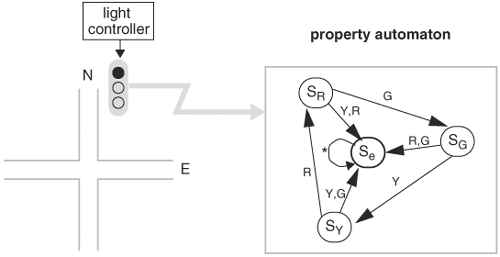
A sequential property can be described using a finite-state automaton, called a property automaton, which monitors the behavior of the circuit by taking as inputs the inputs and states of the circuit. If the property under verification succeeds, then certain designated states in the property automaton are reached. The property automaton can also be constructed to represent failures when certain states are reached if the property fails. Example 9.1 illustrates property specification with an automaton.

Figure 9.1. Property automaton and its interaction with the traffic light controller

Describing temporal behavior using finite-state automata can be cumbersome for many properties and thus error prone. Therefore, a more concise and precise language is needed for specifying temporal properties.

The temporal logic to be introduced in this section is well developed and used widely in verification literature. Although rarely used as a property language in practice, it serves as a means for explaining the underlying theory in model checking. Knowledge of the logic is instrumental in understanding the essential concepts of temporal properties.

Time can be modeled as continuous or discrete. In a discrete model, time is represented by an integer; in a continuous model, by a real number. In this section we are concerned only with discrete time. Furthermore, let’s assume the discrete time points are evenly spaced, and each state transition in an automaton occurs in exactly one time unit. So instead of explicitly stating time, a sequence of state transitions represents the progress of time. Example 9.2 demonstrates the use of state transitions to represent progress of time.

Example 9.2

The finite-state automaton in Figure 9.2A accepts input symbols a, b, or c. Consider a run on input sequence bcabbccaaa... Each time an input symbol is taken, the automaton makes a transition. The sequence of state transitions activated by the input sequence, shown in Figure 9.2B, represents the progress of time. Each state denotes a time instance. In this run, every state has only one successor state. Translating to time instance, we say that every time instance has only one successor time instance.

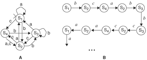
Figure 9.2. This sequence of state transitions represents a progress of time. (A) A state transition diagram (B) Sequence of state transitions on input sequence bcabbccaaa...

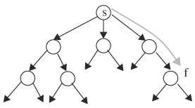
Now, consider the input sequence c{a,b}*{b,c} ..., where the symbols enclosed within {} are possible inputs at that time instance and * denotes any input symbol. Thus, the input symbol at time 1 is c; at time 2, either a or b; at time 3, any input symbol that can be either a or b or c; at time 4, either b or c; and so on. This phenomenon of having multiple possible input symbols is a form of nondeterminism. At time 1, on input c, the transition is from state S₁ to S₄. At time 2, because the input can be either a or b, S₄ can transit to either S₂ on a or S₃ on b. At time 3, because there are two present states, S₂ and S₃, we need to consider them separately. At each of the present states there are three possible inputs. Therefore, there are a total of six next states, although they are not necessarily distinct. At time 4, six present states on two possible inputs produce 12 next states, and so on. This computation of next states represents all computational possibilities of the automaton on the input, and these possibilities are shown in Figure 9.3. Note that every time instance can have more than one successor time instance, and this branching phenomenon is caused by nondeterminism in the input sequence. Other forms of nondeterminism, such as multiple initial states and multiple transitions from a state on the same symbol, also cause branching.

Figure 9.3. A branching state transition tree

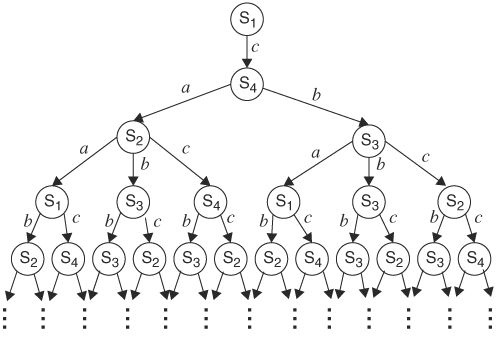
To enumerate all possible computational behavior of a finite-state automaton, we use the input sequence that consists of all possible symbols at each and every time step: *** .... The resulting state traversal is all possible computations by the finite-state automaton and is an infinite tree of state transitions.

Although engineers are more familiar with finite-state machines, an equivalent temporal structure, called a Kripke structure, is widely used in formal verification literature. A Kripke structure is intuitively a state diagram without inputs and outputs, and its transition function depends on the present state only. Associated with each state is a set of variables that are true at the state. More precisely, a Kripke structure K over a set of propositional variables is a 4-tuple K = (S, S₀, T,L), where S is a set of states, S₀ is a set of initial states, T is a total transition relation that maps the present state to a set of next state (a transition relation is total if for every state there exists a next state), and L is a labeling function that associates each state with a set of propositional variables that are true at that state.

An example Kripke structure over propositional (Boolean) variables a, b, and c is shown in Figure 9.4. We use the convention that a variable is true at a state if it is labeled at the state; otherwise, it is false. In the Kripke structure, for example, variables b and c are true and variable a is false at state S₁ because b and c are labeled but not a.

Figure 9.4. An example Kripke structure

Although without inputs, a Kripke structure captures the operations of a finite-state machine by encoding the inputs of the finite-state machine into states in the Kripke structure. Conversely, a Kripke structure can be transformed into a finite-state machine. To transform a finite-state machine into a Kripke structure, each state in the automaton is processed one by one. At a given state, all incoming transitions are partitioned according to their input symbols. Transitions on the same input symbol are grouped together. Then, the state is split into a number of states equal to the number of groups. Each newly formed state then includes the input symbol in its set of labels, and the symbol on the transitions is removed.

If an input has more than one selection (in other words, is nondeterministic, such as {a,b}), all possible values are considered. This can be achieved by transforming the transition with the nondeterministic input into multiple transitions, each taking on one of the possible values. Example 9.3 illustrates this transforming process.

Example 9.3

Transform the finite-state machine in Figure 9.5A into a Kripke structure. The state machine has two binary inputs, a and b. First, because state S₁ has only one deterministic incoming transition—namely, a = 1, b = 0—it does not need to be split. State S₂ has two incoming transitions—namely, a = 0, b = 1 and a = 1, b = 1. Therefore, S₂ splits into two states, each corresponding to an input value, S₂₀ and S₂₁, where S₂₀ is the state when a = 0, b = 1 and S₂₁ is the state when a = 1, b = 1. This state splitting is illustrated in Figure 9.5B. For state S₃, there are four incoming transitions and some inputs are nondeterministic. Therefore, we partition the transitions according to the input values. Because there are three possible input values—a = 0, b = 0; a = 1, b = 1; and a = 0, b = 1—S₃ splits into three states—S₃₀, S₃₁, and S₃₂—as shown in Figure 9.6A. At this stage, all inputs to a state are identical and can be removed from the edges to become a part of the state label. Furthermore, we use 3 bits (r, s, and t) to encode the six states as shown in Table 9.1. The state bits that are true are then labeled on the states with the input bits.

Figure 9.5. Transforming a finite-state machine to a Kripke structure. (A) A state transition diagram. (B) State splitting of S₂ in the process of transforming to a Kripke structure.

For example, at state S₂₀, the input value is āb and the state bits are 001. The bits that are true are b and t. Hence, the Kripke state for S₂₀ has labels b and t. The resulting Kripke structure is shown in Figure 9.6B.

The procedure of transforming a finite-state machine to a Kripke structure is summarized here. Conversely, a Kripke structure is a finite-state machine with ε transitions. An ε transition is activated without an input symbol and is a form of nondeterminism.

Continuously unrolling a Kripke structure traces out all paths from the initial states. If the Kripke structure has loops, paths will be infinite and will never reconverge, producing a tree. This tree is called computation tree. Unrolling the Kripke structure in Figure 9.4 produces the computation tree in Figure 9.7. The initial state is the state labeled bc. From the initial state, there are three next states, labeled a, ab, and ac. From each of the next states, come more states. The process continues indefinitely. Note that states that are encountered along different paths are not merged together. Therefore, the resulting structure is a tree structure. Along a path in a computation tree, crossing a state means the passage of one time unit and the variables labeled at the state at that time evaluate to true. Computation trees are an aid to illustrate concepts and algorithms; they are never used in implementing verification algorithms.

Figure 9.7. A computation tree for a finite-state automaton

The time model can be further classified as linear time and branching time. In a linear time model, a time instance has exactly one successor time instance, an example being that of Figure 9.2B; whereas in a branching time model, a time instance can have more than one successor time instance, as in Figures 9.3 and 9.7. In the following discussion on temporal logic, a path is defined as a path in a computation tree and it consists of a sequence of state transitions. A computation tree in a linear time model has only one path, but a computation tree in a branching time model has many paths.

With the temporal structure defined here, the concept of time is captured in a computation tree. To reason about temporal behavior, we define temporal operators and logic based on computation trees, as presented in the following section.

In this section we will study three types of temporal logic: linear temporal logic (LTL), computation tree logic (CTL), and CTL*. In temporal logic, there are two types of formulas: state and path formulas. A state formula reasons about a state (that is, the validity of a formula at a state). A path formula reasons about a property of a path in a computation tree (that is, whether a formula holds along a path). An example of a state formula is b + c at the present state. An example path formula is as follows: If variable a is 1 at the present state, then b + c will be 1 in the future.

LTL assumes a linear time structure and consists of temporal operators to reason about behavior along the path. An LTL formula is either a state formula that is an atomic formula or a path formula.

The two basic temporal operators in LTL are X (neXt) and U (Until). Let the underlying path in the linear time model be π = s₁ → s₂ → ... → s_i → ..., where s_i is a state and the arrows are transitions. Suppose s₁ is the present state and f and g are state formulas. Operation Xf on π succeeds if formula f holds at the next state, s₂. Operation fUg succeeds if f holds until g holds. More precisely, there is k ≥ 0 such that f holds at s_j 1 ≤ j < k and g holds at s_k. Suppose f and g are path formulas. Let us define π_i as the subpath starting at state s_i. Xf on π succeeds if formula f holds at π₂. fUg succeeds if f holds until g holds. More precisely, there is k ≥ 0 such that f holds at π_j 1 ≤ j < k and g holds at π_k.

LTL formulas are constructed using Boolean operators and temporal operators X and U, following these rules:

Rule 2 says that a formula built by applying Boolean operators to existing LTL formulas is also an LTL formula. Rule 3 states the use of the X and U operators. Although X and U are the minimum LTL operators to build LTL formulas, for convenience other operators are used, despite the fact they can be expressed in terms of X and U. Some such operators are

The meaning, or semantics, of LTL operators is shown in Figure 9.8. The formula above a state denotes the validity of the formula at the state. For instance, in Xf, f is false at s₁ but becomes true at s₂. This temporal behavior of f makes Xf succeed. The trace shown for (f R g) is one of several situations in which (f R g) succeed.

Figure 9.8. Semantics of LTL operators

With a branching time model, in which there are multiple paths, CTL* is applicable. CTL* uses the same temporal operators as LTL, but it adds two path quantifiers to cope with multiple paths: A (for all paths) and E (for some path). Quantifiers A and E mirror the universal and existential quantifiers, ∀x and ∃x, in first-order logic, and apply over paths instead of variables. The two path quantifiers are prefixed to formulas, state or path, to create CTL* formulas. The rules for constructing CTL* formulas are divided into two parts: one for state formulas and the other for path formulas.

For state formulas

For path formulas

Note that path quantifier A(f) is not essential and can be expressed as ~E(~f); that is, “f is true for all paths” is equivalent to “there is no path such that f is false.” Therefore, only three operators are basic in CTL*: X, U, and E. Rule 3 of the state formula says that Ef is a state formula and it has the interpretation that if Ef holds at a state, then there is a path starting from the state such that f holds along the path. Similarly, Af holds at a state if all paths starting from the state satisfy f.

Example 9.4

Examples of CTL* formulas are A(fUg), E(FGg), and AG(EF f). If state s has formula A(fUg), then the formula succeeds if for all paths starting at state s, fUg succeeds. E(FG g) succeeds at state s if there is a path starting at s such that it eventually reaches a state r, at which Gg succeeds. AG(EF f) states that at all nodes along all paths starting at state s (EF f) succeed.

Consider the computation tree shown in Figure 9.9. A formula next to a node means that the formula succeeds at the node. Assume that formula f succeeds at all descendent nodes of nodes 1, 2, 5, and 6; and formula g succeeds at all descendent nodes of nodes 3 and 4. Thus, A(fUg) succeeds at node s because all paths starting at s satisfy f along the paths until g succeeds. E(FG g) succeeds at nodes s, v, and r, because there is a path—the path that ends at node u—that leads to the subtree where g succeeds globally. However, E(FG g) fails at node t, because all paths from node t eventually lead to nodes where only f holds. Formula AG(EF f) succeeds at node t, because all path nodes eventually lead to success of f, but fail at node v, because the paths passing through node u have nodes that never see f succeed—namely, all the nodes below, including node u.

Figure 9.9. Examples of successful CTL* formulas

CTL derives from CTL* by allowing only certain combinations of path quantifiers and temporal operators, and hence is less expressive but easier to verify. The syntax of CTL is defined as follows.

State formulas:

Path formulas:

Comparing these rules with those of CTL*, we notice that in CTL if f is a path formula, then the only way to expand the formula is through path quantifiers E and A (rule 3). Furthermore, the only way to obtain a path formula is through temporal operators X and U.

If we include derived temporal operators F and G, then CTL has only eight base operators—namely, AX, EX, AG, EG, AF, EF, AU, and EU. Furthermore, five of these base operators can be expressed in terms of EX, EG, and EU. That is,

AXf = ~EX(~f)

AF(f) = ~EG(~f)

AG(f) = ~EF(~f)

EF(f) = E( TRUE U f)

A(fUg) = (~E(~gU(~f)(~g)))(~EG(~g))

The semantics of these eight base operators and computation trees that succeed them are enumerated in Table 9.2.

Thus far we do not distinguish paths to which temporal formulas apply, but there are situations when we are only interested in verifying formulas along certain paths. One common such path constraint is a fairness constraint. The term fairness originates from protocol verification, in which a protocol is fair if a persistent request is eventually granted so that an infinite number of requests would warrant an infinite number of grants. Now the usage scope of “fairness” has been extended beyond protocol verification, and it is often associated with situations in which some states or transitions are visited infinitely often. As an example of checking a formula only along fair paths, consider verifying that a bus arbitration protocol handles prioritized requests correctly. Because this priority property is built on top of a fair bus arbitration protocol—fair in the sense that every request will be eventually granted—we should assume that the protocol is fair and will be interested in checking the priority property along fair paths only.

A fairness constraint may be expressed in several ways. In a Buchi automaton, a fairness constraint F is defined as a subset of states. Thus, a path is fair if the path visits some state in F infinitely often. At first it may be puzzling to see the term infinitely often used in a finite-state automaton. The term infinitely often makes more sense if we recall that a path in a computation tree is always an infinite path, even though the set of states is finite. The infinite paths are a result of unrolling loops an infinite number of times. Furthermore, an infinite path must visit some states infinitely often. If we denote the set of states visited infinitely often along path π by inf(π), then π is fair if inf(π) ∩ F ≠ Ø. Another way of expressing fairness is the definition used in a Muller automaton in which a fairness constraint F is a set of edge subsets. A path is fair if the edges traversed infinitely often by the path are an edge subset of F.

Furthermore, a fairness constraint can be in the form of a CTL formula. In this case, a fair path makes the formula true infinitely often along the path. Let φ be a CTL* formula for a fairness constraint and f be a CTL* formula to be verified for all fair paths with respect to φ. The expression for φ to be true infinitely often is GF(φ), which means that, along a fair path, φ will eventually hold at all nodes along the path. Thus, φ holds infinitely often. A weaker form of this concept of “infinitely often” is FG(φ), which means “almost always.” Given this interpretation, the statement that f succeeds with respect to fairness constraint φ is A(GFφ → f), which says that along all paths for which GF(φ) succeeds (in other words, all fair paths), f also succeeds. Similarly, a weaker form is A(FGφ → f).

Note that the previous fairness expressions are not CTL formulas. Thus, fairness constraints can be expressed in CTL* but cannot be directly expressed in CTL. Thus, when checking CTL formulas with fairness constraints, the checking algorithms must ensure that only fair paths are examined. We will look at checking CTL formulas with fairness constraints later.

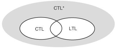
Expressiveness of logic is the scope of properties the logic can express. Before we can compare, we should address the differences in temporal models underlying CTL*/CTL and LTL. The former assumes a branch time model whereas the latter assumes a linear time model. To have a common ground, we interpret an LTL formula f as Af when it is used in a branching time model. An LTL formula must hold for all paths in a branching time model.

Clearly, CTL and LTL are proper subsets of CTL*, because CTL follows a restricted set of formula construction rules and LTL cannot have path quantifier E. Hence, the real question is the relative expressiveness between CTL and LTL. Because in a CTL formula every temporal operator must be preceded by a path formula, it can be shown that the LTL formula A(FGg) cannot be expressed as a CTL formula, but it is an LTL formula. Conversely, because an LTL formula can only have path quantifier A, it can be proved that there is no LTL equivalent formula for CTL formula AG(EFg). Obviously, there are formulas that are both LTL and CTL formulas. Finally, by ORing formulas A(FGg) and AG(EFg), A(FGg) + AG(EFg), we have a CTL* formula that is expressible in neither LTL nor CTL. Therefore, we conclude that (1) CTL and LTL are strictly less expressive than CTL* and (2) neither LTL nor CTL subsumes the other. Figure 9.10 is a visualization of this conclusion.

Figure 9.10. Relative expressiveness of CTL*, CTL, and LTL

SystemVerilog extends the Verilog language into the temporal domain by including sequences and operators for sequences. A sequence specifies the temporal behavior of signals. The key constructor of sequence is the cycle delay operator ##. Operand of ## can be a single integer or a range of integers. For instance, sequence x ##3 y means that y follows x after three cycles, and sequence x ##[1,3] y means that y follows x after a number of cycles ranging from one to three. For instance, the next operator X in CTL* is simply ##1 and the future operator F is ##[1,$], where $ stands for infinity. Sequence operators create complex sequences from simple ones. Example sequence operators are AND, OR, intersect, implication, throughout, and within. For more details on SystemVerilog temporal language, refer back to Section 5.5, SystemVerilog Assertion.

Let us assume that a property automaton has certain states marked as error states that indicate, when reached, the design has an error. The property automaton accepts as input the design’s output and state, and transits accordingly. To verify that an error state can or can never be reached, we need to form a product machine by composing the design machine with the property machine. A state in this product machine consists of two components: one from the design machine and the other from the property machine. Therefore, a state of the product machine is an error state if it contains an error state from the property machine. So, the design has an error if and only if an error state in the product machine is reachable from an initial state. Therefore, the problem of verifying whether a design has an error becomes the problem of deciding whether the set of reachable states of the product machine contains an error state. This procedure is summarized here:

Example 9.7

In a game of two players, each player tosses a die and compares the face values. If player A has a higher value, player A’s score increases by 1, unless it is 2, in which case it becomes 0. Furthermore, B’s score is decreased by 1, unless it is 0, in which case it remains the same. On the other hand, if player B has a higher value, these scoring rules apply except the roles of A and B are reversed. If both dice values are equal, their scores stay unchanged. The properties to verify are

1. Is it possible for both players to tie at the score of 1?

2. How about for both to tie at 2 apiece?

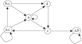
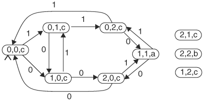
First, we need to construct two automata describing the scores of players A and B. The input to the automata is either 0 or 1. Input 0 means player A has won the toss. Input 1 means player B has won the toss. The states represent the score of the player. Based on the rules, the automata are as shown in Figure 9.11A. Next we construct an automaton to describe both properties. The automaton has three states: State a is that both players’ scores are equal to 1; state b, both players’ scores are equal to 2; and state c, all other cases. The property automaton takes as its input the player automata’s present states.

Figure 9.11. (A, B) Automata for players’ score (A) and property automata (B)

To determine the properties we need to compose the three automata and check reachability. The composite automaton is shown in Figure 9.12. A state in the composite automaton consists of three components, one from each of the three automata. Therefore, property a is affirmed if and only if there is a composite state that contains component a. Similarly, property b is verified if a composite state containing component b is reachable. Because state (1,1,a) is reachable from initial state (0,0,c), property a is true. Indeed, input sequence 1,1,0 will make both players’ scores equal to 1, and there are infinitely many such sequences. On the other hand, no state with component b is reachable; thus, property b is false. It is impossible for both players’ scores to be tied at 2.

Figure 9.12. Composite automaton for checking properties

The design process can be viewed conceptually as a transformation from specifications to final implementation by gradually refining each part of the specification until all parts have been implemented. Refinement turns a more abstract form of design specification into a more specific form. A more abstract version of a design has more nondeterminism, whereas a more specific version contains more concrete details, and hence less freedom. For instance, a 32-bit adder specification is just x = a + b, where a and b are 32-bit variables and x is a 33-bit variable. This specification leaves it open as to how it should be implemented, be it a carry bypass or a ripple adder. This “unspecified” part is freedom, or nondeterminism, in specification. An example of refinement is turning a 32-bit adder specification into a concatenation of two 16-bit adders. Even though the 16-bit version still has freedom for further refinement, it is less abstract than the 32-bit version of the specification. Therefore, as an initial set of specifications goes through stages of refinement, the design becomes more and more specific, and eventually all nondeterminism is removed and a final implementation takes form. At each stage of the transformation, it is necessary that a refined version preserve all the properties in a more abstract version. Using the adder example, the adder at each refinement stage must add correctly. This method of verifying properties preserved at each refinement stage is called refinement verification, and it can be done using language containment.

A design is characterized by the sequences of state transitions it can produce. Because a design can be regarded as a forever-running automaton, all sequences of state transitions in the design are infinite. An automaton accepting infinite input sequences or producing infinite state transition sequences is called an ω automaton. Because the sequences are infinite, the usual acceptance condition that a final state is reachable has to be expanded to cope with sequences of infinite length. One such enhancement is to designate some states or edges as acceptance states or edges. An input string is accepted if the input drives the automaton to visit an acceptance state or edge infinitely often.

Example 9.8

The ω automaton in Figure 9.13 accepts infinite sequences, and edge E is an acceptance condition so that those input sequences traversing edge E infinitely often are accepted. Input sequence 0 101 101 101 101 101 ... traverses E infinitely often and thus is accepted, but neither sequence 0011111111 ... nor 0 1000 1000 1000 ... is accepted.

Figure 9.13. A ω automaton and its acceptance condition

In the following discussion we will refer to an ω automaton simply as an automaton. The set of all accepted sequences is the language of the automaton. Furthermore, we will refer to a more abstract version of a design as the property, and a less abstract version as the design. This is consistent with the fact that a property, being part of a specification, is usually more abstract than the design.

Therefore, a refined design (design) preserves the specifications of a more abstract design (property) if every string accepted by the design is also accepted by the property. If not, there is a design behavior that deviates from the property behavior, and the design fails the property. In other words, a property is satisfied if the language of the design is contained in the language of the property. Let L(D) and L(P) be the languages of the design and property respectively. To check language containment L(D) ⊆ L(P), we need to make use of the fact that L(D) ⊆ L(P) if and only if is equivalent to the language of the complemented automaton, L(), if it exists. For Buchi automata, complemented Buchi automata are also Buchi automata. is equivalent to the language of product machine . Consequently, L(D) ⊆ L(P) if and only if . Therefore, checking language containment reduces to checking language emptiness of the product automaton. This identity is visualized in Vann diagrams, as shown in Figure 9.14.

Figure 9.14. Equivalence between containment and empty intersection

A machine has empty language if no string is accepted by the machine—namely, no acceptance state or edge is traversed infinitely often. To test whether a state or an edge is traversed infinitely often, we need to determine whether there is a loop in the state diagram that contains the acceptance state or edge, and to determine whether the loop is reachable from an initial state. If such a loop exists, a run that starts from the initial state, enters the loop, and traverses the loop infinitely often produces an acceptable infinite sequence. Hence, the language is not empty. On the other hand, if no such loops exist, the language is empty. Therefore, language containment becomes a reachability problem. This verification algorithm using language containment is as follows:

When verifying properties expressed in CTL formulas, we assume a Kripke structure for the design and present the algorithms based on the structure. Hence, verifying a CTL formula means determining all nodes in the Kripke structure at which the CTL formula holds, and if there are initial states, all initial states should be among those nodes. Therefore, checking a CTL formula is done in two steps. The first step finds all nodes at which the formula holds and the second step determines whether all initial states are contained in the set of nodes. Because the second step is trivial in comparison, we will only discuss the first step in this section. Verifying a CTL formula is done by induction on the level of the formula—in other words, by verifying its subformulas level by level, starting from the variables and ending when the formula itself is encountered.

Recall that labeled at each node of a Kripke structure are variables that are true, and the missing variables are false. Let’s extend this labeling rule to include formulas or subformulas that evaluate true at the node. To begin, the subformulas at the bottom level of a CTL formula (made of variables only) are simply the labeled variables at the nodes. At the next level we need to consider two separate cases. In the first case, the operators are Boolean connectives, such as AND and NOT. In this case we will only consider AND and NOT operators because all other Boolean operators can be expressed in these two. At a node, if both operand formulas are true at the node, the resulting AND formula is true at the node and it is labeled at the node. If the operand formula is not true (in other words, it is missing at a node), then the resulting NOT formula is true and it is labeled at the node. In the second case, the operators are CTL temporal operators. We only need to consider EXf, E(fUg), and EG(f), because all other CTL operators can be expressed in these three.

To verify EXf, we must assume formula f has been verified. In other words, all nodes at which f holds are labeled with f. Then, every node with a successor node that is labeled with f is a node satisfying EXf. Therefore, all these nodes are labeled with EXf. This is summarized as follows:

To verify E(fUg), we need to assume formulas f and g have been verified. Then, E(fUg) is true at a node if there is a path from the node to a g-labeled node, and at every node along that partial path f is labeled but g is not. This process can be described by induction on its successors as the following: A node satisfies E(fUg) if g is labeled at the node or f but not g is labeled at the node and its successor is either labeled g or E(fUg). This is summarized as follows:

Finally, to verify EG(f), we again need to assume f has been processed. The semantics of EG(f)—there is a path along which f is true at every node—together with the fact that the path is infinite in a finite Kripke structure implies that EG(f) is true at a node if there is a path from the node to a loop of states such that f is true along the path from the start to an entry to the loop and f is true at all the nodes in the loop. This understanding gives rise to the following algorithm. First we remove all nodes from the Kripke structure that do not have label f. Therefore, every node remaining has label f. Second, we determine all SCCs in the resulting structure. Finally, EG(f) is true at a node if there is a path from the node to an SCC. This algorithm is as follows:

To check other CTL temporal operators, one can either express the operator in terms of the three base operators and apply the previous algorithms or check the operator directly on the Kripke structure.

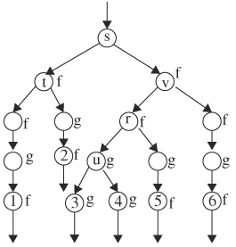
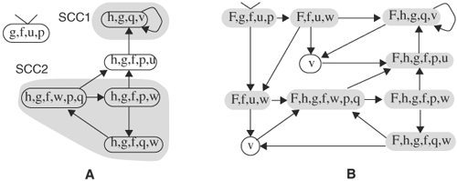
Example 9.9

We can verify the CTL formula on the Kripke structure shown in Figure 9.15A. There are five variables: u, v, p, q, and w. This formula can be broken into three levels. The first-level formulas are propositional: and g = p + q. The second-level formula is h = EGg. The third-level formula is F = E(fUh).

Figure 9.15. Verifying CTL formula E(U(EG(p + q))). (A) Original Kripke structure. (B) Kripke structure after f and g are verified.

We first label the nodes at which the first-level formulas are true. Formula is true at a node if the node does not have label v. Formula g = p + q is true at a node if the node has either label p or q. The result is shown in Figure 9.15B. To check formula h = EGg, we remove nodes without label g and find all SCCs in the resulting graph, as shown in Figure 9.16A. Then all nodes that can reach an SCC are labeled with h. We annotate these h labels to the Kripke structure, as shown in Figure 9.16. Finally, in checking formula F = E(fUh), we label a node with F if either it is labeled h or it has label f, but not h, and it has a successor labeled h or F. The states in which the formula holds are shaded in Figure 9.16B. Because the initial state is among these states, formula holds for the machine represented by this Kripke structure.

Figure 9.16. Checking EG(g) and E(fUh). (A) Kripke structure after EG(g) verified. (B) Final Kripke structure after E(fUh) is verified.

If you are interested in checking CTL* and LTL formulas, please consult the bibliography. CTL model checking can also be done using the so-called fix-point operator and we study this method in a later section.

Checking with fairness constraints means that only the paths satisfying the fairness constraints are considered. Such paths are called fair paths. A fairness constraint can be sets of states or CTL formulas, which we call fair state sets and fair formulas respectively. A fair path traverses each of the fair state sets infinitely often, or each of the fair formulas hold infinitely often along the path.

In the following discussion, let’s assume fairness constraints are expressed as a set of states. The result can be extended to sets of states or a set of fair formulas. As we discussed in a previous section, CTL formulas with fairness constraints cannot be expressed as CTL formulas. Thus, we have to enhance our CTL checking algorithms to deal with fairness constraints.

Because we are dealing with an infinite path in a finite structure, a fair path is a path that emanates from a state and reaches an SCC that contains the fair states or satisfies fair formulas. Therefore, a fair path starting from a node can be identified in three steps:

If step 3 succeeds, then there is a fair path starting from the state. These three steps form an algorithm for determining all states that have a fair path. If we define a fairness variable fair such that it is true at a state if there is a fair path starting from the state, then this algorithm verifies formula fair (in other words, it labels all states in which fair is true).

Because all CTL operators can be expressed in terms of the three operators EX(f), E(fUg), and EG(f), we just consider checking these three with fairness constraints. As usual, we need to assume f and g have been processed according to fair semantics.

For EX(f) to be true at a state, there must be a fair path starting at the state and f holds at the next state. We then make use of the fairness variable fair. Note that if fair holds at state s, then fair also holds at all states that can reach s. Then, EX(f) is true with fairness constraints if and only if f holds at the next state and there is a fair path starting from the next state. In other words, EX(f) holds with fairness constraints if and only if EX(f · fair) holds in the ordinary CTL semantics without fairness. That is, we can use an ordinary CTL checker to verify EX(f · fair) with a passing that means EX(f) holds with fairness constraints.

Formula E(fUg) with fairness constraints means that there is a fair path along which fUg holds. If a such fair path exists and fUg holds along the path, then g · fair also holds. Therefore, E(fUg) holds with fairness constraints if and only if E(fU(g · fair)) holds in the ordinary CTL semantics without fairness constraints.

The procedure to check EG(f) at state s with fairness constraints is as follows: First, all states without label f are removed. Second, all SCCs are determined. Third, all SCCs that do not contain the fair states are removed. Finally, we need to determine whether state s reaches one of the remaining SCCs. If the last step succeeds, it implies that state s reaches an SCC that contains all fair states. Then, the path starting at s, reaching this SCC, and traversing the fair states infinitely often is a fair path along which f holds globally. Therefore, EG(f) holds at s subject to the fairness constraints.

Recall that a finite-state machine is a quintuple, (Q, Σ, δ, q₀, F), where Q is the set of states, Σ is the set of input symbols, δ is the transition function with δ : Q × Σ → Q, q₀ is an initial state, and F is a set of states designated as acceptance or final states. The transition function δ is based on the current state and an input symbol, and it produces the next state. Another way to represent δ is with q^{i + 1} = δ(qⁱ, a), where qⁱ is the present state at cycle i, q^{i + 1} is the next state, and a ∊ Σ is an input symbol. The key to model and traverse a finite-state machine symbolically lies in representing a set of states as well as the transition function as characteristic functions.

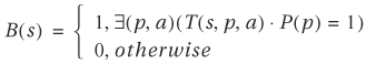
A characteristic function Q(r) for a set of states S is such that

If each state is encoded in bits, then the characteristic function is just a disjunction of the terms representing all the states in the set. For instance, if eight states are encoded with 3 bits—a, b, and c—the characteristic function Q(a, b, c) representing the set consisting of state 101 and 110 is , which is 1 if and only if abc = 101 or 110.

To represent the state transition function we would define the characteristic function as follows:

where p is a present state, n is a next state, and a is an input symbol. That is, T(p, n, a) is 1 if and only if the present state, next state, and the input symbol satisfy the transition function. This method of representation using characteristic functions is called relational representation. Thus, T(p, n, a) is sometimes called a transition relation. Another method of representation is functional representation: The transition function is represented as q^{i + 1} = δ(qⁱ, a). An important benefit gained through the use of characteristic functions is that all the arguments (p, n, and a) can be a set of states and a set of input symbols, as opposed to a single state. In contrast, a transition function representation cannot represent the situation in which more than one next state exists for a given present state and an input symbol.

To demonstrate symbolic traversal, we need to compute the set of all possible next states, N(s), from a given set of present states, P(s), under all input symbols. N(s) is a characteristic function for the set of next states; thus, s is a next state if there is a present state p and an input symbol such that T(p, s, a) = 1. Because p is a present state, P(s) = 1. The statement “there is a” translates into the existential quantifier. Putting these together symbolically, we have

Example 9.10

Consider the circuit in Figure 9.17 and compute the following:

Figure 9.17. A circuit for symbolic traversal

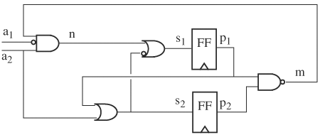
1. Derive a relational representation for the transition function.

2. Compute the next state if the present state is 00 and the input symbol is 10.

3. Compute the set of all next states if the present state is either 00 or 11.

Based on the circuit diagram we can relate the next-state bits s₁ and s₂ to present-state bits p₁ and p₂, and input bits a₁ and a₂, as

s₂ = p₁ + a₂

To make these equations into a characteristic function, or a relation, we form a function that becomes 1 if and only if the right-hand side of the previous equation is equal to the left-hand side. Therefore, the transition relation is

The next state, given the present state 00 and input 10, is T(0,0,s₁,s₂,0,1), which simplifies to s₁ · s₂. Thus, the next state s₂s₁ is 11, consistent with a calculation from the circuit diagram.

For step 3 we first must represent the set of present states, 00 and 11, with a characteristic function: . The set of all next states for all possible inputs is

Recall that ∃(x)f(x) = f_x + f-_x. Thus, the previous expression becomes

After simplification, it becomes

Because N(s₁,s₂) is a characteristic function for next states, any values of (s₁,s₂) that make N(s₁,s₂) evaluate to 1 are next states. Therefore, the next states (s₁,s₂) are 10, 01, and 11. I leave you to confirm that the set of next states is correct. To appreciate the elegance of relational representation, it is an interesting exercise to repeat these computations using functional representation.

The transition function of a finite-state machine takes in a set of present states P(s) and produces a set of next states N(s). N(s) is called the image of P(s) under the transition function. Conversely, P(s) is called the preimage of N(s). Starting from a set of initial states I(s), we can iteratively compute the image of the initial states, then the image of the image just computed, and so on. When the image contains all reachable states, further computations will not yield a larger image. At this stage, the image is identical to the preimage. When this occurs, the computation stops. Image computation is also called forward traversal, because each iteration of computing next states is one cycle advance in time. The algorithm computing reachable states from a set of initial states is as follows:

Every step in the previous image computation algorithm is executed as BDD operations, as opposed to graphical operations. First, the transition relation and state set S are represented using BDDs. In step 2, the BDD of S(p) is ANDed with that of T(p, s, a), and the result is existentially quantified, again as a BDD operation. In step 3, checking whether S = R is executed by comparing the BDDs of S and R. The result is a BDD for the characteristic function of all reachable states.

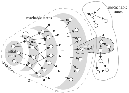
To verify that a design satisfies a safety property (such as, an error should never occur), the property is expressed as a set of faulty states such that the property is violated if any of these faulty states is reached. This set of faulty states is represented by a characteristic function in the form of a BDD: F(s). This property is satisfied if and only if none of the bad states is contained in the set of reachable states, R(s). Symbolically, R(s)·F(s) = 0. The AND of these two BDDs is identically equal to constant 0. At any iteration of computing R(s), if (R(s) ·F(s)) ≠ 0, then an error state is reachable and the property fails so that no further computation is necessary. Furthermore, if R(s) ·F(s) = D(s) ≠ 0, then BDD D(s) is the set of all reachable faulty states. This method of verification using forward traversal is visualized in Figure 9.18. The crescents represent the states reached at each iteration—N(s). In the diagram, state e, a faulty state, is reachable from an initial state at iteration n, implying the design contains an error. This verification algorithm is summarized as follows:

Figure 9.18. Verifying safety property using forward traversal

An alternative to using forward traversal is to traverse backward starting from a set of faulty states F(s). Let B(s) be the set of previous states of present state set P(s). Then B(s) is formulated as

Compare B(s) with N(s) and note that the positions of the arguments in the transition function are reversed. Backward traversal is exactly the same as forward traversal if N(s) is replaced by B(s), and I(s) by F(s). At any iteration, if BR(s), the backward reachable set, has a nonempty intersection with the initial state set, then it means that a faulty state is reachable from an initial state and, the design has an error. Backward traversal terminates when all backward reachable states have been reached. Namely, BR(s) remains unchanged during an iteration. For completeness, a backward traversal algorithm and a backward faulty state reachability analysis algorithm are summarized as follows:

Whether forward or backward traversal first reaches a conclusion depends on the design under verification and is difficult to predict in advance. However, one can combine both forward and backward traversal, called the hybrid traversal method. An error is detected whenever R(s) and F(s) or BR(s) and I(s) have a nonempty intersection. The hybrid traversal terminates when either R(s) or BR(s) becomes unchanged.

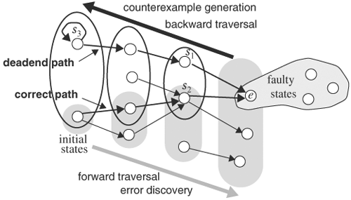
When a verification algorithm declares that an error has been discovered, it should generate an input sequence and an initial state, called a counterexample, so that the designer can simulate the input sequence from the initial state to reproduce the error and debug it. Let’s assume a forward traversal algorithm was used to detect an error, and N_i is N at iteration i. Suppose that a bad state is contained in the ith iteration of the traversal. Then, N_i · F ≠ 0. We then pick a state e ∊ N_i · F as an error state E and, with a slight modification, apply the backward traversal algorithm to the initial state. As we back trace, we want to limit the preimage of backward traversal to be within the image of the forward traversal that found the error to guarantee that we will reach an initial state. Specifically, in the first iteration of backward traversal, S = {e}, we compute BN₁, the preimage of S. Before computing the preimage of BN₁ in iteration 2, instead of setting S = BN₁, we intersect BN₁ with the image at iteration i -1 of the forward traversal, N_{i - 1}. In other words, we set S = BN₁ · N_{i - 1}. The reason for performing this intersection is to ensure that we back trace from states that also lie in the forward-traversed image so that an initial state will be reached. Without this intersection, it is possible that we would never reach an initial state from the faulty state, as explained next. We then compute the preimage of S. The traversal stops when an initial state is contained in BN. Because it took i iterations for the forward traversal to reach a faulty state, it must take at most i iterations to reach an initial state from the faulty state. However, an initial state may be reached in fewer than i iterations.

This algorithm of generating a counterexample is depicted in Figure 9.19. In the figure, the shaded ovals are forward reachable states, whereas the unfilled ovals are backward reachable states. In three iterations, a faulty state, e, is reachable from the initial state. To generate a counterexample from this faulty state, we can back trace from e. In the first backward traversal, two states lie in the preimage of e, s₁, and s₂. s₁ does not lie in the forward traversal image, but s₂ does. We should pick s₂ in our next back-tracing iteration to ensure that we will eventually reach an initial state. If we pick s₁, we would end up in the deadend state s₃ and never reach an initial state, as the upper boldface path indicates. To guarantee that backward-traversed states lie in the forward image, such as s₂, it is necessary to intersect the backward preimage with the forward image, which in this case yields s₂. From s₂, we continue back tracing until it reaches the initial state, as indicated in the lower path.

Figure 9.19. Generating a counterexample for an error found in a forward traversal

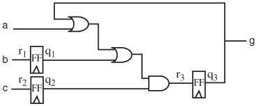
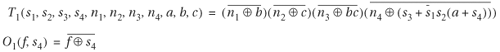
To determine whether two sequential circuits are functionally equivalent, we can just compare their next-state functions using BDDs if their states are in one-to-one correspondence. This was discussed in Section 8.3. However, when two circuits’ states are not in one-to-one correspondence, model-checking technique must be used. The two circuits’ outputs are pairwise XORed, and the XOR outputs are ORed together as output D, as shown in Figure 9.20. Therefore, the two circuits are equivalent if and only if output D is identically 0.

Figure 9.20. Auxiliary circuit for determining sequential equivalence

Let transition functions and output functions of the two circuits be , , , and , respectively, where y, z, s₁, s₂, n₁, n₂, and x are output, present state, next state, and input vectors. The output functions are characteristic functions, that evaluate to 1 if and only if output y or z is the output value at state s and input x. Then, the transition function for the product machine of these two circuits is

Output D is

where is the characteristic function that evaluates to 1 whenever is not equal to . For a single variable, becomes . For vectors, becomes . Suppose I₁ and I₂ are initial states of the two circuits. Then the initial state of the product machine is I = I₁ · I₂. We can apply the faulty state reachability analysis algorithm to this product machine with faulty state function . The algorithm evaluates at each reachable state. If is 1 at a reachable state, the outputs of the two circuits are not equal; therefore, the two circuits are equivalent if and only if the answer from the algorithm is NO.

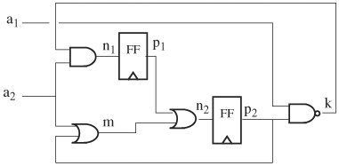
Example 9.11

We can apply the previous algorithm to determine whether the circuits in Figure 9.21 are equivalent, assuming the initial states for both circuits are all zeros. Because the two circuits have different numbers of FFs, there is no one-to-one correspondence between the FFs. Thus, we cannot determine their equivalence by simply comparing their next-state functions. Let’s call the circuit in Figure 9.21A circuit 1 and the other circuit 2.

Figure 9.21. (A, B) Example circuits for determining sequential equivalence

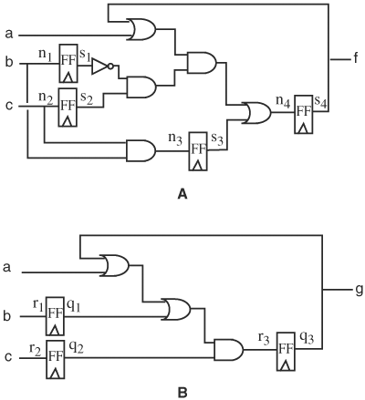
The transition function and output function for circuit 1 are

Similarly, the transition function and output function for circuit 2 are

Thus, the transition function for the product machine is

The initial state is

We can then apply the forward reachability verification algorithm. The set of reachable states in one iteration is calculated by enumerating over all present states and inputs, and is accomplished by quantifying over the present state variables and input variables:

For iteration 2, we first replace the next-state variables with present state variables—namely, replacing n_i by s_i and r_i by q_i. Therefore, the reachable states after one iteration are

Now, we check whether D(f, g, q₃, s₄) has a nonempty intersection with R₁ by forming

which is identically equal to 0. A program can confirm this by building a BDD. However, we will observe that for the expression to become 1 it is necessary that s₄ = q₃ = 0, which implies f = 0 and g = 0. Thus f ⊕ g = 0, making the expression 0.

For iteration 2, the set of states in two cycles is given by

After some calculations, we obtain

Hence, the set of reachable state after two cycles is, after making the present state variable substitutions,

Here we check whether D(f, g, q₃, s₄) has a nonempty intersection with R₂. In this case,

is identically equal to 0, because ( implies s₄ = q₃, which forces f = g and f ⊕ g = 0. Therefore, D · R₂ = 0.

For iteration 3, the set of states reachable in three cycles is given by

and it produces, again after state variable substitutions

The states reachable after three cycles are

Because R₃ = R₂, we have reached all states and the algorithm stops. Therefore, we can conclude that the two circuits are equivalent.

As discussed earlier, one method of model checking is to prove that the language of the design is contained in that of the property. Language containment can be transformed into the problem of deciding whether an automaton has empty language. If an automaton has empty language, then none of the acceptance states is reachable, which is attainable by applying reachability algorithms.

Because most designs are continuously running and do not have final states on which the designs halt, input strings are infinite. To deal with infinite strings, a different kind of acceptance conditions is required. ω-automata accept infinite strings and have the same components as those accepting only finite strings except for the acceptance structure. In a ω -automaton, the set of states or edges that are traversed infinitely often are checked for acceptance. Different kinds of acceptance structures give rise to different kinds of ω -automata. In a Buchi automaton, the acceptance structure is a set of state A, and an infinite string is accepted if some of the states in A are visited infinitely often as the string is run. Let inf(r) denote the states visited infinitely often when input string r, an infinite string, is run. Then r is accepted if inf(r) ∩ A ≠ Ø. The set of all accepted strings is the language of the ω -automaton. Other types of ω -automata are Muller, Robin, and Street, and L-automaton.

Recall that fairness constraints require certain states to be traversed infinitely often. Therefore, fairness constraints can be cast into a form of acceptance conditions of ω -automata. Thus, algorithms in this section apply equally for fairness constraints. Next we will look at the language containment of Buchi automata. Buchi automata are closed under complementation and intersection—meaning that for every Buchi automaton M, there exists a Buchi automaton that accepts the complement of the language of M and a Buchi automaton that accepts intersection of the languages of two Buchi automata. Therefore, for Buchi automata, the problem of language containment becomes the problem of determining language emptiness. More precisely, if M₁ and M₂ are Buchi automata, then there exist Buchi automata M_p and such that and . Therefore, L(M₁) ⊆ L(M₂) if and only if .

A Buchi automaton has empty language if no infinite string traverses any state in A, which implies that no initial state can reach an SCC that contains a state in A. To be able to reason about this symbolically, we first show how transitive closure is computed symbolically, and then we apply transitive closure to language containment.

Recall that the transitive closure of a state is the set of states reachable from the state. Let C(s, q) be a characteristic function for the transitive closure of state q. In other words, C(s, q) = 1 if state s is reachable from q in any number of transitions. Then C(s, q) is calculated in a number of iterations. In the first iteration, C₁(s, q) = ∃(a)T(q,s,a), which is the set of next states. In the second iteration, we compute the image of C₁(s, q) and add to it C₁(s, q)—namely,

The first term is the reachable state in one step from C₁, and, by adding C₁, C₂ is the set of states reachable in one or two transitions. In the ith iteration,

Because the number of states is finite, there is an integer n such that C_{n + 1}(s, q) = C_n(s, q). This happens when all reachable states from q are included. Then, C(s, q) = C_n(s, q).

Once we have computed the transitive closure of a state, the transitive closure of a set of states Q(s) is C(s, Q) = ∃(p)C(s, p)Q(p). The algorithm for computing transitive closure is summarized as follows:

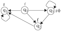
Example 9.12

Compute symbolically the transitive closure of the graph in Figure 9.22. With the states encoding as shown, we can construct the transition relation T(x, y, r, s), where x and y are present state bits, and r and s are next state bits. At state a, the next states are b and c. Thus, the transition relation contains the term . At state b, the next state is b, giving . At state c, the next state is d, and hence the transition term is . Finally, at state d, the next state is b or c, giving . Adding all the terms gives a transition relation of

Figure 9.22. Graph for symbolic computation of transitive closure

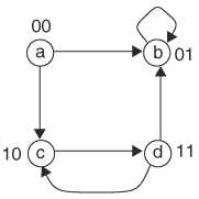
Now we need to follow the previous algorithm to compute the transitive closure of state (xy), C(m, n, x, y).

In step 1,

In step 2,

And

It follows that

Because , and C(m, n, x, y) is not equal to C(m, n, x, y) + N(m, n, x, y), we set

C(m, n, x, y) = C(m, n, x, y) + N(m, n, x, y)

Thus,

Next we must repeat steps 2 and 3 of the transitive closure algorithm:

And

Therefore,

which is equal to C(m, n, x, y). So we are done, and the transitive closure of state (xy) is .

As a check, if xy = 00 (in other words, state a), C(m, n, 0, 0) = m + n, which is 1 for states 10,01, and 11, meaning states b, c, and d are in the transitive closure of state a, as expected. If xy = 01 (in other words, state b), then , meaning only state b is in its transitive closure. Again, this is consistent with what the graph indicates. If xy = 10 (state c), then C(m, n, 1, 0) = m + n, meaning states b, c, and d are in the transitive closure of state c. Finally, If xy = 11 (state d), then C(m, n, 1, 1) = m + n, meaning states b, c, and d are in the transitive closure of state d.

Now we can compute SCCs using transitive closure. Recall that an SCC is a set of states such that every state is reachable from every other state in the SCC. Let SCC(r, s) be the characteristic function of the SCC of state s. Then SCC(r, s) = C(r, s)C(s, r), where C(r, s) is the transitive closure of state s. To understand this equality, refer to Figure 9.23 and consider state p in the SCC of s. We want to show that SCC(p, s) = 1. Because p is reachable from s and vice versa, C(p, s) and C(s, p) are 1. Hence, SCC(p, s) is 1. Conversely, we want to show that SCC(p, s) = 1 implies p is in the same SCC of s. SCC(p, s) = 1 implies that C(p, s) = 1 and C(s, p) = 1, which in turn implies p is reachable from s and vice versa. Therefore, p is in the SCC of s.

Figure 9.23. An SCC illustrating the expression of SCC(r, s)

Now we can apply the previous SCC computing algorithm to check language emptiness. To determine whether a Buchi automaton with acceptance state A(s) and initial state I(s) has empty language, we check whether there is an initial state that reaches an SCC that contains a state in A. First, ∃(r)(SCC(s, r)A(r)) represents all states in an SCC containing an acceptance state. To understand, the formula is 1 if and only if there is a state r that is an acceptance state and it belongs to an SCC. The formula is a characteristic function for all states in the SCC of r. Let C(s) be the transitive closure of initial states I(s). Then, similarly, the state of SCCs reachable from an initial state is given by ∃(q)(SCC(s, q)C(q)). Putting these two conditions together, the state of SCCs reachable from an initial state and containing an acceptance state is

This formula describes an SCC that contains two states, r and v, such that r is reachable from an initial state and v is an acceptance state.

Therefore, a Buchi automaton has empty language if and only if the following expression is identically equal to 0:

Let F(s) be a fairness constraint (a characteristic function of a set of fair states). We can determine SCCs that further satisfy F(s). This is accomplished by further quantifying SCC over F(s):

The algorithm for language containment of Buchi automata is as follows:

Example 9.13

Let us compute all SCCs for the graph in Figure 9.22. The transitive closure is

As a check, the SCC of node d consists of nodes c and d. The SCC of d is given by SCC(m,n, 1, 1) = m, meaning nodes 10 or 11 are in the SCC, as expected. The SCC of node b should be itself. Indeed, , which is satisfied only at node b. The SCC of node c contains c and d. SCC(m, n, 1, 0) = m, giving nodes c and d. Finally, node a does not belong to any SCC. Indeed, SCC(m, n, 0, 0) = 0.

A function y = f(x) has a fix-point if there exists p such that p = f(p), and p is called a fix-point of the function. On one hand, not all functions have fix-points. Function f(x) = x + 1 in a real domain and range does not have a fix-point. On the other hand, some functions have multiple fix-points. For example, f(x) = x² - 2 in a real domain and range has two fix-points: -1 and 2. One way of finding a fix-point is to select an initial value of x, say x₀, and compute iteratively the sequence x₁ = f(x₀), x₂ = f(x₁), ..., x_i + 1 = f(x_i), until x = f(x). This sequence of computations can be regarded as applying mapping f to x₀ multiple times until it reaches a fix-point. The choice of x₀ plays an important role in determining whether a fix-point will be found and which fix-point will be found.

Let’s consider functions with a domain and range that are subsets of states. In other words, functions that take as input a subset of states and produce another subset of states. Let τ(S) denote a such function and τⁱ(S) be i applications of τ to S. In other words, τⁱ(S) = τ(τ(...τ(S))) i times. Furthermore, let’s say that τ(S) is monotonic if A ⊆ B implies τ(A) ⊆ τ(B). Let U be the set of all states. Theorem 9.1 provides conditions on τ so that it has fix-points.

We can call τ^a (Ø) and τ^b (U) the least and greatest fix-point of τ, and denote them by lfp(τ) and gfp(τ) respectively. Now we can express the six CTL operators using fix-point notation. In Theorem 9.2, for brevity a CTL formula stands for the set of states at which the formula holds. That is, formula f stands for the characteristic function λ(s, f) = {s/f holds at state s}. It is for notational brevity that we use this shorthand.

To understand the notation in Theorem 9.2, consider AF(f) = lfp(τ(S)), where τ(S) = f + AX(S). This says that the set of states AF(f) holds is the least fix-point of τ(S). τ(S) takes in a set of states S and computes the set of states with next states that satisfy S. In other words, in S, this result is then ORed with the set of states at which formula f holds. Using characteristic function notation, it is λ(s, AF(f)) = lfp(τ(S)) and τ(S) = λ(s, f) + λ(s, AX(S). Operators AX and EX can be computed without using a fix-point operator, as

and

where T(s, n) is the transition relation of the underlying Kripke structure. The universal and existential quantifiers are computed as conjunction and disjunction as follows:

and

Function τ(S) transforms predicates f and g into a function and is called a predicate transformer.

To have an intuitive understanding of these identities, we need to examine AF(f). AF(f) holds at a state if all paths from the state will eventually lead to states, including the state itself, at which f holds. The least fix-point computation AF(f) = lfp(f + AX(S) consists of a sequence of operations, as shown here.

In iteration 1, τ¹ = f + AX(Ø). The states included in τ¹ are the states at which f holds and the states at which AX(Ø) holds. AX(Ø) contains the states with next states that satisfy Ø, which is not satisfiable. Thus, AX(Ø) gives Ø. Therefore, the states returned by τ¹ are the set of states at which f holds—λ(s, f). Thus, states in τ¹ satisfy AX(f).

In iteration 2, τ² = f + AX(f). The states included are those that satisfy f and all the next states that satisfy f. Thus, τ² satisfies AX(f).

In the ith iteration,

Thus, a state is in τⁱ if it satisfies f or all paths from it reach states that satisfy f in i or fewer transitions. Therefore, states in τⁱ satisfy AX(f). Hence, the states in the least fix-point of τ(S) = f + AX(S) satisfy AX(f). Figure 9.24 shows a Kripke structure and illustrates the progressive inclusion of states through iterations in fix-point computation. The solid circles represent included states, and states labeled f satisfy f.

Figure 9.24. Successive inclusion of states satisfying AF(f) in fix-point computation

Conversely, consider state v that all its paths eventually lead to states satisfying f. Let n be the earliest time when all paths from v have reached states satisfying f. Then v must be included in τⁿ, which is a subset of the least fix-point of τ(S). Therefore, v must be in lfp(τ(S)).

Similarly, AG(f) = gfp(τ(S)), where τ(S) = f · AX(S) expands to

which implies that a state v satisfies AG(f) if it satisfies f, AX(f), AX²(f), and so on, which is equivalent to saying that v satisfies f, and all its next states satisfy f, and all its next next states satisfy f, and so on. This is just what AG(f) is. Other identities can be interpreted similarly.

To complete our treatment of symbolic checking of CTL formulas, we need to examine the case when the formula f is a Boolean formula without CTL operators. We can compute λ(s, f) from the bottom up using the following identities:

and

Note that characteristic functions are represented using BDDs. Therefore, fix-point computation, complementation, and ORing of characteristic functions are executed as efficiently as BDD operations.

Example 9.14

Let’s take a look at in the Kripke structure in Figure 9.25. We use 3 bits—q₂, q₁, and q₀—to encode the eight states. For simplicity, the code of a state is the binary of the state number. For example, s₆ has code 110. The transition relation is

Plugging in the state bits, we obtain

Notice the complexity of the transition function. It is a major source of computational cost. This transition function is used in computing EX(f), as in

To compute , we first compute f = a and , and then E(fUg). The set of the states satisfying atomic formulas, a, consists of s₂, s₃, s₆, and s₇. So, the characteristic function λ(q₀, q₁, q₂, a) is

Similarly, and

From these atomic propositions, we can compute the following:

Now, we have λ(q₀, q₁ q₂, f) = q₁ and λ(q₀, q₁, q₂, g) = . As a check, we label the states with f and g, as in Figure 9.26A. It can be seen that both λ(q₀, q₁, q₂, f) and λ(q₀, q₁, q₂, g) give the correct sets of states.

Next, we use the fix-point formulation to compute E(fUg). That is, E(fUg) = lfp(τ(S)), where τ(S) = g + f · EX(S).

In iteration 1, we have τ¹ (S) = g + f · EX(Ø) = λ(q₀, q₁, q₂, g) = q₂q₁q₀ + . The states included in this iterations are 000, 100, and 111 (or, s₀, s₄, and s₇). They are shaded in Figure 9.26A. This iteration finds the states only satisfy g.

In iteration 2,

where

After simplification, . The states are 000, 011, 100, 110, and 111. They are shaded in Figure 9.26B. This iteration includes states that are labeled g or f, and those with a next state labeled g. The former is a result of iteration 1, and the latter is a result of the current iteration. Because τ²(S) is not equal to τ¹(S), we continue.

In iteration 3,

Substituting the expressions, we get , which is not equal to τ²(S). The states are 000, 010, 111, 100, 110, and 111 (or, s₀, s₂, s₃, s₄, s₆, and s₇). They are shaded in Figure 9.27. The newly added state s₂ is two cycles from a state labeled g.

In iteration 4,

Substituting the expressions, we get , which is equal to τ²(S).

Therefore, we have reached a fix-point. The characteristic function for the states satisfying is . The states are s₀, s₂, s₃, s₄, s₆, and s₇.

Figure 9.25. A Kripke structure for symbolically checking

Figure 9.26. Progressive inclusion of states satisfying . (A) Kripke structure after f and g are verified. (B) Kripke structure after two iteration of τ(s) = g + f · EX(S).

Figure 9.27. States attained in iteration 3 in computing

A fairness constraint φ = {φ₁, ..., φ_n} mandates that all its formulas, φ₁, ..., φ_n, be satisfied infinitely often along a path. A path satisfying φ is called a fair path. Checking a CTL formula f with a fairness constraint φ means that only fair paths are considered and we find all states satisfying f along the fair paths. Because all CTL operators can be expressed in three base operators (EX, EU, and EG), we will study checking of these three operators with fairness constraints. To distinguish CTL checking from CTL checking with fairness constraints, we denote checking with fairness with a subscript φ, as in EX_φ(f), E_φ(fUg), and EG_φ(f). We first compute EG_φ, then EX_φ and EU_φ, which makes use of the algorithm of EG_φ.

EG_φ(f) means that there exists a path along which f holds at every state, and every formula of φ holds infinitely often. In Figure 9.28, EG_φ(f) with φ = {φ₁, φ₂} holds at state

Figure 9.28. A Kripke structure having states satisfying EG_φ(f)

s₁, because path P satisfies f at every state, and it satisfies both φ₁ and φ₂. Similarly, EG_φ(f) holds at s₂, s₃, and s₄. But EG_φ(f) fails at s₀, s₅, and s₆, because path L, the only path, does not satisfy both fairness constraints. EG_φ(f) can be expressed using fix-point notation and ordinary CTL operators

where

When we compare EG_φ(f) with EG(f) = gfp(f · EX(S)), we see that an EU operator is nested inside the EX operator. To get an intuitive understanding of the identity, we must assume there is only one fairness formula—φ = {φ}—and unroll it a couple times.

In iteration 1, τ¹ = f · EX(E(fU(φ))), which holds at state s if f holds at s and its next state satisfies fUφ. Such a state, s₀, is illustrated in Figure 9.29A.

Figure 9.29. Unrolling the fix-point computation of EG_φ(f). (A) A sequence of states after one iteration expansion of EG_φ(f). (B) A sequence of states after two iterations of expanding EG_φ(f).

In iteration 2, τ² = f · EX(E(fU(τ¹ · φ))), which is the same description as τ¹ except for how the path ends—it must end at a state in τ¹, which contains s₀. Concatenating the path described by τ² with the path for s₀ from τ¹, we have the path shown in Figure 9.29B. This path satisfies f at every state and the fairness constraint is satisfied twice. Further iterations simply append paths from the previous iterations. Each iteration only adds states that satisfy f and a state that satisfies φ. At the nth iteration, the resulting path satisfies φ n times. Therefore, the result is a path, or a set of paths, that satisfies f at every state and satisfies φ infinitely often, which is simply EG_φ(f).

To compute EX_φ(f), we use the same technique we introduced in explicit checking of EX_φ(f)—namely, creating variable fair, which evaluates true at a state if there is a fair path emanating from the state. Then EX_φ(f) = EX(f · fair). To obtain the characteristic function for a set of states satisfying fair, λ(s, fair), we use the identity λ(s, fair) = EG_φ(1). Therefore, the set of states satisfying EX_φ(f) is the set of states with next states that are in both λ(s, f) and λ(s, fair). In other words, EX_φ(f) = EX(f) · EG_φ(1). Similarly, E_φ(fUg) = E(fUg · fair), which mandates the ending states also be in λ(s, fair).

Example 9.15

If we take a look at Figure 9.30, we use 2 bits (s₁s₀) to encode the states, and the encoding of a state matches the state’s subscript. With fairness constraint φ = {s₁}, which indicates that states q₂ and q₃ are fair states, we can compute EG_φ(f).

Figure 9.30. Checking fair CTL formula EG_φ(x) with fairness constraint φ = {s₁}

First we calculate the set of states at which f holds. It consists of states q₀, q₁, and q₃, giving . The state set satisfying the fairness constraint is s₁.

In EG_φ(f) = gfp(f · EX(E(fU(S · φ)))), there are two fix-point computations here. The inner fix-point computation comes from E(fU(S · φ)).

In iteration 1 of the outer fix-point computation, τ¹, we need to compute f · EX(E(fUφ)). The inner fix-point computation is E(fUφ) = lfp(φ + fEX(S)). This fix-point computation unfolds as follows:

(a fix-point)

Thus, , giving

In iteration 2 of the outer fix-point computation, we compute . So τ² = f · EX(E(fU(s₁s₀))).

The inner fix-point computation is E(fU(s₁s₀)) = lfp(s₁s₀ + fEX(S)).

So,

a fix-point for the outer fix-point computation. Therefore, the entire computation terminates, giving

Based on this result, only states q₀ and q₃ satisfy EG_φ(f). Examining Figure 9.30, we can confirm that these two states traverse the self-loop at state q₃ satisfy φ infinitely often and every state along the path also satisfies f. State q₁ is excluded because it does not satisfy φ. State q₂ is omitted because it does not satisfy f.

In N(n) = ∃(p, a)(T(p, n, a) · P(p)), a straightforward approach is to compute the conjunction of T(p, n, a) and P(p) first, and then quantify the result over present state p and input a. The result from the conjunction before quantification can be so massively complex that it exceeds allotted memory capacity. Because quantification eliminates variables, the sooner a function is quantified, the smaller the function becomes, and the more efficient the rest of computation involving the function gets. One may observe that P(p) does not involve input variable a and hence it can be taken out from the quantification of variable a. That is, N(n) = ∃(p, a)(T(p, n, a) · P(p)) becomes N(n) = ∃p(∃aT(p, n, a)) · P(p)). This is a consequence of the following identity:

This early quantification of input a on T(p, n, a) is performed once before image computation begins and its result is reused thereafter for all image computations. Therefore, with early quantification, image computation takes two steps: (1) compute τ(p, n) = ∃aT(p, n, a)) and (2) N(n) = ∃p(τ(p, n) · P(p)). Because τ(p, n) has fewer variables than T(p, n, a), the BDD size of τ(p, n) is smaller than that of T(p, n, a). τ(p, n) is the characteristic function for the set of all legal transitions from present state p to next state n.

Example 9.16

We can compare the sizes of the following transition relation with and without early quantification, T(p, q, r, s, a, b) = , where a and b are inputs.

Without early quantification, it is

With early quantification over input variables a and b, it is

The ratio of the numbers of terms between the two is 10:3.

A further improvement of this algorithm comes from the observation that the transition relation can be partitioned into a conjunction of transition relations of the state bits. That is, to build a transition relation for a circuit having n state bits, one can first construct transition relations for each of the state bits, , and AND these bit transition relations together to obtain the overall transition relation:

The early quantification algorithm just described applies to the overall transition relation after the bit transition relations have been ANDed together. Instead of beginning quantification only after the overall transition relation is available, an improvement is to apply early quantification on the bit transition relations as soon as possible. Early quantification on bit transition relations is possible if not all bit transition relations have the same support (in other words, some variables are missing in some bit transition relations). Then, early quantification can be applied to these missing variables. As an example, consider two bit transition relations t₁(p₁, n₁, a₁, a₂) and t₂(p₁, n₁, a₂). Because variable a₁ is missing in t₂(p₁, n₁, a₂), we quantify a₁ on t₁(p₁, n₁, a₁, a₂) early, as shown here:

where r(p₁, n₁, a₂) = ∃(a₁)t₁(p₁, n₁, a₁, a₂)

It should be clear that the correctness of the equations is again guaranteed by the identity

If the missing variable is a state variable, p_i, the present state set P(p) also has to be included in early quantification. Suppose the 2-bit transition relations are t₁(p₁, p₂, n₁, a₁) and t₂(p₂, n₁, a₁), and the present state function is P(p₁, p₂). Then, early quantification on p₁ has to include P(p₁, p₂):

where r(p₂, n₁, a₁) = ∃(p₁)t₁(p₁, p₂, n₁, a₁)P(p₁, p₂)

Of course, if p₁ is also missing in the present state function (in other words, P(p₂)), r(n₁, p₂, a₁) will not include P(p₂). This technique of partitioning the transition relation into bit transition relations and applying quantification on the bit functions is sometimes called transition relation partitioning.

Extending this idea to a general situation, we have the following algorithm. The idea is to find successively a variable v that partitions the set of functions into one group with supports that contain v and another group with supports that do not. F^v denotes the group of functions f₁, ..., f_n with supports that contain variable v, and F^-v is the other group that does not contain v in its support. Then, early quantification is applied to functions in F^v. In the early phase of the algorithm, there may be many variables satisfying the partitioning requirement. Because it is better to quantify fewer functions during the early stages, a tie-breaking rule is to choose the variable that minimizes the number of functions in F^v.

In , it was observed that, because of the conjunction of with the entire expression becomes zero when is not in Therefore, at the values of that make = 0, can take on any value without affecting the result of That is, these values of are don’t-cares for Hence, by optimizing over these don’t-care values, a simpler but equivalent expression for can be obtained. Using this simpler expression for improves computing efficiency. This is the essence of the idea behind the generalized cofactor method.

Recall that the generalized cofactor of f with respect to g is defined as

It can be interpreted as the image of f restricted to g, or the image of g through f. Using this interpretation, the state image computation can be related to the generalized cofactor.

With early quantification, N(n) = ∃p(τ(p, n) · P(p)), where τ(p, n) = ∃aT(p, n, a)). The expression ∃p(τ(p, n) · P(p)) is precisely the image of P(p) under τ(p, n). Therefore,

Example 9.17

We can compute the following image using a generalized cofactor:

and

We optimize τ(p₁, p₂, n₁, n₂) with don’t-care set . For this simple function, we use the Karnaugh map as shown in Figure 9.31. The simplified function is

Figure 9.31. Compute the state image using a generalized cofactor

To check, we compare with

And

Surely, they are identical and is noticeably simpler than τ().