
Chapter 3. The Console and Related Components
Interactive use of R is achieved through the command-line interface
(CLI) provided by the Console
component—this is where users issue commands for R to parse and then
evaluate. RStudio provides a console that behaves pretty much like any other
console R users have seen, such as the one provided by the RGui for Windows.
This chapter describes command-line usage in RStudio, along with some of the
components providing direct support for interactive usage.
Entering Commands
The simplest use of R involves typing one or more commands at the
prompt (usually a > symbol) and then pressing the enter key.
Commands can be combined on one line if separated by a semicolon and can
extend over multiple lines. Once entered, the command is sent back to the
R interpreter. If the commands are complete and there are no errors, R
returns the output from the call. Usually, this output is displayed in the
Console. The first command in Figure 3-1 shows how RStudio responds to the command to
add 2 and 2. To distinguish parts of the text, the commands appear in one
color and the output in another (by default). Some calls (e.g.,
assignment, graphic commands, function calls returned by invisible) return no printed output. In the
RStudio console, the input and output may be perused by the user and
copy-and-pasted, but may not be directly edited. (The History pane is used instead.)
When a command is not complete, R’s parser will recognize this and
allow the user to type onto the following line. In this case, the prompt
turns to the continuation prompt (typically a
+). Multiline commands can be entered
in this manner. The last command in Figure 3-1
shows an example of the continuation prompt.
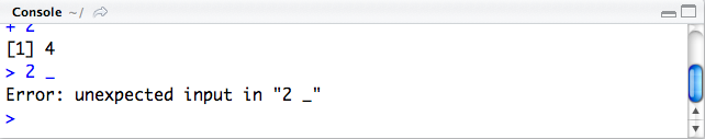
When a command containing an error is issued, RStudio returns the appropriate error message generated by R (Figure 3-2). For the experienced user, these error messages are usually very informative, but for beginning users they may be difficult to interpret.

Many commands involve assignment to a variable. R has two commonly
used options for assignment: = and
← (the latter is preferred by most
longtime R users). The arrow assignment operator has a keyboard shortcut
Alt+- (Option+- in Mac OS X), which makes it as easy to enter as the
equals sign. Using the arrow is recommended—and as a bonus, extra space is
inserted around the assignment operator for clarity.
The Console panel adds very few
actions. As such, there is no toolbar. The current working directory
(getwd) appears in the panel’s title,
along with an arrow icon to open the Files browser to display this directory’s
contents. The Files browser, by design,
does not track the current working directory—but the title bar does, so
this arrow can be a time saver.
The width option (getOption("width")) is consulted by many of R’s
functions in order to control the number of characters per line used in
output. This value is conveniently updated when a user resizes the
horizontal space allocated to the Console. Other options are also implemented to
modify the various prompts, such as prompt and continue.
There are few instances where things can get too long:
- Commands with lengthy output
When the output of a command is too lengthy, it will be truncated. The option
max.printwill be consulted to make this determination. For server usage, one may wish to keep this small, as the data must be passed back from the server to be shown.- Commands with lengthy run times
Sometimes a command will take a long time to execute. This may be by design, but it also can be the result of an erroneous request. In the first case, one can inform the user of the state (e.g.,
?txtProgressBar). In the latter case, a user may wish to interrupt the evaluation. This is done using the Escape key or by clicking on theStopicon that appears during a command’s execution in the right side of theConsolepane’s title bar (Figure 3-3).

Automatic Insertion of Matching Pairs
In R, many characters come in pairs: parentheses, brackets,
braces, and quotes ((, [, [[,
", and '). Failing to have a matching pair will often
result in a parse error or an incomplete command, both annoyances.
RStudio tries to circumvent this by automatically creating matching
pairs when the first one is entered. That is, typing a left parenthesis
adds a matching right one. Also, deleting one will can cause the other
to be deleted if no text is entered in between.
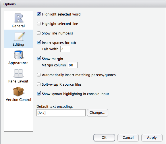
While a useful convenience, this feature can be hard to get accustomed to, so it can be turned off. RStudio’s Options dialog (Preferences in Mac OS X) provides a toggle button (Figure 3-4). Even if this feature is turned off, RStudio still provides assistance with matching pairs by highlighting the opening parenthesis, bracket, or brace when the cursor is positioned at the closing one.
R Script Files
The console is excellent for quick interactive commands but not as
convenient for longer, multiline commands. For such tasks, being able to
type the commands into a file to be executed as a block proves very
useful. Not only is it easier to see the underlying logic of the
commands and to find any errors, this style also allows one to easily
archive commands for later reference. The RStudio Source editor (described more fully in Source Code Editor) can be used for writing scripts and
executing blocks of code from them.
A new R script file can be opened in the code editor using the
leftmost toolbar button on the application toolbar or from the File > New > R Script menu item. Into
this file a series of commands may be typed. There are different actions
available that execute these commands in part or in total:
- Run line or selection
Run the current line or selection. Commands that are run are added to the history stack (Command History).
- Run all lines
Run all the lines in the buffer.
- Run from beginning to line or run from line to end
Run lines above or below the current line including current.
- Run function
Have RStudio look for the function enclosing the cursor and run that.
- Rerun previous region
This allows one to edit a region and rerun its contents without needing to reselect it.
- Source (or Source with echo)
Call
sourceon the file (“source with echo” will echo back the commands). Sourced commands do not add to the history stack.
These actions are invoked via the menu bar, keyboard shortcut, or
toolbar button. All appear under the Edit menu item and have their corresponding
keyboard shortcut shown (Table 3-2). The toolbar buttons
for the editor allow one to run the line or selection quickly, rerun the
previous region, or source the buffer into R.
Command-Line Conveniences
Working with a command line has a long history. Despite the popularity of GUIs, command lines still have many aficionados, as they are more expressive—and, once some conveniences are learned—usually much faster to use. For reproducible research they are great, as they can record the exact commands used. There are drawbacks, though. Typing can be a chore, proper command syntax is essential, and the user needs to have intimate knowledge of the function and its arguments. All of these can be huge obstacles to newcomers to R. Over time, these drawbacks of command-line usage have been lessened through techniques such as tab completion, keyboard shortcuts, and history stacks.
We discuss RStudio’s implementation of these next. Becoming well-versed in these features can help you turn the command line from a distant stranger into a welcome friend.
Tab Completion
Working at the command line requires users to remember function names and the names of their arguments. To save keystrokes, many R users rely on tab completion to complete partially typed commands. The basic idea of tab completion is that when the user has a partially completed command and the Tab key is pressed, the command will be completed if there is only one candidate for completion. If there is more than one, a menu of candidates is given to choose from. The implementation of this feature varies across the different R interfaces, although most implement it—none, perhaps, as intuitively as RStudio. Here the menu provided for candidate selection is a context-sensitive completion dialog raised (when needed) by pressing the Tab key and dismissed by making a selection or by pressing either the Backspace or Escape key.
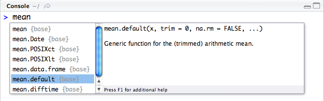
The completion dialog (see Figure 3-5) has a left pane with options that can be scrolled through, and usually a right pane providing details on the selection (if available). This short description is great for jogging memories as to what the value effects. The corresponding help page that contains this information can be opened by pressing the F1 key.
A candidate value for completion may be selected with a mouse, but it is typically more convenient to use the keyboard. Press the up or down arrow to scroll through the list and use the Enter key (or Tab key again) to select the currently highlighted value for insertion. Typing a new character will narrow the list of candidates.
The completion window depends on the context of the cursor when the Tab key is pressed. Here are some scenarios:
- Completion of object and function names
When an object or function name is partially typed, the completion candidates will be objects on the user’s search path whose case-sensitive name begins with the value. Objects may be in the global workspace of the user or available objects from the loaded packages (functions, variables, and data sets). In the latter case, the package name appears next to the value and, when possible, a summary of the object from its help page (Figure 3-5).
- Listing of function arguments
If the cursor is inside the matched pair of parentheses enclosing a function’s arguments and the Tab key is pressed, the arguments will populate the completion candidates (Figure 3-6). The arguments appear with an
=appended to their name, to distinguish them from objects.- Completion within a function’s argument list
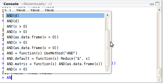
Within a populated argument list, the completion code provides arguments and objects, as both may be desired (Figure 3-7). R can use named arguments or positional arguments where only the object is specified.
- Completion within strings
Within quotes, the completion code will offer a list of files and subdirectories to choose from (Figure 3-8). By default, this will list files and directories in the working directory, but if any part of a path is given (absolute or using the “tilde” expansion) then files and directories relative to that are presented.


Note
The selection of completion candidates is eventually delegated
to a framework provided by R’s utils package and documented under rcompgen. That help page has much more
detail on how the completion candidates are figured out. For example,
completion can be done after the extractors $ (for lists and environments) and @ (for S4 objects). In this case, the
completion window has no details pane. Additionally, completion can be
carried out inside namespaces, even when not exported (using :::).
There are a few limitations of the completion mechanism. Completion of function arguments can be difficult for generic functions, as the argument list may depend on the specified arguments and these are not evaluated; and the token for completion is found by considering the current line, so it doesn’t work well with multiline commands.
Keyboard Shortcuts
Keyboard shortcuts allow the user to quickly invoke common actions by pressing the appropriate keyboard combination. For example, many people have their fingers trained for the copy and paste keyboard shortcuts, as using them can be more convenient than using a mouse to initiate these actions. RStudio has numerous keyboard shortcuts. In keeping with standard GUI design, many of these appear alongside the menu item associated with the action. Here, we discuss those shortcuts that are implemented for the console and its integration with the source-code editor.
Keyboard shortcuts are usually operating-system dependent, and
RStudio’s are no exception (though, they are not locale specific).
Additionally, keybindings may also be editor-dependent. In particular,
the well-established vi and Emacs keybindings are hardwired into many
users’ fingers. The RStudio keybindings are a mix of OS-consistent
bindings (e.g., copy and paste in Windows is Ctrl+C and Ctrl+V, and in
Mac OS X, Cmd+C and Cmd+V) and Emacs-specific (e.g., Ctrl+K will kill
all the text to the right of the cursor [including the end-of-line
character] and Ctrl+Y will yank it back [paste it in]). Although
vi users may feel left out, adding in
the Emacs bindings surely makes many longtime R users happy—it is hard
to retrain one’s fingers! Similar shortcuts have been present for a long
time in R’s console through the readline library.
In Table 1-2, we listed shortcuts for navigation between components. Here in Table 3-1, we describe shortcuts for working at the console, and in Table 3-2 list the available shortcuts for sending commands from the source-code editor to the console. General editing shortcuts for the console and source editor are listed later in Table 5-1.
Note
In RStudio, keybindings are currently not customizable. Keeping
consistency across platforms, the web interface, and the
Qt desktop is difficult. Keyboard shortcuts do
get updated on occasion. The current list is found under the menu item
Help > Keyboard
        Shortcuts
.
| Description | Windows and Linux | Mac |
Ctrl+2 | Ctrl+2 | |
Clear console | Ctrl+L | Command+L |
Move cursor to beginning of line | Home | Command+Left |
Move cursor to end of line | End | Command+Right |
Navigate command history | Up/Down | Up/Down |
Pop-up command history | Ctrl+Up | Command+Up |
Interrupt currently executing command | Esc | Esc |
Change working directory | Ctrl+Shift+K | Ctrl+Shift+K |
| Description | Windows and Linux | Mac |
Ctrl+Enter | Command+Enter | |
Run current document | Ctrl+Shift+R | Command+Shift+R |
Run from document beginning to current line | Ctrl+Shift+B | Command+Shift+B |
Run from current line to document end | Ctrl+Shift+E | Command+Shift+E |
Run the current function definition | Ctrl+Shift+F | Command+Shift+F |
Rerun previous region | Ctrl+Shift+P | Command+Shift+P |
Source a file | Ctrl+Shift+O | Command+Shift+O |
Source the current document | Ctrl+Shift+S | Command+Shift+S |
Command History
Interactive usage often involves repeating a past command or parts of a command. Perhaps one wishes to change an argument’s value, or perhaps there was a minor error. Retyping an entire command to make a minor change is tedious at best. A common instinct is to insert the cursor at the error and edit the previously issued command, but this is not typically supported by console usage. One might then be tempted to copy and paste the command to the prompt and proceed to edit. Though this works, the history mechanism speeds up this process.
RStudio keeps a stack of past commands and allows one to scroll through them easily. This can be done using the up and down arrow keys. As the arrows are pressed, the previous commands are copied to the prompt, allowing them to be edited. The list of commands can be scrolled through quickly.
To see more than one previous command at a time, the Ctrl+Up keyboard shortcut can be typed, and a history window, similar to that for tab completion, will pop up (Figure 3-9).
Searching the history stack
Searching (as opposed to scrolling) through the past history (Ctrl+R on many R consoles) is better for lengthy sessions. RStudio implements searching its own way. Calling Ctrl+Up when there is text already typed at the prompt will narrow the list shown in the history pop up to just commands beginning with that text. One can use the arrow keys or mouse to select a value. Alternatively, one can continue typing, which causes the pop up to close and reopen with a narrowed list.
History Browser
In addition to the command-line interaction
with a user’s history, RStudio also provides a History browser (Figure 3-10), allowing the user to scroll through
past commands or use a search box. The past commands are organized in
time order, with timestamps added for extended sessions. By default,
this component resides in a tab on the upper right, and may be raised
by clicking on the tab or using the shortcut Ctrl+4.
The basic usage involves double-clicking a line, which sends it to the console to be edited or reissued (the focus shifts to the console, so just pressing the Enter key will re-execute the command). Other uses involve first marking a selection. A single click selects the line, and this selection can be extended by holding the Shift key and using the up and down arrows. Other selection modifications are also possible. The component’s toolbar has three buttons: one sends the selection to the console, one appends the selection to a file in the source-code editor (opening one if need be), and one removes the selection from the history list (the page icon with the red “x”). If a multiline selection is sent to the console, no continuation prompt is inserted, allowing one to edit any of the lines.
The toolbar also has icons to save the history to a file, read the history in from a file, and clear the history in its entirety.

The General panel of the options dialog has a couple of entries related to the history-recording mechanism: one to modify how the history is saved and one to toggle the option to remove duplicate commands.
Workspace Browser
When an R user assigns a value to a variable, the assignment is held
in an environment, R’s way of organizing its objects.
Environments are nested, and this nesting is traversed to locate variable
assignments. The user’s global workspace (.GlobalEnv) is the top-level environment where
names are bound during interactive use (Figure 3-11). This workspace is typically
persistent—that is, a user is prompted to save it when quitting an R
session, and it is loaded on startup or when a new project is selected
(see Which Workspace?). Over time, there can be many
variables, and remembering what they are can become nearly impossible. R
has some functions to list the variables in an environment (primarily
ls), but RStudio makes this much easier
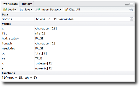
through its Workspace browser.
The Workspace browser appears by
default as a tabbed pane in the upper-right of the GUI. The browser lists
the objects in the global workspace, organized by type of value: Data, Values,
Functions.
Note
The global workspace is not the only environment that R uses.
Indeed, it is just one of many. For example, without extra work, within
a function assignment occurs in the function’s environment and
disappears when the function exits. Such assignments do not appear in
the Workspace browser.
Editing and Viewing Objects
Clicking on a value will initiate an action to edit or view the
object. Currently, rectangular objects, such as data frames and
matrices, are not editable. For these, RStudio provides an
implementation for View (really
dataentry).
For other objects, how the value gets edited depends on the type of object and its length.
For some atomic objects with length 1, the editing occurs within
the Workspace browser (Figure 3-12). Clicking on the object
highlights its value, which can then be edited using the browser as a
property editor. The input expression is not evaluated and need not be
of the same class.
More typically, clicking on an object invokes an editor in a
pop-up window. In Figure 3-13, we
see the editor appearing after clicking on the ch variable, a character vector of length
12.


One can edit and save, or simply cancel. Similarly, one can edit functions through the same editor.
Editing an object involves first deparsing the object into a
file and then calling the editor on that file. When editing is
finished, the text is parsed and, if there is no error, this value is
assigned (see ?edit for details).
Editing of functions preserves the function environment. Editing of
some objects—for instance, S4 objects—is not
possible.
For data frames and matrices, there is a data viewer. Clicking on
such an object will open a view of the data in the code-editor pane
similar to Figure 3-14. At the
time of this writing, the view is limited to 100 columns and 1,000
lines. This view is a snapshot and is not updated if the underlying
object changes. However, reclicking the object in the Workspace browser will
refresh the view.

The Workspace browser has a few
other features available through its toolbar for manipulating the
workspace:
Previously saved workspaces (or the default one) can be loaded through a dialog invoked by the
Loadtoolbar button.The current workspace can be saved either as the default workspace (
.RDatafile) or to an alternate file.The entire workspace can be cleared through the
Clear Alltoolbar button. To delete single items, one can use thermfunction through the console.
Importing Data Sets
Importing data into an R session can be done in numerous ways, as
there are many different data formats. The R Data
Import/Export manual provides details for common cases. For
properly formatted text files, RStudio provides the Import Dataset toolbar button to open a dialog
to initiate the process. You select where the file resides (locally, or
as a web resource), then a dialog opens to select the file. Once a file
is specified (and possibly downloaded/uploaded), a dialog appears that
allows you to customize how the data will be imported. Figure 3-15 shows the defaults for
reading in the mtcars data when first
written out as a csv file.

The dialog has the more commonly used arguments for a call to
read.table, but it is missing a few,
such as comment.char.
Note
For server usage, one can upload arbitrary files into the
working directory through the Files
browser (see The File Browser).
The Help Page Viewer
As mentioned, R is enhanced by external code organized into packages. Packages are a structured means for the functions and objects that extend R. Part of this organization extends to documentation. R has a few ways of documenting itself in a package. For packages on CRAN, compliance is checked automatically. Each exported function should be documented in a help page. This page typically contains a description of the function, a description of its arguments, additional information potentially of use to the user, and, optionally, some example code. Multiple functions may share the same documentation file. In addition to examples for a function, a package may contain demos to illustrate key functionality and vignettes (longer documents describing the package and what it provides).
R has its own format, Rd format, for marking up
its help pages. This format is well described in Writing R
Extensions, one of the manuals that accompanies R. As the
Rd format is structured, functions (in
the tools package) have been written to
convert the text to HTML format. R comes with a local web server to
display these pages. RStudio can show them as well, and does so in its
Help browser. By default, this
component (Figure 3-16) appears in the pane in
the lower-right corner.

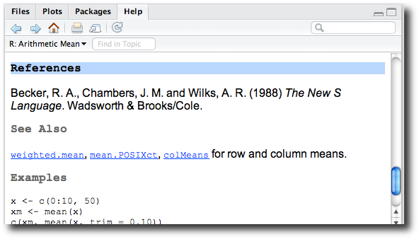
Help pages are invoked by the help function, although the easy-to-type
shortcut ? is typically used. For
example, executing ?mean will open the help page for
the mean function from the base package (Figure 3-16).
An advantage of HTML rendering of help pages is that the provided
links are active. For example, in the mean help page, the help page author provides
links (Figure 3-17) to weighted.mean (for computing a mean with
weights), mean.POSIXct (an S3 method for computing the mean of time data),
and colMeans.
Note
The add-on helpr package for R
enhances the appearance of the help pages by applying attractive CSS
styling, adding a comment feature, and providing the ability to execute
the examples directly from the Help
browser.
The ? shortcut is the most basic
functionality for help. In the Packages pane, the installed packages appear as
a link. Clicking such a link opens a description page for the package (as
would a command like help(package="package_name")). This description
page gives links to the documented functions, and in addition (if
applicable) provides access to the DESCRIPTION file, the NEWS file, a list of demos, and any package
vignettes.
The ?? shortcut allows quicker
access to R’s help.search function.
This allows for searching the help system’s documentation for a match to
the specific pattern, searching within the alias, title, and concept
entries. (The help.search function
allows a more refined search.) As of R 2.14.0, the results are returned in
a search results page in the Help
browser with links to the different matches.
There are two different search boxes provided by the Help browser. The box in the upper-right corner
of the main toolbar (Figure 3-18) lists the
available help topics matching the beginning of the typed expression,
using an auto-completion feature. This serves a similar, but more
convenient, role as the apropos
function, which can be used to search for workspace objects matching a
pattern. The lower search box in the secondary toolbar is used to search
through the contents of the displayed help page.
Note
Searching for text in RStudio is complicated by the presence of the many different panels. Basic search happens through the source-code editor; other searches are facilitated by panel-specific search boxes.

In addition to the search box, the Help browser’s main toolbar provides other
functionality:
The arrows are used to scroll through the history of one’s help-page usage. This history also appears as the values of a pop-up combobox when a help page is shown.
Clicking the “home” toolbar button opens a page providing, among other items, links to the manuals that accompany R.
The
show in new windowtoolbar button will open the page in a web browser.
Searching online resources
R is widely discussed on internet forums and news groups. The
RSiteSearch command is used to search
for key words or phrases from various sources of help that exist online
and in packages, through
http://search.r-project.org. This command opens a
browser window containing the results. The sos package provides an alternative
interface.
Other useful places to find information about R or RStudio are the R mailing lists, the Stack Overflow thread for R at http://stackoverflow.com/questions/tagged/r, and the RStudio support forum at http://support.rstudio.org.
Graphics in RStudio
R, as a computing environment, is well known for its abilities to produce publication-quality graphics. Indeed, R graphics are often seen on the pages of The New York Times. To achieve this quality, the graphics engines in R have many levels of customization. Over the years, R has developed several different engines for producing graphics:
The base graphics system offers easy-to-use statistics-oriented graphs and underlying low-level functions to allow users to design their own.
The
latticepackage implements Trellis Graphics (an implementation of ideas in Visualizing Data, by William S. Cleveland [Hobart Press]) forSandS-Plus. Lattice graphics are very well suited for displaying multivariate data. Many standard statistical plots are easy to make, but an underlying flexibility allows users to create their own graphics.The
ggplot2package provides a relatively recent third approach. This is an implementation by H. Wickham of ideas in The Grammar of Graphics by L. Wilkinson, et al. (Springer). It advertises that it combines the advantages of base and lattice graphics—in addition, it produces very attractive graphics. Again, one can quickly generate stock graphs, but there is much flexibility to build up a graph step by step.
All three of these systems rely on R’s underlying graphics
framework. R uses a paper-and-pen approach to graphics. A graphic device
(the paper) is created or cleared, and the graphic commands then write
(with pen) onto this paper in steps. The point of this analogy is that one
can’t erase the paper. (The cranvas
package will provide an alternative to this, but that is a different
topic.) As such, it is important to plan a graphic prior to creating
it—for example, computing the size of the coordinate space that will be
needed. (Don’t worry, this is usually done for you by the calling
function.) The device (or piece of paper) is quite flexible in general. It
can be an interactive device or a device that writes to a file in a
certain format, such as pdf,
png, or svg.
Note
Don’t be turned off by the apparent complexity hinted at above.
Although both the lattice and
ggplot2 packages are documented in
book-length formats, this only reflects their underlying flexibility.
All three graphics approaches provide enough higher-level functions that
make the standard graphics of statistics as simple as remembering the
function name and specifying the data appropriately.
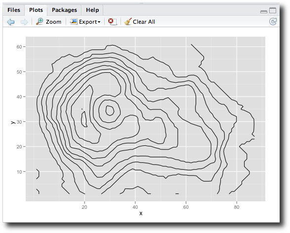
The Plots Browser
RStudio provides its own device for the display of graphics,
RStudioGD. By default, the device’s
output is rendered in the Plots
browser. Although the graphics are secretly image files, the RStudioGD device also allows for
interactivity. In Figure 3-19 we see a graph
from one of the examples of stat_contour from ggplot2 displayed in the browser.
The image is initially sized to fit the space allocated to the
browser. If the browser is resized, the image will be regenerated to
match the new size. This happens in the background, though there is a
button to refresh the current plot on the component’s toolbar. If one
desires an even larger view, the zoom
toolbar button will open the graphic in a much larger Plot Zoom pop-up window. The zoom window is
not an interactive device but a snapshot of the current graphic.
One benefit of how the device works is that a new graphic is produced each time (unlike many R devices, which essentially have an erase feature). This makes it easy for the component to keep a list of the graphics that are produced. One can scroll through old graphics using the left and right arrows located on the toolbar.
The currently viewed graphic can be exported as an image or .pdf file. RStudio provides a few dialogs to control this. In Figure 3-20, we see that the save-plot dialog allows one to easily specify the file type, directory, and file name of the image, as well as adjust the size of the image in pixels. The size can be adjusted by entering a value, or by dynamically adjusting the size with the grab handle in the lower right.

In addition, there are toolbar buttons to remove the current plot and to clear all the plots.
Interactivity
R allows for interaction with a graphic through the locator function, which returns the position
of the point (in the “user coordinate system”) where the (first) mouse
button is pressed; and the identify
function, which returns the index of the point nearest to where the
(first) mouse button is pressed. Both functions are implemented for the
RStudioGD device.
When the functions are called, the Plots browser is raised (if it wasn’t
already). The two functions are blocking, in that no input into the
console is available until after the selection of coordinates is done.
The console shows its stop icon, and the graphic device displays a
message (Figure 3-21) that the locator is
active, and instructs the user to press the Finish button. (For locator, one specifies ahead of time the
number of points to identify, so the block will terminate if that occurs
as well.)

Note
Some devices for R implement more complicated events, through
getGraphicsEvent, but this is not
currently the case for the RStudio
device.
The manipulate Package for RStudio
Through the tcltk package (and
others), an R programmer can create graphics that can have associated
GUI controls to manipulate the display. Through the manipulate package, RStudio users can too.
This package is provided with RStudio and delivers a set of
simple-to-define controls that provide values to an expression used for
plotting. These controls include a button, a slider, a picker, and a checkbox.
The basic usage is:
One defines an expression that, when evaluated, produces the desired plot.
This expression includes parameters labeled with the names given to the controls.
When a control is updated, the expression is reevaluated and the graphic updated.
To illustrate, Figure 3-22 shows
the code that implements the tkdensity demo from the tcltk package (there are 103 lines in the
original, but just 16 here).
When the commands are executed, RStudio produces a plot based on the initial values of the control and also pops up a window with the controls as shown in Figure 3-23). Manipulating these controls will update the graphic (but not add to the history of graphics). The control frame’s visibility is toggled through the double arrow icon in the control bar and the gear icon in the plot window.
This example shows three control types. A slider appears with both its own label, another label indicating the value, and a slider widget to adjust that value. The pickers are rendered using comboboxes, and the checkbox is displayed with its accompanying label.


External Programs (Desktop Version)
R has several packages that provide interfaces to external programs
and systems. For the desktop version of RStudio, in many cases one can
call these to extend the interface (though such interactions can be
temperamental.) For example, the tcltk
package interfaces R with the Tk
libraries for creating graphical user interfaces. The widely used Rcmdr package uses this package to provide a set
of graphical interfaces to numerous R functions. The use of the tcltk package, as well as others such as
RGtk2 and rJava, can be a little inconsistent under
RStudio—though in many setups, they will work.
In addition, the desktop user can take advantage of R’s internal
help server. The package googleVis uses
this to display Google’s visualization tools in a browser. The Rook package provides an API for R users to
write web applications that take advantage of this same server.