To organize our work, we set up a new project (see the section Organizing Activities with Projects). RStudio allows us to compartmentalize our work into projects that have separate global workspaces and associated files and integrate seamlessly with version control systems. We easily navigate between projects using a selector (a combobox) in the main toolbar located in the upper-right corner. The same selector has an option to create a New Project..., which we choose. To create a new project, one fills in a project name and location, and if available, one can specify if version control is to be used.

When the project is created, the working directory is set. The title bar of the Console pane is updated, as are the contents of the Files component, which lists the files and subdirectories in a given directory. The Files pane resides by default in the lower-right corner. If it isn’t showing, select its tab. In Figure 2-1, we see that our working directory contains our data file and a bookkeeping file written when RStudio created the package.

Figure 2-1. The Files browser shows files added when a new project is created

The Files browser pane is typical of RStudio’s components. In addition to the main application toolbar, most components come with their own toolbar. In this case, the toolbar has buttons to add a new folder, delete selected files, etc. In addition, the Files component adds a second toolbar to facilitate the selection of files and navigation within directories.

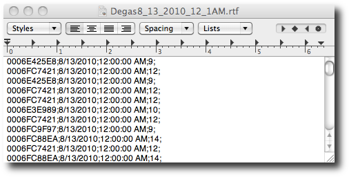
Clicking on the data file name in the file browser opens up a system text editor (Figure 2-2), allowing us to edit the file. For many text-based files, the file will open in RStudio’s source-code editor. However, the actual editor employed depends on the extension and MIME type of the file. For rtf files, the underlying operating system’s editor is used, which for Mac OS X is textedit. We can see that the data appears to have one line per record, with the values separated by semicolons. The fields are RFID, date, time, and gate number. This is basically comma-separated-value (CSV) data with a nonstandard separator.

Figure 2-2. The rtf file is opened in an editor provided by the system, not by RStudio

However, although we rarely see rtf files, we know the textedit program of Mac OS X will likely render them using the markup for formatting, so perhaps there are some markup commands that need to be removed. To investigate, we make a copy of the data file, but store it instead with a txt extension. The Files component makes it easy to perform basic file operations such as this. To make a copy of a file, one selects the checkbox next to the file and invokes the More > Copy… menu item, as seen in Figure 2-3.

Figure 2-3. Copying files in the Files browser—the command acts on the checked file

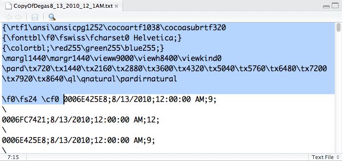
We change the extension to txt and our file list is updated. (In general this can be a really bad practice, especially for binary files, though in this case we know rtf files can be viewed as plain text.) The displayed contents of the directory may also be refreshed by clicking the terminus on the path indicated by the links to the right of the house icon in the secondary toolbar; or the refresh icon on the far right of the component’s main toolbar. Now, clicking on the txt file opens the file in RStudio’s source-code editor as a text file (Figure 2-4).

The editor’s status bar shows us the line and position of the cursor and, on the far right, that we are looking at a text file. We can now see that there is indeed a header (and, if we scroll down, a footer) wrapping our data. We highlight the header and then use the Delete key to remove this content from the file. We then scroll to the bottom of the file and remove a trailing brace. Afterwards, we click the Save toolbar button (the floppy-disk toolbar button, which is grayed out in the figure, as no changes have been made).

Figure 2-4. RStudio’s code editor showing actual contents of our data file; we need to delete the rtf formatting before reading in

We now wish to read in the file using read.csv. RStudio provides an Import Dataset toolbar button under the Workspace component, which provides an interface that will handle most csv data, such as that exported from a spreadsheet. In this example though, we have a few idiosyncrasies that prevent its use. (This is a deliberate choice to show off some of RStudio’s other features.)

So we head on over to the Console component to do the work. With the default pane arrangement the console is located on the left side (the lower-left pane if the editor is open). In R, one can’t avoid the console, and RStudio’s should look very familiar to any R user.

At the console we create the command to call the read.csv function directly. This requires us to specify a few of its arguments, as we have a different separator, an odd character every other line, and no header. We will use the tab completion feature to assist us in filling in these values. This feature provides completion candidates for many different settings, allowing us in this case to recall quickly the names for lesser-used arguments.

First, we type read.csv in the console. Then we press the Tab key to bring up the tab completion dialog (Figure 2-5) for this function.

Figure 2-5. Tab completion dialog showing small snippet about the read.csv function from the function’s help page

RStudio’s tab completion dialog for a function nicely displays its arguments and a short description, gleaned from its help page (when available). In this example we see the sep argument is what we need to specify a semicolon for a separator, the header argument to specify a non-default header, and comment.char to skip the lines starting with a backslash.

The file name is the first argument. For file names (indicated by quotes), tab completion will fill in the file name, or, if more than one candidate is possible, provide a popup (Figure 2-6) to fill in the file. Here we type a left parentheses and double quote, and RStudio provides the matching values.

Figure 2-6. Tab-key completion for strings; a list of files is presented

We press the Tab key again to select the proposed completion value using our modified text file, not the original. We then add a comma and again press the Tab key. When the prompt is in a function body, the tab completion will prompt for function arguments. After entering our values, we have this command to issue (see also Figure 2-7, where the command is shown in the console):

> x <- read.csv("CopyOfDegas8_13_2010_12_1AM.txt", sep=";",
+ header=FALSE, comment.char="\")

Figure 2-7. Command to read the “csv” file holding the data within the RStudio console

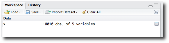
The Workspace component lists the objects in the project’s global workspace. In the default pane layout, this component is in the upper-right pane along with the History component. If this pane isn’t raised, we simply click on its tab (or perform the keyboard shortcut Ctrl-3) to do so. After the data is read in, this component is updated to reflect the new object, in this case one named x (Figure 2-8). The associated icon for x shows it to be rectangular data. Clicking on x’s row invokes the View function on x—in this case, opening the data viewer (Figure 2-9).

Figure 2-8. Workspace browser showing a data object x

Figure 2-9. Data viewer window showing non-editable display of the x data frame

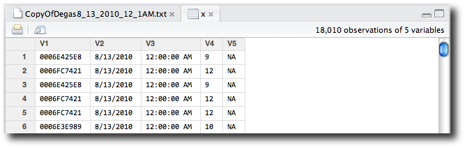
The data viewer shows us that we have an unnecessary fifth column of NA values, and that our variable names need improvement. Although the data viewer of RStudio does not yet support editing, R has many ways to manipulate rectangular data at the command line. For our two tasks we issue the following:

> x <- x[ , -5]
> names(x) <- c("RFID", "date", "time", "gate")

The view of x in the code-editor pane does not update from changes at the command line; rather, it is a snapshot. The Workspace component does reflect the current state of the variable, and reclicking on that will refresh the view.

Using the Right Class to Store Data

The data is time-series data, but the date and time are read in and stored by read.csv as factors, not times. R has many different classes for working with time-series data. In this case study we will look at two. The POSIXct class records time by the number of seconds since the beginning of 1970 and is useful for storing times in a data frame, such as x. We will use the coercion function as.POSIXct for this task. As this function isn’t part of our daily repertoire, we call up its help page. Opening a help page can be done in the standard way: ?as.POSIXct (Figure 2-10).

Figure 2-10. Help page for the POSIXct function

Help pages are displayed in the Help pane, located by default in the lower-right corner. RStudio’s help browser also has a search box on the upper right of its main toolbar to locate a help page, or the page can be opened with tab completion and the F1 key. Due to its web-technology roots, RStudio easily leverages R’s HTML help system; pages appearing in the Help pane have active links.

After consulting the help page, we see that the format argument is needed. This specification is described elsewhere, in the help page for the strptime function. Clicking on the provided link opens that page, allowing us to figure out that the specification needed to make our function call is:

> x$datetime  <- paste(x$date, x$time)
> x$time <- as.POSIXct(x$datetime, format="%m/%d/%Y %H:%M:%S")

At this point we have a data frame, x, storing all the information we have about the colony of mole rats. However, the data set needs to be cleaned up, as there are some repeated observations. We do this on a per-rat basis. R has several ways to implement the split-apply-combine idiom, as it is one of the most useful patterns for R users. The plyr package is widely used, but for this task we use functions from base R. The split function can be used to divide the data by the grouping variable RFID, returning a list whose components are the records for the individual mole rats:

> l <- split(x, x$RFID)

The list, l, has a different component for each mole rat. We can check to see if any two rows for a mole rat are identical, using R’s convenient duplicated method. In addition, we add a bit of time to to each time value, so that times recorded with the same second are distinguished. R has several different means to apply a function to pieces of an object. Below we use lapply to apply a function to each component of the list l, returning a new list l1 with the modified data:

> l1 <- lapply(l, function(x) {
+  trimmed <- x[duplicated(x),]
+  nr <- nrow(trimmed)
+  trimmed$time <- trimmed$time + seq_len(nr)/nr*(1/1000)
+  trimmed
+ })

The data is recorded by gate, but the actual item of interest is the bubble (chamber) the mole rat is in at a given time. This information allows us to consider how social an animal is by looking at the time shared with others. We need to deduce this information from the data.

We do so by assuming that if the mole rat is in bubble 5, say, and we record gate 5, then the mole rat moved to bubble 6. Or, if the recording was gate 4, then the mole rat moved to bubble 4. (There are 15 bubbles and 14 gates, so gate i is between bubbles i and i+1.) To create the bubble count, we assume the mole rat moves immediately to the bubble after crossing a gate. This ignores the possibility of the mole rat changing its mind and never actually going to the next bubble. We will use a for loop to do this computation.

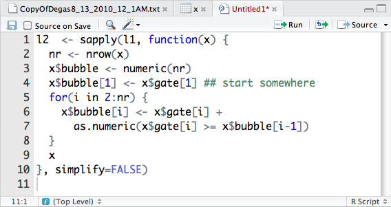
The actual command we need for this computation is a bit long to type in correctly at the command line. We will instead use a script file so we can freely edit our commands. RStudio makes it easy to evaluate lines from a script file in the console. In addition, with the aid of syntax highlighting and automatic code formatting, we can quickly identify common errors before evaluation.

The “open a new R Script file” action is proxied in several places: through the leftmost toolbar button in the application toolbar, through the File > New > R Script menu item, or through a keyboard shortcut (Ctrl+Shift+N). However invoked, once done, a new untitled file appears in the code-editor. In this new file we type in our commands, as shown in Figure 2-11. The figure also shows how the code editor component is used in many ways: to look at raw data sets, view rectangular data objects from the workspace, and edit R commands.

Figure 2-11. Using the source-code editor for multiline commands

With the commands typed in, we are ready to execute them. RStudio allows several variations on how to send the contents of a file to the console. In this case, we simply click on the Source toolbar button at the far right of the pane’s toolbar to call source on the active document.

Each component of the l2 list contains records for a mole rat. The key variables are the times, stored as POSIXct values and bubble. It will be more convenient to use another of R’s date-time classes to represent the data, as then many desirable methods will come along for free. Our data is an irregular time series, as time is marked by mole rat events, not regular intervals on the clock. The zoo package is designed for such data, as one needs only ordered observations for the time index.

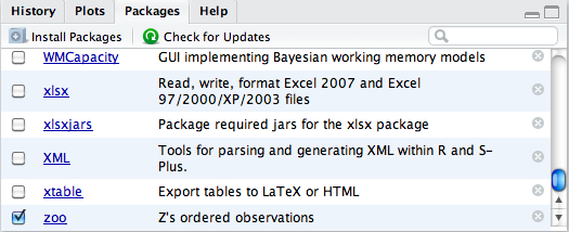
To convert our data into zoo objects, we first need to load the package. RStudio makes working with packages easy through the Packages component, which for us appears in the lower-right pane. Loading or unloading a package is as simple as checking the package’s accompanying checkbox to indicate the desired state (Figure 2-12), where a check indicates the package is loaded.

We had previously installed the zoo package, so it shows in the packages list. Were that not the case, we could have quickly installed the package from CRAN, along with any dependencies, using the dialog raised by clicking the leftmost Install Packages toolbar button in the pane’s toolbar.

Figure 2-12. The Packages component allows you to select packages to load or unload and conveniently provides links to their documentation

To create a zoo object, we call its same-named constructor. The first argument is the data; the second the value to order by. We then merge the data into one zoo object. Here, we also use the na.locf function to carry the last bubble forward to replace an NA when the data is merged:

> l3  <- sapply(l2, function(x) zoo(x$bubble, x$time), simplify=FALSE)
> x  <- na.locf(do.call(merge, l3), na.rm=FALSE)

One of the reasons we used a zoo object is its convenient plot method. We begin by making time series plots of the first five mole rats on the same graphic. We can’t recall the specific arguments, so again let tab completion (Figure 2-13) lead us to the correct help page. In this case we type plot, and the function completion shows us the various plot methods available. Scrolling through, we find plot.zoo.

Figure 2-13. Using tab-key completion to find arguments to the plot method of zoo objects

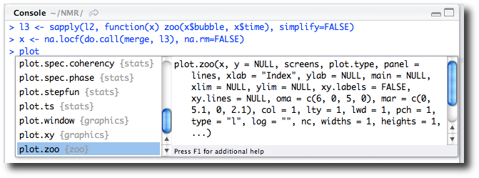
In the figure we see the plot.type argument for this plot method but don’t recall the values to specify the graphic we desire. As instructed, we press the F1 key to call up additional help in the help browser and read that "single" is the desired argument value.

After we issue the command:

> plot(x[, 1:5], plot.type="single")

the Plots component is raised, showing the plot.

Command History

Noting that the individual paths are hard to distinguish once they’ve crossed, we want to add colors to the graphic. The col argument is used for this. Rather than retype the previous command, we can edit it. RStudio keeps a record of previous commands. The up and down arrow shortcuts can be used to scroll through our command history. For more complicated usage, we can use the History component, which allows us to browse the past commands and reissue them. We use the up arrow for this case, then modify the col argument to a simple value of 1:5, producing Figure 2-14.

Figure 2-14. The Plots component showing a time-series plot of the first five cases

The plot is sized to fill the Plots pane, and can be on the small side. (Unlike most interactive R use, where the plot devices choose their size.) Often this is all that is needed, but in this particular case we wish it to be bigger. The Zoom toolbar button of the Plots component’s toolbar will open the graph in a larger window.

At this point, with the help of RStudio, we have completed the data preparation needed for subsequent analysis. We have a zoo object holding all the data (x) and a list of zoo objects (l3) storing data for individual rats. In the process of this 30-minute analysis, we took advantage of most all of RStudio’s key components: the Files browser, tab completion, the text editor, the Help browser, the rectangular data viewer, the Console, the Source code editor, the Packages browser, and the Plots viewer.