10 Topic modeling

This chapter covers

• Introducing topic modeling with latent Dirichlet allocation
• Exploring gensim, an NLP toolkit for topic modeling
• Implementing an unsupervised topic modeling approach using gensim
• Introducing several visualization techniques for topic exploration in data

The previous chapter introduced various NLP and machine-learning techniques for topic classification and topic analysis. Here is a reminder of the scenario that you’ve worked on: suppose you work as a content manager for a large news platform. Your platform hosts texts from a wide variety of authors and mainly specializes in the following set of well-established topics: Politics, Finance, Science, Sports, and Arts. Your task is to decide, for every incoming article, which topic it belongs to and post it under the relevant tab on the platform. Here are some questions for you to consider:

1. Can you use your knowledge of NLP and machine-learning algorithms to help you automate this process?

2. What if you suspect that a new set of yet-uncovered topics, besides the five just mentioned, started emerging among the texts that authors send you (e.g., you get some articles on the technological advances)? How can you discover such new topics and include them in your analysis?

3. What if you think that some articles lend themselves to multiple topics, which are covered by these articles to a various extent? For instance, some articles may talk about a sports event that is of a certain political importance (e.g., Olympic Games) or about a new technological invention that results in the tech company having high valuation.

Let’s summarize what you have done to address the tasks in this scenario so far:

• First of all, as question 1 suggests, you can apply your NLP and ML skills and treat this task as another text classification problem. You’ve worked on various text classification problems (spam detection, authorship profiling, sentiment analysis) before, so you have quite a lot of experience with this framework. The very first approach that you can apply to the task at hand is to use an ML classifier trained on the articles that were assigned with topics in the past, using words occurring in these articles as features. As we said in the previous chapter, this is simply an extension of the binary classification scenario to a multiclass classification one. In the previous chapter, you worked with the famous 20 Newsgroups dataset (accessed via scikit-learn at http://mng.bz/95qq) and since you focused on ten specific topics in this data, the first approach that you applied was indeed a supervised ten-class topic classification approach.

• The results looked good, but there are several drawbacks to treating this task as a supervised classification problem. First of all, it relies on the idea that high-quality data labeled with topics of interest can be easily obtained, which is not always the case in real-life scenarios. Second, this approach will not help you if the data on the news platform changes and new topics keep cropping up, as question 2 outlines. Third, it is possible that some texts on your platform belong to more than one topic, as question 3 suggests. In summary, all these drawbacks can be said to be related to availability of data and appropriate labels. What can you do if you don’t have enough annotated data, or you cannot keep collecting and annotating data constantly, or you don’t have access to multiple topic labels for your articles? The answer is you can use an unsupervised machine-learning approach. The goal of such approaches is to discover groups of similar posts in data without the use of predefined labels. If you have some labeled data, you can compare the groups discovered with an unsupervised approach to the labeled groups, but you can also use the unsupervised approach to get new insights.

• The unsupervised approach that you looked into in the previous chapter is clustering. With clustering, you rely on the inherent similarities between documents and let the algorithm figure out how the documents should be grouped together based on these similarities. For instance, in the previous chapter you used K-means clustering (with k = 10 for 10 topics in your data), and the algorithm used word occurrences in the newsgroups posts as the basis for their content similarity. Since this approach is agnostic to the particular classes that it tries to identify, it helped you to uncover some new insights into the data. For example, certain posts from originally different topics (e.g., on baseball & hockey or on autos & motorcycles) were grouped together, while certain posts originally from the same topic were split into several clusters (e.g., forsale turned out to be one of such heterogeneous topics with posts that can be thought of as representing different subtopics depending on what is being sold).

Unsupervised approaches such as clustering are good for data exploration and uncovering new insights. One aspect not addressed by this clustering algorithm is the possibility that some posts may naturally cover more than one topic. For example, a post where a user is selling their old car falls into two categories at once: forsale and autos. In this chapter you will learn how to build a topic modeling algorithm capable of detecting multiple topics in a given document using latent Dirichlet allocation (LDA).

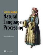
The diagram in figure 10.1 is a reminder of the full set of approaches that you can apply to analyze topics in your data. The two approaches on the left and in the center of this diagram were covered in the previous chapter, and topic modeling is the focus of this chapter.

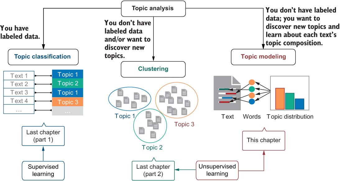
Figure 10.1 Reminder: depending on whether you have labeled data or not, you can apply a supervised (classification from the previous chapter) or an unsupervised approach (e.g., you can use clustering, as discussed in the previous chapter). If you want to discover new topics and learn about text’s topic composition, apply topic modeling from this chapter.

10.1 Topic modeling with latent Dirichlet allocation

The results that you achieved using an unsupervised approach in the previous chapter revealed at least one mixed topic: misc.forsale. This shouldn’t come as a surprise. Despite the fact that all posts where users were selling something ended up in one category within the newsgroups (and similarly might also be posted on the same web page on your online platform), users may be selling all sorts of things, from sports equipment to electronic devices to cars. Therefore, depending on the subject of the sale, a particular post may mix such topics as forsale & baseball, or forsale & electronics, or forsale & autos.

Let’s use some concrete examples. Imagine you have the set of short posts from figure 10.2 in your collection.

Figure 10.2 Examples of short posts on various topics

Let’s discuss the solution to this exercise together.

10.1.1 Exercise 10.1: Question 1 solution

When solving this task, you may follow a procedure like this, which wouldn’t even require you to analyze the meaning of the words, only their occurrence. You start with Post 1, which contains such words as car, accelerate, and seconds, among others. You assign Topic 1 to this post, with the set of words from Post 1 associated with this topic.

Next, you move to Post 2 . Can it also be on Topic 1? Nothing suggests that, as the set of words from this post (hurry, low, price, deal, etc.) don’t overlap with the set that you’ve associated with Topic 1, so you conclude that at this point it would be safest to assign Topic 2 to this post, with the set of words from Post 2 associated with Topic 2.

You move to Post 3 and spot that there is some word overlap with Post 1 and Topic 1—specifically, both posts talk about cars. You decide that Post 3 also belongs to Topic 1. Similarly, Post 4 has some word overlap (specifically, the word price) with Post 2 and Topic 2, so you decide that Post 4 belongs to Topic 2.

Finally, you move to Post 5. Is it on Topic 1 or on Topic 2? On the one hand, it is similar to the posts on Topic 1, as it contains such words as 6-cylinder and engine. On the other hand, it is also similar to the posts on Topic 2, as it contains the word sell(ing). However, the task description says that posts may actually belong to both topics at once. It looks like your original assignment works quite well for this set of posts, as there are no doubts about how the words are distributed among the two topics, and how topics are assigned to posts. This means that at this point you can declare that the topic distribution in these posts is as follows:

• Post 1 and Post 3 are on Topic 1 exclusively.

• Post 2 and Post 4 are on Topic 2 exclusively.

• Post 5 mixes Topic 1 and Topic 2 in some proportion.

Figure 10.3 visualizes this idea.

Figure 10.3 Based on the word composition of each post, Posts 1 and 3 are on Topic 1 exclusively, Posts 2 and 4 are on Topic 2 exclusively, and Post 5 combines two topics in some proportion.

Now you can also list the words that characterize each of these topics:

• Topic 1 can be characterized by car, accelerate, 6-cylinder, engine, model, and so on.

• Topic 2 can be characterized by deal, sell, $, price, and so on.

Can you tell what these topics actually are? Based on the sets of words, you can interpret Topic 1 as autos, and Topic 2 as sales.

10.1.2 Exercise 10.1: Question 2 solution

The algorithm for topic modeling that you will develop in this chapter will follow a procedure similar to the one described earlier: it will start with some topic assignment for the texts, learn about word composition of each topic, and then it will reiterate and update its topic-to-text and word-to-topic assignments to refine its predictions until it reaches the most stable allocation. We will delve into the details of this algorithm in the next section, and now let’s just summarize that the goal of the approach that you will develop in this chapter—the approach that will help you to automatically solve the puzzle—would be to provide you with an answer along the lines of the following:

• Post 1 and Post 3 are 100% on Topic 1.

• Post 2 and Post 4 are 100% on Topic 2.

• Post 5 is on a mix of topics (e.g., 70% on Topic 1 and 30% on Topic 2).

When it comes to the word content, it is also desirable that such an algorithm tells you something like this:

• The composition of Topic 1 is 20% car, 15% engine, 10% speed, 5% accelerate, and so on.

• The composition of Topic 2 is 40% sell, 10% deal, 5% price, 5% cheap, and so on.

To visualize this idea, figure 10.4 illustrates some words that may contribute to each topic using word clouds, where the font size represents the relative weight (i.e., the percentage contribution) of each word within each topic.

Figure 10.4 Sample word clouds representing each of the two topics: the font size represents the relative weight or contribution of each word to each topic.

The exact contribution of the words to the topics will be detected by the algorithm based on the texts. Hopefully this small example helps you appreciate the potential of the unsupervised topic modeling algorithm that you will develop and apply in this chapter: latent Dirichlet allocation (LDA) allows you to interpret texts as combinations of topics that have produced the words that you see in your texts. Specifically, it allows you to quantitatively measure the allocation of topics and the contribution of each word to a particular topic used in your texts. Now it’s time to look more closely into the inner mechanisms of this approach that allow it to come up with such estimations.

10.1.3 Estimating parameters for the LDA

The LDA algorithm treats each document (text, post, etc.) as a mixture of topics. For example, in exercise 10.1, such mixtures contain 100% of Topic 1 in one case, 100% of Topic 2 in another, and 70% of Topic 1 and 30% of Topic 2 in the third case. Each topic, in its turn, is composed of certain words, so once the topic or topics for the document are determined, these topics become the driving forces that are assumed to have produced the words in the document based on the word sets these topics comprise (e.g., {car, engine, speed,...} or {deal, sale, price,...}).

Note In the context of topic modeling, the term document is widely used to denote any type of text (an article, a novel, an email, a post, etc.). We’ll be using this term in its general meaning here too.

This is the theoretical assumption behind LDA—the words that you observe in documents are not put together in these documents in a random manner. Rather it is believed that these words are thematically related, as in exercise 10.1, where some are related to autos and others to sales. All you can observe in practice are the words themselves, but the algorithm assumes that, behind the scenes, these words are generated and put together in the documents by such abstract topics. Since the topics are hidden from the eye of the observer or, to use a technical term, they are latent, this gives the algorithm its name. The goal of the algorithm, then, is to reverse-engineer this document-generation process to detect which topics are responsible for the observed words.

The algorithm focuses on estimating two sets of parameters—topic distribution in the collection of documents and word distribution for each topic on the basis of the documents in the collection. These two sets of parameters, as you will see in the course of this chapter, are very closely related to each other. Just like in exercise 10.1, if the algorithm decides upon the topics (e.g., that Post 1 is entirely on Topic 1), then the words from the document are assigned to this topic, which means that the next time the algorithm encounters any of these words in another document, they will suggest that the other document is on the same topic. Exercise 10.1 explained this process using a small example. It worked well because the set of posts was small, with some word overlap to make things easier, with clear allocation of posts to topics, and only a single post where both topics were present. In a real document collection, there may be thousands of documents with millions of words and many more complex topic combinations. How does the algorithm deal with this level of complexity?

The answer is the algorithm starts with the best possible strategy for the cases where the correct answer is not readily available—namely, it starts by making random allocation. Specifically, it goes through each document in the collection and randomly assigns each word in this document to one of the topics (e.g., Topic 1 or Topic 2). Note that random allocation of words to topics within each document allows the algorithm to account for the possible presence of multiple topics in the same document. Random allocation is widely used as the first step by unsupervised algorithms. You may recall that you also had to randomly allocate documents to clusters in the first iteration of clustering in the previous chapter. Of course, it is unlikely that the algorithm would manage to guess the “right” topics randomly, but the good news is that after this first pass, you have an initial allocation and therefore you can already estimate both the topic distribution in the collection of posts and the word distribution in each topic based on this random guess. Since this guess, being random in nature, will likely not fit the real state of affairs (i.e., the actual underlying distribution), how can you do better?

You apply an iterative algorithm, adjusting the estimation in the “right” direction until your estimation is as good and as stable as possible. At this point, you may recall that the unsupervised clustering algorithm used a very similar procedure. You started with a random cluster allocation, and you kept improving the clusters iteratively until you either have run through the data a sufficient number of times (i.e., you’ve reached the maximum number of iterations) or your cluster allocations didn’t change anymore (i.e., you’ve reached convergence on your solution). The algorithm that you apply here is inherently quite similar in this regard. The key difference is that, instead of one set of parameters, in this case you need to estimate two, taking into account that the topic structure (i.e., the topics themselves, their distributions in documents, and word-to-topic assignments) is a hidden structure, and this structure will need to be estimated and adjusted on the basis of the only observed parameter (i.e., words in documents). Recall that as you are using an unsupervised procedure, the algorithm doesn’t have access to any predefined topic labels and doesn’t know what the “correct” allocation of topics and words is. Let’s summarize the steps in the algorithm. Figure 10.5 provides the mental model for the LDA.

Figure 10.5 Mental model for the LDA algorithm. As in any iterative process, you start with some initial allocation and iterate on your estimates until you do not observe any significant change to the parameters anymore (i.e., until convergence) or until you reach the maximum number of iterations.

Here is a short description of all the steps in the algorithm:

• Step 1: Random allocation—Randomly assign words in documents to topics.

• Step 2: Initial estimation—Estimate topic and word distributions for your data based on the random allocation from step 1.

• Step 3: Reallocation—Evaluate your algorithm on the data, using the distributions estimated in step 2, and reallocate the words to the respective topics accordingly.

• Step 4: Re-estimation—Using the allocation from step 3, re-estimate distributions.

• Iteration—If the new estimates are not considerably different from the previous estimates, stop. Otherwise, repeat steps 3 and 4, until the difference is negligible (i.e., the algorithm converges to a stable solution).

• Stopping criteria—You stop either when estimates stabilize or when the maximum number of iterations has been reached.

How does this process apply to the documents, topics, and words in the topic-labeling application? Suppose on your first pass through the data you have randomly ascribed words to topics. For example, you have 100 words in the post d₁, and for each word in this post you randomly assigned it either to Topic1 (for better readability, you can think of Topic1 as some specific one, such as autos, but keep in mind that the algorithm itself doesn’t “know” what the topic label is) or to Topic2 (again, think of this topic as some specific one, such as sales). Now let’s pass through the data again (step 2) and estimate topic and word probability distributions. In each case, we will first look into the formal definition, then into the calculation, and finally, we’ll consider a toy example.

• Topic probability distribution—The probability of a specific topic t for a specific post d is estimated as the number of words in the post d that have been allocated to the topic t in the previous round of the algorithm application divided by the total number of words in d. In other words, it is

P(topic t | post d) = number of words in post d allocated to topic t / total number of words in post d 

For example, if in the first random pass you randomly assigned 52 words in post d₁ to Topic1, at this point you would estimate that P(Topic2 | d₁) = 0.48 and P(Topic1 | d₁) = 0.52.

• Word probability distribution—The probability of a particular word w, given that a specific topic t produced it, equals the number of times the word w was assigned with the topic t in the previous round in all posts in the collection divided by the total number of times this word has been used in the collection. In other words, it is

P(word w | topic t) = number of times word w is assigned to topic t in all posts in the collection / total number of occurrences of word w 

For example, suppose you’ve encountered the word price 50 times in your collection of posts, 35 of which you have randomly assigned to Topic2 in the first round and 15 of which you’ve assigned to Topic1. This means that P(price | Topic2) = 0.70 and P(price | Topic1) = 0.30.

• In the next pass over the data, you start with d₁ again, and it’s time to reconsider your allocation with topics in this post. Suppose in the previous round you have randomly assigned price to Topic1. Should you change your allocation in view of the new estimates? To decide, multiply the following probabilities:

Pupdate(price is from Topic2) = Pprevious(Topic2 | d1) * Pprevious(price | Topic2) = 0.48 * 0.70 = 0.336, and 
Pupdate(price is from Topic1) = Pprevious(Topic1 | d1) * Pprevious(price | Topic1) = 0.52 * 0.30 = 0.156 

Based on these estimates, since the probability of price being generated by Topic2 in d₁ is higher than the probability of price being generated by Topic1 (0.336 > 0.156), you should change the allocation of price in d₁ to Topic2. Note that even though post d₁ is currently more likely to be on Topic1 overall (since P(Topic2 | d₁) = 0.48 and P(Topic1 | d₁) = 0.52), you are still able to reassign price to Topic2. This is because the distribution of the word price with respect to its topic allocation across all posts matters, too. Moreover, when re-estimating probability for a specific word (e.g., price), you keep other word probabilities as they are (i.e., probabilities for each word are re-estimated separately). This is done so that you don’t need to change too many parameters at the same time, which would make estimation very complex. (A popular algorithm used to make sure the computation is done in a feasible way is based on sampling and is widely used in LDA. For more details, see Resnik and Hardisty (2009), Gibbs Sampling for the Uninitiated, http://mng.bz/j2N8).

• Now that the allocation of some words has changed, you need to pass over your data again, this time re-estimating topic probabilities.

• After multiple passes over the whole collection and re-estimation of topic assignment for all words and then distribution of topics, you will eventually reach a stable distribution where your topic assignments won’t change anymore. At that point, you will be able to use these assignments to detect topic mixtures for each post in the collection by counting the proportion of words in this post belonging to each topic, just like you did earlier. Moreover, given any new post, you will be able to estimate its topic composition using the very same parameters.

Essentially, you start with a random guess and a random allocation, and you continue adjusting the estimates until the whole interaction between the components—word distribution and topic distribution—comes into a balance when nothing changes (much) anymore. Here is a real-life analogy for this process: imagine you’ve just started at a new company, and you’ve been invited to the first social event, a party at one of your new colleagues’ house. You would like to know more about your colleagues’ hobbies and, being a keen skier, perhaps even find fellow ski fans among your colleagues. You arrive at the party to find that people are already spread around the house in small groups chatting with each other. Can you find out what their hobbies are and, in particular, find out if there are any other ski fans among your colleagues? You can start going round the house asking everyone about their hobbies directly, or you can choose a more discreet approach.

It is reasonable to assume that people at parties talk about their hobbies rather than work matters, and you can also expect that people talking to each other in groups share interests at least to some extent. You join the first group randomly and find that people are talking about some recent political issues. You come to the conclusion that the interest of the majority of the people in this group is politics, and as this is far from your own interests, you move on to the next group(s) until you join the one discussing travel.

A couple of people from this group, Alice and Bob, mention some popular ski resorts. You assume therefore that this group represents a mixture of interests: for instance, those in this group who talk about exotic destinations may be more into traveling itself, others who mention mountains may be into hiking, but Alice and Bob may be into skiing. At this point, it is just your guess and you allocated hobbies to people somewhat randomly. To be sure that Alice and Bob indeed share your interest in skiing, you need to have more evidence. In a bit, Alice joins another group of people, where everyone is talking about active sports. Alice brings up the subject of skiing and another colleague, Cynthia, joins her in this discussion. Now you are more convinced that Alice has the same hobby as you; moreover, you conclude that Cynthia may be another fellow skier. Similarly, later you join another group of colleagues with Bob, and in this group, people are talking about the cost of equipment for their hobbies. Bob mentions that his recent pair of skis were quite expensive, at which point Denise asks him which brand he uses and tells him about her preferred brand of relatively inexpensive skis.

In this scenario, hobbies are similar to topics; groups of people are similar to documents, as they may combine mixtures of topics (or, in this analogy, people with various hobbies); and each person may be considered an analogy of a word representing a specific hobby (topic). As a result of your quest for colleagues with similar interests, where you’ve used an approach similar to the one used by LDA, you identify that Alice, Bob, Cynthia, and Denise are into skiing as much as you are, and you arrange a ski trip with your colleagues.

10.1.4 LDA as a generative model

We said earlier that LDA assumes that there is some abstract generation process going on behind the scenes, in which hidden (latent) topics generate words that make up the documents in the collection that you observe. The algorithm’s main goal is then to reverse-engineer this generation process and to identify the components of this hidden structure—the topics, their distribution, and the distribution of words in each topic. Because of this background assumption that the data is generated by certain parameters, LDA is called a generative model. LDA is not the only algorithm that assumes that a generative process is behind the data observed and that tries to estimate the parameters responsible for such generation—in fact, there is a whole family of machine-learning algorithms called generative models (https://developers.google.com/machine-learning/gan/generative).

To give you a bit more insight into why it is reasonable to assume that such a generative process may be responsible for the observed data, let’s try to replicate a generative process behind topic modeling using a small example. Suppose this process generates documents on two topics (i.e., K = 2). As discussed in the previous section, the algorithm doesn’t know anything about topic identities and just treats them as Topic1 and Topic2, but for clarity let’s assume that Topic1 = sales and Topic2 = electronics. The generation is driven by the two sets of parameters as before—topic distribution and word distribution. In this case, they are the true, underlying parameters of the generative process that the algorithm is trying to identify as you’ve seen in the previous section.

To generate a document using this process, you first decide upon the length of the text to produce. For the sake of this example, let’s select some small number of words (e.g., N = 10). The next step is to decide upon the topic mixture for your document. This decision is based on the selection of topics from the actual topic distribution. In this example, the process selects among two topics: K = {Topic1, Topic2}, with Topic1 = sales and Topic2 = electronics, and depending on this step, the words of the document will represent each topic in a certain proportion. You can think of this generation step as figure 10.6 illustrates. Imagine you have a wheel with sectors marked with the available topics, 1 (sales) and 2 (electronics). You spin the wheel 10 times and record the output. For instance, imagine the output returned over these 10 spins is [1, 1, 2, 2, 2, 1, 1, 2, 1, 1]. This means that out of the 10 words that you will generate for your document, 6 (or 60%) will be on Topic 1 (sales) and the other 4 (40%) on Topic 2 (electronics).

Figure 10.6 Generation of topics: you spin the wheel and output one of the available topics. In this example, 60% of the output represents Topic 1 and 40% Topic 2.

Now comes the second part of the generation procedure. For each of the selected topics, you need to generate a word according to the actual word distribution. This step is very similar to the previous one, except that this time you have two wheels to spin—one for each topic—and the sectors are filled with words. You’ve seen an example of some possible word distributions in exercise 10.1. For instance, sales topic was represented there as [40% sell, 10% deal, 5% price, 5% cheap, etc.]. What do these percentages actually mean? When the algorithm establishes that 40% of the sales topic is represented by the word sell, this means that if you see 100 words on the sales topic in your collection of documents, 40 of them should be sell. Similarly, if the words from the sales topic are put on the wheel and the wheel has 100 sectors on it, 40 of them should be marked with the word sell. This means that when you spin the wheel, on the average 40% of the time you will get the word sell as a result, 5% of the time you will get the word price, and so on.

Note We say “on the average” here because if you marked 40% of the sectors on the wheel with the word sell and you actually ended up outputting every single word from this wheel over the spins, you would end up returning sell precisely 40% of the time. In reality, every round of spins is different from any other one. You may get different results from one round to another. This means that over a series of rounds, you may get sell, say, 38%, 39%, or 43% of the time in each particular series (e.g., for different documents), yet over a long range of such wheel spinning activities, the average number of sell returns will approximate its true distribution of 40%. This is what happens when you run experiments over multiple trials.

Now let’s combine these two steps together: you use the topic distribution returned by the topic distribution wheel, and for each topic you spin the appropriate word distribution wheel. For the sequence of topics returned by the topic distribution wheel before (i.e., [1, 1, 2, 2, 2, 1, 1, 2, 1, 1]), you will spin the Topic1 word distribution wheel to generate the word1 and word2; then you will spin the Topic2 word distribution wheel three times to output the word3, word4, and word5; then you will spin the Topic1 word distribution wheel twice (for word6 and word7), then the Topic2 word distribution wheel once (for word8), and you will finish the sequence by spinning the Topic1 word distribution wheel to output word9 and word10. Figure 10.7 illustrates this process, although note that for simplicity only some words are visualized on the wheels.

Figure 10.7 Once the topics are generated, the words in each topic are selected in a similar fashion. A special “wheel,” on which the words are marked according to the word distribution within this particular topic, is spun and the output word is written down.

To summarize, the following generative process is taking place here:

• Select Topic 1 (sale) ® generate sell

• Select Topic 1 (sale) ® generate old

• Select Topic 2 (electronics) ® generate phone

• Select Topic 2 (electronics) ® generate camera

• Select Topic 2 (electronics) ® generate battery

• Select Topic 1 (sale) ® generate good

• Select Topic 1 (sale) ® generate condition

• Select Topic 2 (electronics) ® generate screen

• Select Topic 1 (sale) ® generate bargain

• Select Topic 1 (sale) ® generate price

This results in the following “document” consisting of 10 words on 2 topics generated by the algorithm as described earlier: “sell old phone camera battery good condition screen bargain price”. This document doesn’t exactly look like a post you may see in reality, although you probably can still get at the core meaning of the message. This generated sequence of words should rather be treated as a skeleton, which can be realized into a real-world advertisement like the following (with the generated words highlighted in italics): “Hello everyone! I’m selling my old phone X. Excellent camera, battery in good condition, small scratch on the screen. It’s a bargain—I’m giving it away for just $Y (price negotiable)”. Figure 10.8 visualizes the result, with the topics highlighted in text similar to the process visualized in figure 10.1.

Figure 10.8 The generative process first selects topic distribution (on the right, with Topic1 marked in black and Topic2 in light gray); then each topic generates some words, which are then used in the produced post (on the left).

A couple of observations are due at this point. First of all, note that the actual post may contain words other than the ones generated by the topics. After all, such words as everyone or in may occur across multiple posts and they don’t bear any topic-specific meaning. Second, in our example earlier, word lemmas rather than full forms are generated first (note that sell is generated for the skeleton document, and it is then converted into selling in the actual post). In fact, the algorithm may be applied to any word representation: you may consider word stems, lemmas, or full forms. We will discuss the appropriate representation levels later in this chapter. One final observation to make is that this process uses a bag-of-words model, which means that its goal is to generate topic-relevant words, and it is agnostic to their actual order. What matters most is whether the words are generated according to the actual underlying distribution. For the sake of this toy example, generated words are put in the post in the order that makes it easier for us as readers, but in practice the wheel spinning in figure 10.7 may have output these words in a different order. Still, whichever order the words are presented in, you would be able to understand what topics are behind them.

Now, let’s step back from this small-scale example and describe the overall generative procedure. The LDA algorithm represents all documents as mixtures of topics, and it assumes that the documents are originally generated based on two types of probability estimations—one describing topic distribution and another one describing word distribution within each topic. Once the number N of words to be generated for a particular document is selected, the generative process draws topics from the topic distribution, and once the topics are determined, it then produces the words drawn from these topics according to the probabilities assigned to these words within the respective topics. Hopefully the notion of probabilities and distributions does not sound unfamiliar to you anymore. You have worked with probabilities before in this book, when you used Naïve Bayes, for spam filtering, or when you looked into Decision Trees for authorship identification. Yet, it is always a good idea to solidify one’s understanding; in fact, the topics and words output in our wheel-spinning activities described in figures 10.6 and 10.7 are defined by the probability estimations. The algorithm repeats the two consecutive generation steps for each of the N words in the document as figure 10.9 summarizes.

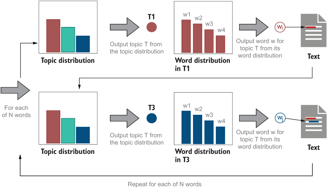
Figure 10.9 A summary of the text-generation process with LDA. For each of the N words, first a topic is selected according to the topic distribution, and then a word is selected according to the word distribution within this topic

Since the LDA algorithm does not have access to the parameters that the generative process uses, it tries to “decode” or reverse-engineer this process by learning these parameters based on the data at hand. When a new document comes along, it assumes that the document is generated by the same process with the same parameters, so it applies the parameters learned on the data, trying to answer the following question: “Given what we know about the topic and word distributions, which of the topics could have generated the given document?” It then returns the topic(s) that answer this question best.

10.2 Implementation of the topic modeling algorithm

Now that we’ve discussed the inner workings of the LDA algorithm, it’s time to apply it in practice. Figure 10.10 summarizes the processing pipeline for the algorithm.

Figure 10.10 Processing pipeline for the LDA algorithm

In this chapter, like you did in the previous one, you are going to work with the posts from the 20 Newsgroups dataset on the selected data subset. This will allow you to compare the discoveries made by your second unsupervised algorithm, LDA, in this data and see whether the assumption that the data represents the topics (i.e., labels) assigned in the original 20 Newsgroups dataset holds. Let’s remind ourselves what data we are working with and load the input data as the first step in our pipeline requires.

10.2.1 Loading the data

In the previous chapter, you learned that the popular machine-learning toolkit scikit-learn provides you not only with implementation of a variety of widely used machine-learning algorithms, but also with easy access to a number of datasets to train your skills on. The specific dataset of interest here is the famous 20 Newsgroups dataset, which is well-suited for all topic analysis-related tasks and is easily accessible via scikit-learn. (Check scikit-learn’s datasets web page for more information on the various available data: http://mng.bz/WxQl.)

As a reminder, the 20 Newsgroups dataset is a collection of around 18,000 newsgroups posts on 20 “topics”; however, not all of them have a comparable amount of data. Besides, as we’ve discussed before, exploring the results for as many as 20 topics may be quite overwhelming. To this end, in the previous chapter we restricted ourselves to a specific set of 10 topics of interest based on their diversity and the amount of data available. Table 10.1 is a reminder on the selected newsgroups labels and the amount of data you are working with.

Table 10.1 A reminder on the data from the 20 Newsgroups dataset used for topic analysis

Recall that scikit-learn’s interface to the dataset allows you to easily choose which topic labels you want to work with and which subsets of data to consider. In particular, the dataset is already split into training and test sets. Recall that when you are working with a supervised learning algorithm (e.g., the one that you used for topic classification in the previous chapter), it is important that you train the algorithm on the training data and evaluate it on the test data. Since scikit-learn already provides you with predefined subsets, it is easy to compare your results across multiple implementations, your own as well as those from the others. At the same time, such unsupervised approaches as clustering applied in the previous chapter and LDA that you are going to implement in this chapter do not make any special use of the training versus test data; in fact, they are agnostic to the particular labels that may already exist in the data and aim to identify useful groups in the data by themselves. This means that you can use the whole dataset (i.e., both training and test sets combined) to build an unsupervised model.

Listing 10.1 shows you how to access the data via scikit-learn, restricting yourself to specific topic labels from the 20 Newsgroups dataset but not to specific subsets. To start with, you import sklearn’s functionality that allows you to access the 20 Newsgroups dataset and define the load_dataset function, which takes the subset and categories list as arguments and returns the data extracted according to these restrictions. In addition, it allows you to remove extra information (e.g., headers and footers). Then you define the list of categories to extract from the data. This list contains the same categories as you’ve worked with before but note that you can always change the selection of labels to your own preferred list. When you run the load_dataset, use all as the first argument to access both training and test sets. Finally, you can access the uploaded posts applying the .data method to newsgroups_all, and, as a sanity check, print out the number of posts using len.

Listing 10.1 Code to access the Newsgroups data on specific topics

from sklearn.datasets import fetch_20newsgroups              ❶
 
def load_dataset(sset, cats):                                ❷
    if cats==[]:
        newsgroups_dset = fetch_20newsgroups(subset=sset,
                          remove=('headers', 'footers', 'quotes'),
                          shuffle=True)
    else:
        newsgroups_dset = fetch_20newsgroups(subset=sset, categories=cats,
                          remove=('headers', 'footers', 'quotes'),
                          shuffle=True)
    return newsgroups_dset
 
categories = ["comp.windows.x", "misc.forsale", "rec.autos"]
categories += ["rec.motorcycles", "rec.sport.baseball", "rec.sport.hockey"]
categories += ["sci.crypt", "sci.med", "sci.space"]
categories += ["talk.politics.mideast"]                      ❸
 
newsgroups_all = load_dataset('all', categories)             ❹
print(len(newsgroups_all.data))                              ❺

❶ Import sklearn’s functionality that allows you to access the 20 Newsgroups dataset.

❷ Define the load_dataset function to return the data extracted according to predefined restrictions.

❸ Define the list of categories to extract from the data.

❹ To access both training and test sets, use “all” as the first argument.

❺ Access the uploaded posts applying the .data method to newsgroups_all; check the number of posts using len.

The code should extract all posts on the predefined list of categories (labels), both from the training and test subsets, and as a result you should get 9,850 posts in newsgroups_all. This is what should be printed out by the code. As a reminder, there are 5,913 posts in these categories in the training set and 3,937 in the test set. You can also check these numbers against table 10.1.

10.2.2 Preprocessing the data

The data loaded so far contains whole posts, and your task is to identify topics in these posts. Since LDA works with words or tokens of similar granularity, your first task is to tokenize the posts (i.e., extract word tokens from them). Once the text is split into words, you need to consider the questions from exercise 10.2.

Listing 10.2 shows how to preprocess texts for your topic-modeling application. In particular, it uses a stemming algorithm called SnowballStemmer, which provides you with a good intermediate level of granularity. It helps the algorithm efficiency by reducing the word space to a higher extent than lemmatization, and at the same time it is less “aggressive” in merging words together than some other stemming algorithms (for comparison, you can look at the outputs of different stemmers; see www.nltk.org/howto/stem.html for some examples). This stemmer implementation is available via the NLTK toolkit, which you have extensively used before for other tasks. At the same time, listing 10.2 calls on a new toolkit, gensim, that you haven’t used before.

So far, you have gained experience using two NLP toolkits, namely NLTK and spaCy. We’ve noted before that it is good to know of the wide range of opportunities in the field, and often, when you want to develop some new application of your own, you would find that the building blocks for this application (e.g., certain preprocessing tools) are readily available. You might have also noticed that, in some respects, these toolkits have comparable functionality (e.g., both can be used to do tokenization), while in other respects they may have complementary strengths (e.g., NLTK, unlike spaCy, has access to a number of various stemmers). It is time, therefore, to add another NLP toolkit—gensim—to your tool belt (for installation instructions, see https://radimrehurek.com/gensim/).

Just like the other toolkits, gensim includes a number of useful preprocessing functions, some of which are used in listing 10.2. Specifically, you need to import SnowballStemmer from NLTK, and simple_preprocess functionality and stopwords list from gensim. SnowballStemmer supports several different languages, so you need to invoke the English version of the stemmer (other functions from NLTK and gensim are applicable to English by default). Next, you define a function stem that takes a word as an input and returns its stem as an output. Simple_preprocess functionality allows you to do several useful things at once (see detailed documentation at http://mng.bz/wo8q): it converts input text to lowercase, splits it into tokens, and returns only the tokens that are longer than min_len characters, which is set to 4 characters (inclusive) here. Finally, you iterate through the tokens, and if a token is not in the stopwords list, you apply the stemming algorithm to it and add the resulting stem to the output stored in result.

Note The “magic” number of 4 here is based on the widely recognized observation that many frequent and not topically specific words are short (i.e., about 3 characters in length). Such are, for example, common abbreviations like lol, omg, and so on. At the same time, they are unlikely to be captured by most stopwords lists.

Listing 10.2 Code to preprocess the data using NLTK and gensim

import nltk
import gensim
from nltk.stem import SnowballStemmer         ❶
from gensim.utils import simple_preprocess    ❷
from gensim.parsing.preprocessing 
import STOPWORDS as stopwords                 ❷
 
stemmer = SnowballStemmer("english")          ❸
 
def stem(text):
    return stemmer.stem(text)                 ❹
 
def preprocess(text):
    result = []
    for token in gensim.utils.simple_preprocess(
        text, min_len=4):                     ❺
        if token not in stopwords:
            result.append(stem(token))        ❻
    return result

❶ Import SnowballStemmer from nltk.

❷ From gensim, import the simple_preprocess functionality and stopwords list.

❸ Use the English version of the stemmer.

❹ Define a function stem that takes a word as an input and returns its stem as an output.

❺ The simple_preprocess functionality allows you to do several useful things at once.

❻ If a token is not in the stopwords list, apply stemming and add the stem to result.

Let’s see what effect this preprocessing step has on a specific document. The following listing applies the preprocess function to the first document from your selected newsgroups collection and prints the preprocessing result next to the original document.

Listing 10.3 Code to inspect the results of the preprocessing step

doc_sample = newsgroups_all.data[0]      ❶
print('Original document: ')
print(doc_sample)                        ❷
 
print('

Tokenized document: ')
words = []
for token in gensim.utils.tokenize(doc_sample):
    words.append(token)
print(words)                             ❸
 
print('

Preprocessed document: ')
print(preprocess(doc_sample))            ❹

❶ Extract a specific original document from the collection (e.g., the first one at index 0).

❷ Print out the original document as is.

❸ Check the output of the gensim’s tokenizer, which is produced by gensim.utils.tokenize.

❹ Check the output of the preprocess function defined in listing 10.2.

Here is what this code will produce for the first document from newsgroups_all:

Original document: 
Hi Xperts!
 
How can I move the cursor with the keyboard (i.e. cursor keys), 
if no mouse is available?
 
Any hints welcome.
 
Thanks.
 
Tokenized document: 
['Hi', 'Xperts', 'How', 'can', 'I', 'move', 'the', 'cursor', 'with', 'the', 'keyboard', 'i', 'e', 'cursor', 'keys', 'if', 'no', 'mouse', 'is', 'available', 'Any', 'hints', 'welcome', 'Thanks']
 
Preprocessed document: 
['xpert', 'cursor', 'keyboard', 'cursor', 'key', 'mous', 'avail', 'hint', 'welcom', 'thank']

You can observe the following: the original text contains over 30 word tokens, including punctuation marks. Gensim’s tokenizer splits input text by whitespaces and punctuation marks, returning individual word tokens excluding punctuation marks as a result. (Gensim’s tokenizer is part of the gensim.utils group of functions; see the description at https://radimrehurek.com/gensim/utils.html.) Finally, the preprocess function does several things at the same time: it tokenizes input text internally, converts all word tokens into lowercase, excludes not only punctuation marks but also stopwords and words shorter than 4 characters in length (thus, for example, removing “i” and “e”, which come from “i.e.”, often not covered by stopwords lists), and finally, outputs stems of the remaining word tokens. Figure 10.11 visualizes how this preprocessing step extracts the content from the original document, efficiently reducing the dimensionality of the original space.

Figure 10.11 The Preprocess function allows you to considerably reduce the dimensionality of your original feature space. It converts all words to lowercase; removes punctuation marks, stopwords, and words shorter than 4 characters; and outputs a list of stems for the remaining words.

You can also check how a particular set of documents is represented after the preprocessing steps are applied to the original texts. The following listing shows how to extract the preprocessed output from the first 10 documents in the collection.

Listing 10.4 Code to inspect the preprocessing output for a group of documents

for i in range(0, 10):                                                       ❶
    print(str(i) + "	" + ", ".join(preprocess(newsgroups_all.data[i])[:10]))❷

❶ Iterate through the documents, such as through the list of the first 10 ones.

❷ Print out each document’s index followed by the list of up to 10 first stems from this document.

The code from this listing outputs the following lists of stems for the first 10 documents in your collection:

0   xpert, cursor, keyboard, cursor, key, mous, avail, hint, welcom, thank
1   obtain, copi, open, look, widget, obtain, need, order, copi, thank
2   right, signal, strong, live, west, philadelphia, perfect, sport, fan, dream
3   canadian, thing, coach, boston, bruin, colorado, rocki, summari, post, gather
4   heck, feel, like, time, includ, cafeteria, work, half, time, headach
5   damn, right, late, climb, meet, morn, bother, right, foot, asleep
6   olympus, stylus, pocket, camera, smallest, class, includ, time, date, stamp
7   includ, follow, chmos, clock, generat, driver, processor, chmos, eras, prom
8   chang, intel, discov, xclient, xload, longer, work, bomb, messag, error
9   termin, like, power, server, run, window, manag, special, client, program

As you can see, each document is concisely summarized by a list of meaningful words. Can you tell which topic each document is on?

Now, since the LDA algorithm relies on word (or stem) occurrences to detect topics in documents, you need to make sure that the same word occurrences across documents can be easily and efficiently detected by the algorithm. For instance, if two documents contain the same words (e.g., program, server, and processor), there is a high chance they are on the same topic. The most suitable data structure to use in this case is a dictionary, where each word is mapped to a unique identifier. This way, the algorithm can detect which identifiers (words) occur in which documents and establish the similarity between documents efficiently. In fact, you have used this idea in several previous applications.

Listing 10.5 shows how to convert the full set of words occurring in the documents in your collection into a dictionary, where each word is mapped to a unique identifier, using the gensim functionality. You start by preprocessing all documents in your collection using the function preprocess, defined in listing 10.2. Then you check the length of the resulting structure. This should be equal to the number of documents you have (i.e., 9,850). After that, you extract a dictionary of terms from all processed documents, processed_docs, using gensim.corpora.Dictionary and check the size of the resulting dictionary (see the full documentation at http://mng.bz/XZX1). Finally, you check what is stored in this dictionary; for example, you can iterate through the first 10 items, printing out key (the unique identifier of a word stem) and value (the stem itself).

Listing 10.5 Code to convert word content of the documents into a dictionary

processed_docs = []
for i in range(0, len(newsgroups_all.data)):
    processed_docs.append(preprocess(
        newsgroups_all.data[i]))            ❶
 
print(len(processed_docs))                  ❷
    
dictionary = gensim.corpora.Dictionary(processed_docs)
print(len(dictionary))                      ❸
 
index = 0
for key, value in dictionary.iteritems():
    print(key, value)
    index += 1
    if index > 9:
        break                               ❹

❶ Preprocess all documents in your collection using the function preprocess defined in listing 10.2.

❷ Check the length of the resulting structure.

❸ Extract a dictionary of terms from all processed documents using gensim.corpora.Dictionary.

❹ Check what is stored in this dictionary (e.g., iterate through the first 10 items).

The code prints out the following output:

9850
39350
 
0 avail
1 cursor
2 hint
3 key
4 keyboard
5 mous
6 thank
7 welcom
8 xpert
9 copi

Figure 10.12 visualizes how the original content of the first document is converted into a succinct summary containing only the meaningful word stems after all preprocessing steps.

Figure 10.12 As a result of all preprocessing steps, the content of the original document is summarized by a selected set of meaningful word stems. As the visualization of the end result on the right shows, each selected word stem is represented with its unique identifier, and all the other words are filtered out.

Unfortunately, the dictionary that you end up with as a result of this step still contains a relatively high number of items—over 39,000—which would result in your algorithm being quite slow. Fortunately, there are more steps you can apply to reduce the dimensionality. For instance, as discussed in exercise 10.2, you can apply some cutoff thresholds, removing very frequent words and very rare ones, since none of these extremities are likely to help topic modeling. Listing 10.6 shows how to use the gensim functionality to first filter out the extremes (the words below and above certain frequency thresholds) and then convert each document into a convenient representation where the counts for each word from the dictionary are stored in tuples next to the word stem IDs. Specifically, in this code, you use dictionary.filter_extremes to discard word stems that occur in fewer than no_below=10 documents and in more than no_above=50% of the total number of documents in your collection (see documentation at http://mng.bz/XZX1). If the resulting number is over 10,000 word stems, you keep only the most frequent keep_n=10000 of them. Then you convert each document in the collection into a list of tuples, where the occurring word stem IDs are mapped to the number of their occurrences. In the end, you can check how a particular document is represented.

Listing 10.6 Code to perform further dimensionality reduction on the documents

dictionary.filter_extremes(no_below=10, no_above=0.5, keep_n=10000)
print(len(dictionary))     ❶
 
bow_corpus = [dictionary.doc2bow(doc) for doc in processed_docs]
print(bow_corpus[0])       ❷

❶ First, discard very rare and very frequent word stems; then keep only keep_n most frequent of the rest.

❷ Convert each document in the collection into a list of tuples and check the output.

The code produces the following output:

5868
 
[(0, 1), (1, 2), (2, 1), (3, 1), (4, 1), (5, 1), (6, 1), (7, 1), (8, 1)]

This means that after the “extremes”—word stems occurring in fewer than 10 and in more than 50% of the original collection of 9,850 documents—have been filtered out, you are left with 5,868 items (word stems) in the dictionary. This is a much more compact space than the original 39,350. If you print out the contents of the first document (the one that you’ve looked at in listing 10.3 and figure 10.11), you can see that the filtering step didn’t remove any of the word stems from this document, as they happen to not be within any of the “extremes.” In particular, the output like [(0, 1), (1, 2), (2, 1), . . .] tells you that the dictionary item with id=0 occurs 1 time in this document, id=1 occurs 2 times, id=2 occurs 1 time, and so on. Since after filtering the “extreme” items out the dictionary IDs returned by the code from listing 10.5 might have been overwritten (i.e., if a word stem is filtered out from the dictionary because it falls within one or another extreme, its ID is reused for the next word stem that is kept in the dictionary), it is useful to check which word stems are behind particular IDs. Listing 10.7 shows how to do that. You start by extracting a particular document from bow_corpus (e.g., the first one here). Then you print out the IDs, the corresponding word stems (extracted from dictionary), and the number of occurrences of these word stems in this document extracted from bow_corpus.

Listing 10.7 Code to check word stems behind IDs from the dictionary

bow_doc = bow_corpus[0]                ❶
 
for i in range(len(bow_doc)):
    print(f"Key {bow_doc[i][0]} ="{dictionary[bow_doc[i][0]]}":
    occurrences={bow_doc[i][1]}")      ❷

❶ Extract a particular document from bow_corpus

❷ Print out the IDs, corresponding word stems, and the number of occurrences of these word stems.

This code prints out the following output, which should be familiar to you now since you’ve already seen in figure 10.11 what word stems the first document contains:

Key 0 ="avail":       occurrences=1
Key 1 ="cursor":      occurrences=2
Key 2 ="hint":        occurrences=1
Key 3 ="key":         occurrences=1
Key 4 ="keyboard":    occurrences=1
Key 5 ="mous":        occurrences=1
Key 6 ="thank":       occurrences=1
Key 7 ="welcom":      occurrences=1
Key 8 ="xpert":       occurrences=1

Note you can inspect any document using this code. For instance, to check the content of the 100th document in your collection, all you need to do is access bow_doc = bow_corpus[99] in the first line of code in listing 10.7.

10.2.3 Applying the LDA model

Now that the data is preprocessed and converted to the right format, let’s run the LDA algorithm and detect topics in your collection of documents from the 20 Newsgroups dataset. With gensim, it is quite easy to do and running the algorithm is just a matter of setting a number of parameters. Listing 10.8 shows how to do that. You start by initializing id2word to the dictionary where each word stem is mapped to a unique ID. Then you initialize corpus to the bow_corpus that you created earlier. This data structure keeps the information on the stem occurrence and frequency across all documents in the collection. Next, you initialize lda_model to the LDA implementation from gensim (see the full documentation and description of all arguments and methods applicable to the model at https://radimrehurek.com/gensim/models/ldamodel.html). This model requires a number of arguments, which are explicitly specified in this code. Let’s go through them one by one.

First, you provide the model with corpus and id2word initialized earlier in this code. Since you have a bit of an insight into the data (specifically, you have extracted the data from 10 labeled topics), it is reasonable to ask the algorithm to find num_ topics=10. In addition, if you would like to get the same results every time you run the code, set random_state to some number (e.g., 100 here). You also need to specify how often the algorithm should update its topic distributions (e.g., after each document with update_every=1), and, for efficiency reasons, you should train it over smaller bits of data than the whole dataset (e.g., over chunks of 1,000 documents with chunksize=1000), passing through training passes=10 times. Next, with alpha='symmetric', you make sure that topics are initialized in a fair way, and with iterations=100, you put an upper bound on the total number of iterations through the data. Finally, per_word_topics ensures that you learn word-per-topic as well as topic-per-document distributions. In the end, you print out the results: use -1 as an argument to print_topics to output all topics in the data, and for each of them, print out its index and the most informative words identified for the topic.

Listing 10.8 Code to run the LDA algorithm on your documents

id2word = dictionary                                             ❶
corpus = bow_corpus                                              ❷
 
lda_model = gensim.models.ldamodel.LdaModel(corpus=corpus,
                                           id2word=id2word,      ❸
                                           num_topics=10,
                                           random_state=100,     ❹
                                           update_every=1,
                                           chunksize=1000,
                                           passes=10,            ❺
                                           alpha='symmetric',
                                           iterations=100,
                                           per_word_topics=True) ❻
 
for index, topic in lda_model.print_topics(-1):
    print(f"Topic: {index} 
Words: {topic}")                    ❼

❶ Initialize id2word to the dictionary where each word stem is mapped to a unique ID.

❷ Initialize corpus to the bow_corpus that you created earlier.

❸ Initialize lda_model to the LDA implementation from gensim.

❹ It is reasonable to ask the algorithm to find num_topics=10.

❺ Specify how often the algorithm should update its topic distributions and train it over smaller bits of data.

❻ Set up the remaining parameters.

❼ Output all topics and for each of them print out its index and the most informative words identified.

The code produces the following output:

Topic: 0 
Words: 0.021*"encrypt" + 0.018*"secur" + 0.018*"chip" + 0.016*"govern" + 0.013*"clipper" + 0.012*"public" + 0.010*"privaci" + 0.010*"key" + 0.010*"phone" + 0.009*"algorithm"
Topic: 1 
Words: 0.017*"appear" + 0.014*"copi" + 0.013*"cover" + 0.013*"star" + 0.013*"book" + 0.011*"penalti" + 0.010*"black" + 0.009*"comic" + 0.008*"blue" + 0.008*"green"
Topic: 2 
Words: 0.031*"window" + 0.015*"server" + 0.012*"program" + 0.012*"file" + 0.012*"applic" + 0.012*"display" + 0.011*"widget" + 0.010*"version" + 0.010*"motif" + 0.010*"support"
Topic: 3 
Words: 0.015*"space" + 0.007*"launch" + 0.007*"year" + 0.007*"medic" + 0.006*"patient" + 0.006*"orbit" + 0.006*"research" + 0.006*"diseas" + 0.005*"develop" + 0.005*"nasa"
Topic: 4 
Words: 0.018*"armenian" + 0.011*"peopl" + 0.008*"kill" + 0.008*"said" + 0.007*"turkish" + 0.006*"muslim" + 0.006*"jew" + 0.006*"govern" + 0.005*"state" + 0.005*"greek"
Topic: 5 
Words: 0.024*"price" + 0.021*"sale" + 0.020*"offer" + 0.017*"drive" + 0.017*"sell" + 0.016*"includ" + 0.013*"ship" + 0.013*"interest" + 0.011*"ask" + 0.010*"condit"
Topic: 6 
Words: 0.018*"mail" + 0.016*"list" + 0.015*"file" + 0.015*"inform" + 0.013*"send" + 0.012*"post" + 0.012*"avail" + 0.010*"request" + 0.010*"program" + 0.009*"includ"
Topic: 7 
Words: 0.019*"like" + 0.016*"know" + 0.011*"time" + 0.011*"look" + 0.010*"think" + 0.008*"want" + 0.008*"thing" + 0.008*"good" + 0.007*"go" + 0.007*"bike"
Topic: 8 
Words: 0.033*"game" + 0.022*"team" + 0.017*"play" + 0.015*"year" + 0.013*"player" + 0.011*"season" + 0.008*"hockey" + 0.008*"score" + 0.007*"leagu" + 0.007*"goal"
Topic: 9 
Words: 0.013*"peopl" + 0.012*"think" + 0.011*"like" + 0.009*"time" + 0.009*"right" + 0.009*"israel" + 0.009*"know" + 0.006*"reason" + 0.006*"point" + 0.006*"thing"

Figure 10.13 visualizes this output for the first topics, listing the top 3 most highly weighted words in each for brevity.

Figure 10.13 The output from listing 10.8. For brevity, only the first 6 topics with their top 3 most informative words are included.

In this output, each topic with its unique ID (since you are using an unsupervised approach, this algorithm cannot assign the labels, so it returns IDs) is mapped with a set of most informative words that help the algorithm associate documents with this specific topic. For instance, the first topic Topic 0 is characterized by such word stems as encrypt (for encryption, encrypted, etc.), secur (for secure, security, etc.) and chip; the third topic Topic 2 can be identified by the word stems like window (as in Windows), server, program, and so on. Note that the numerical values included in front of the word stems show the relative weight of each word in the topic (or its probability score), and the + sign suggests that the topic is composed of all these words in the specified proportion. Now let’s attempt exercise 10.4.

Let’s discuss this exercise together. To begin with, this exercise should remind you of exercise 9.7, where you tried to interpret the clusters as topics based on the most informative words within each identified cluster. Let’s use a copy of table 9.6 here (table 10.2) to interpret the topics identified by LDA and map them to the clusters from chapter 9 on the one hand and to the labels from the 20 Newsgroups dataset on the other.

Table 10.2 Possible topic labels for the identified topics

As you can see from the interpretation of the output, just like with another unsupervised approach, clustering, implemented in the last chapter, the LDA algorithm comes up with a topic allocation that does not necessarily coincide with the topic labels from the original dataset. Some original topics (e.g., rec.sport.baseball and rec.sport.hockey), appear to be merged into one topic, Topic 8. At the same time, such topics as talk.politics.mideast and misc.forsale are split into multiple groups. Note that you’ve got a similar result from the clustering algorithm, which also split these topics into two clusters each. This shows that there might truly be quite diverse subtopics discussed under both titles, and they perhaps shouldn’t be thought of as single homogeneous topics. However, there is something new that is discovered by the LDA algorithm in the data, which was not observed in the clustering output. First, it seems like sci.med and sci.space correspond to a single topic, Topic 3. Since both topics are science-related (note that they both come from the sci. thread), the algorithm identifies their internal similarities. Second, the LDA algorithm identifies Topic 1, characterized by such word stems as copi (as in copies), book, and comic. This is a novel discovery in the data, encompassing documents that potentially cover a yet unidentified topic related to books. Figure 10.14 summarizes the topics discovered by LDA and maps them, where possible, to the labels from the 20 Newsgroups data.

Figure 10.14 Summary of the topics discovered by the LDA algorithm with the labels from the 20 Newsgroups dataset assigned to the identified topics, where possible

10.2.4 Exploring the results

Given that you are working with an unsupervised algorithm, it may be hard to interpret the results in a precise, quantitative way. In this section, you’ll be looking into several approaches to results exploration.

We’ve said earlier in this chapter that the LDA algorithm interprets each document as a mixture of topics. It is, in fact, possible to measure the contribution of the topics and, in particular, identify the main contributing topic for each document together with its most informative words. Listing 10.9 does exactly that. In this code, you first define the function analyse_topics, which takes as input the LDA model, the word-frequency-per-document structure from the corpus, and the original collection of texts. This function returns as output the main topic for each document (stored in main_topic), contribution of this topic to the mixture of topics in the document (stored in percentage), the most informative words (stored in keywords), and the original word stems from the document (in text_snippets). Then, for each document in the collection (corpus), you extract the most probable topic mixture identified by LDA as topic_list[0], sort the topics from the most probable to the least probable using sorted(..., reverse=True) applied to the topic probability score stored in field x[1], and extract the most probable topic from the resulting interpretation (see https://docs.python.org/3/howto/sorting.html on sorting with a lambda expression). It can be identified as the first item in the sorted list (thus, the identifier j=0), and it corresponds to a tuple (topic id, topic proportion). Next, you extract topic keywords using the show_topic functionality (check documentation at https://radimrehurek.com/gensim/models/ldamodel.html) and store the main topic ID (topic_num), topic contribution as percentage rounded up to 4 digits after the decimal point (prop_topic), the first 5 most informative topic keywords (topic_keywords), and a list of up to 8 word stems from the original text (the limit of 8 is chosen for readability purposes only). Finally, you apply the analyse_topic function to the dataset and store the results.

Listing 10.9 Code to identify the main topic for each document in the collection

def analyse_topics(ldamodel, corpus, texts):                      ❶
    main_topic = {}
    percentage = {}
    keywords = {}
    text_snippets = {}                                            ❷
    
    for i, topic_list in enumerate(ldamodel[corpus]):
        topic = topic_list[0]            
        topic = sorted(topic, key=lambda x: (
                       x[1]), reverse=True)                       ❸
 
        for j, (topic_num, prop_topic) in enumerate(topic):
            if j == 0:                                            ❹
                wp = ldamodel.show_topic(topic_num)               ❺
                topic_keywords = ", ".join([word for word, prop in wp[:5]])
                main_topic[i] = int(topic_num)
                percentage[i] = round(prop_topic,4)
                keywords[i] = topic_keywords
                text_snippets[i] = texts[i][:8]                   ❻
            else:
                break
    return main_topic, percentage, keywords, text_snippets
 
main_topic, percentage, keywords, text_snippets = analyse_topics(
    lda_model, bow_corpus, processed_docs)                        ❼

❶ analyse_topics takes as input the LDA model, corpus, and the original collection of texts.

❷ Return the main topic, its contribution, the most informative words, and the original word stems.

❸ For each document in the collection, extract the most probable topic mixture and sort the topics.

❹ Extract the most probable topic from the resulting interpretation.

❺ Extract topic keywords using the show_topic functionality.

❻ Store the main topic ID, its contribution, the most informative topic keywords, and a list of word stems.

❼ Apply the analyse_topic function to the dataset and store the results.

Next, listing 10.10 shows how to print out the results for a specified range of documents using a convenient tabulated format.

Listing 10.10 Code to print out the main topic for each document in the collection

indexes = []
rows = []
for i in range(0, 10):                              ❶
    indexes.append(i)
rows.append(['ID', 'Main Topic', 'Contribution (%)', 'Keywords', 'Snippet'])
 
for idx in indexes:
    rows.append([str(idx), f"{main_topic.get(idx)}", 
                f"{percentage.get(idx):.4f}",
                f"{keywords.get(idx)}
",
                f"{text_snippets.get(idx)}"])
 
columns = zip(*rows)
column_widths = [max(len(item) for item in col) for col in columns]
for row in rows:
    print(''.join(' {:{width}} '.format(row[i], width=column_widths[i]) 
                  for i in range(0, len(row))))     ❷

❶ Extract the output for the first 10 documents for simplicity.

❷ Use the familiar printout routine to print the results in a tabulated manner.

The code returns the output shown in table 10.3 for the first 10 documents in the collection ([...] is used to truncate the output for space reasons, and a table is used to make the output more readable). Note that you can always print the output for any specified number of documents, as well as return more than 5 most informative keywords per topic and more than 8 word stems from each document—just change these settings in listing 10.9.

Table 10.3 Output printed out by the code from listing 10.10

As this output suggests, both the first and the tenth documents are on Topic 2, characterized by such keywords as server, program, and file (you can also see from the text snippets why these documents may be topically related). At the same time, document 3 is on a topic related to sports, as is exemplified by such keywords as game, team, and play.

Finally, we’ve started this chapter with the discussion on the LDA model saying that this is a unique model that allows you to investigate the interplay between words and topics in the documents. So far, your analysis of the results didn’t allow you to appreciate the full extent of the model predictions. Luckily, there are a number of helpful visualization tools developed around this model, one of which is particularly useful for the analysis—pyLDAvis (available at https://github.com/bmabey/pyLDAvis). Install it following the instructions prior to running the code from listing 10.11. This tool provides you with an interactive interface to the LDA output, where you can explore both the topic distribution per documents in your collection and word distribution per topic, which is very useful when you try to interpret the output of the LDA model. You can run this tool and visualize the results directly in the Jupyter Notebook, or you can save the results in an external HTML file.

Listing 10.11 introduces the use of this tool in a concise piece of code. You start by importing pyLDAvis functionality (for newer versions of the tools, use import pyLDAvis.gensim_models) and making sure that the results can be visualized within the notebook. To apply the visualization tool, you’ll need to pass in the LDA model, the data with the word occurrences in corpus, and the mapping between word stems and their IDs from id2word as arguments (for newer versions of the tools, use pyLDAvis.gensim_models.prepare(...)). Finally, you can run the visualization and inspect the results in the notebook.

Listing 10.11 Code to visualize the output of LDA using pyLDAvis

import pyLDAvis.gensim                          ❶
pyLDAvis.enable_notebook()                      ❷
vis = pyLDAvis.gensim.prepare(lda_model, corpus, dictionary=lda_model.id2word)              ❸
vis                                             ❹

❶ Import pyLDAvis functionality.

❷ Make sure the results can be visualized in the notebook.

❸ Pass in the LDA model, the data with the word occurrences, and the mapping between word stems and their IDs.

❹ Run the visualization.

This code produces an interactive visualization of the words and topics, which you can directly explore in your notebook. The topics are represented as bubbles of the size relative to their distribution in the data (in addition, bubbles representing similar topics are located closer to each other in the space on the left), and the word stem list on the right shows contribution of each stem to each topic. You can hover your mouse over both the topics on the left, exploring word contribution to the topic, and over the words on the right, exploring word membership within various topics.

For instance, figure 10.15 visualizes word composition for a specific topic, denoted as Topic 9, which can be interpreted as a sales topic. It contains words like price, sale, offer, and so on. At the same time, the chart on the right makes it clear that sale contributes to this topic fully, while price is almost fully associated with this topic, and words like good and work contribute to this topic only partially, since they probably are widely used elsewhere.

Figure 10.15 Topic 9, visualized with a bubble on the left, is composed of all the words that are highlighted in the list on the right. From these words’ composition, you can tell that Topic 9 here corresponds to sales. The words are ordered by their relative contribution to the topic (e.g., price and sale are the main contributors, and most of their use corresponds to the documents on sales). At the same time, good contributes to this topic, but, as the chart shows, it is also used elsewhere.

How can you check where the rest of the word “weight” goes? If you hover over the words in the chart on the right, it will show you the topic membership for the words, highlighting the relevant topic bubbles. For instance, figure 10.16 shows that the word game (highlighted in bold) is associated with two topics—one related to sales and another to sports. Finally, if you’d like to explore other visualization techniques for topic modeling, the following post may provide you with further ideas: http://mng.bz/qYgw.

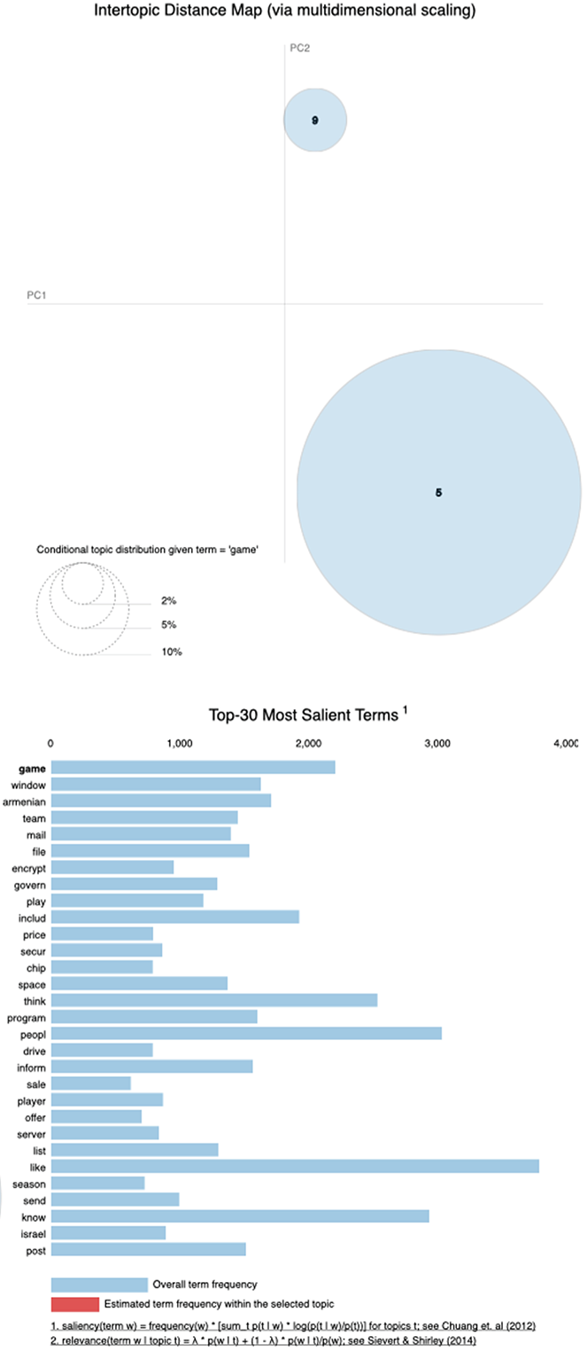
Figure 10.16 The word game is associated with two topics. When you hover over it on the right, two topic bubbles are highlighted on the left—Topic 9 associated with anything sales-related, and Topic 5 associated with sports. The relative size of the bubbles tells you that game is much more strongly associated with the sports in Topic 5.

Summary

• Topic analysis as addressed within the unsupervised paradigm allows the applied algorithm to explore the data and identify interesting correspondences without any regard to predefined labels.

• Latent Dirichlet allocation (LDA) is a widely used unsupervised approach for topic modeling. This approach treats each document as a mixture of topics and allows you to explore both document composition in terms of topics and topic composition in terms of words. If you’d like to learn more about this insightful algorithm, check David Blei’s home page at http://www.cs.columbia.edu/~blei/ topicmodeling.html, and take a look at his paper on Probabilistic Topic Models here: http://www.cs.columbia.edu/~blei/papers/Blei2012.pdf.

• LDA is a generative model. It assumes that each document is generated by an abstract generative process, which first selects an appropriate topic according to topic distribution and then picks words from this topic according to the word distribution per topic.

• The topic structure, including the topics themselves, their distributions in documents, and word-to-topic assignments, is a latent (i.e., hidden) structure, thus the name of the algorithm. It is estimated and adjusted on the basis of the only observed parameter—words in documents.

• Word distribution and topic distribution are the two fundamental blocks in the algorithm. The algorithm tries to estimate them directly from the data.

• Gensim is another useful NLP toolkit. It is particularly suitable for all tasks around word meaning and topic modeling.

• Using gensim, you can not only preprocess textual data but also apply an LDA model. As a result, this algorithm may help you discover new topics in the data.

• As is common with unsupervised approaches, the results may be hard to evaluate quantitatively. pyLDAvis is an interactive visualization toolkit for topic modeling interpretation, which allows you to explore topic composition in terms of words and word membership in terms of topics.

Solutions to miscellaneous exercises

Exercise 10.2

You have done feature selection and come across dimensionality reduction in a number of previous applications. Often, this process relies on your intuition or observations on the task and the data. Alternatively, you can run some preliminary experiments to figure out what the best settings for a specific algorithm would be. The following are reasonable choices for this scenario:

1. The choice you are given is between considering each word form (e.g., car and cars, welcome and welcoming) as a separate feature or converting every word form to its dictionary version (i.e., lemma), which will merge car and cars into a single representation car, or extracting the core of each word form (stem), thus merging some words and lemmas even further. For instance, this will result in both welcome and welcoming to be represented as welcom. (This is a reminder of the differences between lemmas and lemmatization and between stems and stemming, discussed in chapter 3.) This means that the solution that results in the larger number of features is the one that relies on full word forms; however, there is often no topic-related difference between car and cars or sell and sells. In practice, for algorithms that quickly increase in complexity with the number of features, it is better to consider lemmatization or stemming. Stemming produces a more condensed feature space as compared to lemmatization; thus it would make the algorithm more efficient. The downside may be that, depending on the data, it might occasionally merge topically different words into a single representation.

2. You may consider any or all of the following strategies:

   • Remove stopwords since they usually do not bear any topic-related meaning (e.g., not, of, a).

   • Remove any other words that are likely to not bear any topic-related meaning even if they are not covered by a particular stopwords list. Often such words are short ones (e.g., various abbreviations like lol or omg).

   • Remove extremely rare words, as they might not occur in any further documents.

   • Remove very frequent words. Just like stopwords, they are unlikely to distinguish between topics (e.g., post, which might be used in a wide range of posts in the newsgroups data).

Exercise 10.3

The first line simply tells you that all 9,850 documents from the original collection have been successfully preprocessed and stored in the processed_docs list. The number of word stems in the dictionary is printed next; it equals 39,350. Finally, you can see a list of the first 10 word stems from the created dictionary, where each identifier is mapped uniquely to a stem. For instance, the first document that you looked into in listing 10.3 and that was analyzed in figure 10.11 consists of the stems ['xpert', 'cursor', 'keyboard', 'cursor', 'key', 'mous', 'avail', 'hint', 'welcom', 'thank']. Note that there are 10 stems altogether; however, cursor occurs in this list twice. When gensim converts the lists of words from each document into a single dictionary, it does two things: (1) each word can map to only a single identifier, so that multiple occurrences of the same word are mapped to the same identifier, and (2) the words are ordered alphabetically. If you wanted to manually convert ['xpert', 'cursor', 'keyboard', 'cursor', 'key', 'mous', 'avail', 'hint', 'welcom', 'thank'] into a dictionary of terms using this strategy, you would first sort the words alphabetically as in ['avail', 'cursor', 'cursor', 'hint', 'key', 'keyboard', 'mous', 'thank', 'welcom', 'xpert']; then you would remove duplicates; and finally, you would assign unique identifiers to each word stem as in [0='avail', 1='cursor', 2='hint', 3='key', 4='keyboard', 5='mous', 6='thank', 7='welcom', 8='xpert']. This is precisely the output that you are getting from listing 10.5. Once the algorithm is finished with document 1, it moves on to the next document, applies the same procedure, and appends the other unique words to the dictionary. For instance, you see that key 9 corresponds to the word stem copi, which comes from the second document (you can see this word stem in the output from listing 10.4).