5 Author profiling as a machine-learning task
- Implementing your user profiling algorithm
- Exploring NLP techniques with NLTK and spaCy
- Introducing scikit-learn
- Applying Decision Trees machine-learning classifier
In this and the next chapter, you will build your own algorithm that can identify the profile or even the precise identity of an anonymous author of a text based solely on their writing. As you will find out over the next two chapters, this task brings together several useful NLP concepts and techniques that were introduced in the previous chapters. You’ve learned that
-
Tokenizers can be applied to split text into individual words.
-
Words may be meaningful, or they may simply express some function (e.g., linking other, meaningful words together). In this case, they are called stopwords, and for certain NLP applications you will need to remove them.
-
Words are further classified into nouns, verbs, adjectives, and so on, depending on their function. Each of such classes is assigned a part-of-speech tag, which can be identified automatically with a POS tagger.
-
Words of different functions play different roles in a sentence, and these roles and relations between words with different functions can be identified with a dependency parser.
-
Words are formed of lemmas and stems, and you can use lemmatizers and stemmers to detect those.
You have also learned how to use two NLP toolkits to perform these processing steps: NLTK was introduced in chapter 2 and spaCy in chapter 4. This chapter will further exemplify the routines with each of these toolkits and will show how to combine the two.
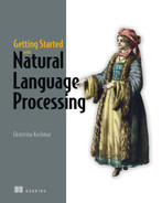
Chapter 2 also presented you with an example of an NLP task, spam filtering, that is traditionally addressed using machine-learning approaches. Figure 5.1 shows the machine-learning process from chapter 2.
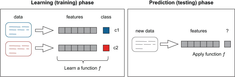
Figure 5.1 Text classification using a machine-learning approach
In spam detection, texts are coming from two different sources called classes—spam and ham (not spam). Each of these classes can be characterized with a distinctive use of words that helps users tell whether an incoming email is spam or ham, should they happen to read it. In a similar fashion, machines can be taught to distinguish between the two classes based on the words used in spam messages and filter out “bad” emails before they reach the user, thus saving the user precious time and effort.
Machine learning provides you with a whole set of powerful algorithms that can learn from data how to distinguish between classes or how to make predictions; therefore, such algorithms are widely used in NLP. As soon as the task at hand can be presented as a clear set of classes, which can each be characterized with a set of distinguishable properties, you can apply a machine-learning classifier to automatically assign instances to the relevant classes. The set of distinguishable characteristics that uniquely describe each of the classes are called features in the machine-learning context, and the process of selecting which type of information represents such useful distinguishable characteristics is called feature engineering.
This chapter will show you how to perform feature engineering for an NLP task. It will specifically focus on building a machine-learning (ML) pipeline, following all the steps from data preparation to results evaluation. Chapter 2 relied on the use of a specific ML classifier, Naïve Bayes. Since Naïve Bayes is widely used in practice, many toolkits, including NLTK, have an implementation of this algorithm ready for your use. However, even though NLTK provides you with implementation of some machine-learning algorithms, it is primarily an NLP toolkit. Therefore, in this and the next chapters you will learn how to use an ML toolkit, scikit-learn, which will provide you with a useful set of resources and techniques to apply in an ML project.
As we said, many NLP tasks can be represented as ML tasks. You need three components in place:
-
You should be able to define the task in terms of distinguishable classes (e.g., spam versus ham).
-
You should be able to tell the machine which types of information are good to use as features (e.g., words in an email are often predictive of its class).
-
You should have some labeled data at hand. For example, you may have some previously received normal as well as spam emails, or there may exist some open-source dataset like Enron that we used in chapter 2.
This setup works well for supervised machine-learning algorithms, where we know what the classes are and can provide the machine with the data to learn about these classes. In this chapter, we will address a task that is well suited for both practicing your NLP skills and learning how to build an ML project—user or author profiling. This task helps you identify the profile of an author of a text based solely on their writing. Such a profile may cover any range of characteristics, including age, level of education, and gender, and in some cases may even help you detect the precise identity of an anonymous writer.
5.1 Understanding the task
Let’s start with a scenario. Imagine that you have received an anonymous message, and you are certain that the anonymous sender is actually someone from your contacts list, with whom you have previously exchanged correspondence. Using NLP and ML techniques and NLTK and spaCy libraries that you’ve learned about in the previous chapters, build an algorithm that will help you identify who from your contacts list is the anonymous author, based solely on this piece of writing. To help you with this task, you can use all the previous messages you ever received from any of your contacts. If this algorithm cannot identify the author uniquely, can it at least help you narrow down the set of “suspects”?
It turns out that, if you have a set of texts written previously by each of your contacts, you can train a machine-learning algorithm to detect which of the potential authors the particular piece of writing belongs to. Impressive as it may seem, it relies on the idea that each of us has a distinctive writing style. For example, have you ever noticed that you tend to use however rather than but (like I do)? Or perhaps you use expressions like well, sort of, or you know a lot? Have you, perhaps, noticed that you normally use longer and more elaborate sentences than most of your friends? All of these are peculiar characteristics that can tell a lot about the author and may even give away the author’s identity. Such writing habits are also behind personalization strategies. For instance, you might notice that a predictive keyboard on your smartphone adapts to your choice of words and increasingly suggests words and phrases that you would prefer to use anyway. Now let’s look more closely into two use cases for the task of user/ author profiling.
5.1.1 Case 1: Authorship attribution
Perhaps one of the most famous cases for authorship attribution is that of the Federalist Papers, which are a collection of 85 articles and essays written by Alexander Hamilton, James Madison, and John Jay in 1787-1788 under the pseudonym “Publius” to promote the ratification of the U.S. Constitution (https://en.wikipedia.org/wiki/The_Federalist_Papers). It is hard to underestimate the importance of these articles for America’s history, yet at the time of publication, the authors of these articles preferred to hide their identities. The work of the American historian Douglass Adair in 1944 provided some of the most widely accepted assignments of authorship in this collection, and it has been corroborated in 1964 by computational analysis of word choice and writing style. However, authorship of as many as 12 out of 85 essays in this collection is still disputed by some scholars, which shows that this is by no means an easy task!
Another famous example of authorship attribution studies is the contested authorship of the works by William Shakespeare (http://mng.bz/lx8j). For some time, a theory has been circulating suggesting that the works authored under the name of Shakespeare cover topics and use a writing style that are incompatible with the social status and the level of education that the claimed author, William Shakespeare from Stratford-upon-Avon, possessed. The alternative authorship suggestions included “Shakespeare” being a pseudonym used by some other poet or even a whole group of authors at the time, with William Shakespeare himself simply acting as the cover for this true author or authors. Here, again, computational analysis has been used to prove that the writing style and the word choice in the works authored by William Shakespeare are actually consistent with his identity.
These examples provide you with the historical perspective for the task, but they don’t tell you much about the modern application of this task. How is authorship attribution used these days? For a start, it has applications in security and forensics, where there is often a need to detect whether a particular individual is the author of a particular piece of writing, or whether a particular individual is who they claim they are, based on their writing. Another area in which authorship attribution is of help is fake news—a problem that has recently attracted much attention and that is concerned with an attempt of some individuals to spread misinformation, often in order to sway public opinion. As you may expect, authorship attribution is particularly challenging on the web, where the identity of the users can be easily hidden, so this is where computational methods of detecting the potential authors or detecting whether a set of posts are produced by the same author are of most help.
5.1.2 Case 2: User profiling
We all have our particular writing styles and our preferred words that we tend to use more often than other people around us. What explains such phenomena? A lot of it comes from our background: our upbringing, education, profession, and environment have a significant effect on how we speak and write. In addition, words come in and out of fashion, so our word choice can also give away our age. Figure 5.2 shows how the usage of the words awesome, cool, and tremendous changed over time across a range of books available through Google Books. Note how around 1940 both tremendous and cool were used with approximately equal frequency, but after then the use of tremendous has been declining, while that of cool has been on the rise since 1970s, which can be partially explained by it acquiring a new meaning similar to tremendous and awesome themselves.
Note You can explore changes in the word usage with the interactive Google Books Ngram Viewer interface: https://books.google.com/ngrams/. For more information on how to use the interface, check https://books.google.com/ngrams/info.

Figure 5.2 Change in word frequencies between years 1800 and 2000 according to Google Books
Recent research shows that a number of characteristics, including age, gender, profession, social status, and similar traits can be predicted from the way one tweets. How can this be of further use? Apart from the word choice, people of different social groups have different preferences along various dimensions. Suppose you are providing a particular service or product to a wide and diverse set of users. You don’t collect any personal information about them, but you have access to some of their writing (e.g., a set of reviews about your product or a forum where they discuss their experience). Naturally, they may have different opinions about the product or service based on their personal characteristics. But equipped with an algorithm that can distinguish between groups of users of different age, gender, social status, and so on based on their writing, you can further adapt the product or service you provide to the needs of each of these groups.
Note There are multiple publications around these topics. Examples include Preotiuc-Pietro et al. (2015), “Studying User Income Through Language, Behaviour, and Affect in Social Media” (http://mng.bz/BMX8); Preotiuc-Pietro et al. (2015), “An analysis of the User Occupational Class through Twitter Content (www.aclweb.org/anthology/P15-1169.pdf); and Flekova et al. (2016), “Exploring Stylistic Variation with Age and Income on Twitter” (www.aclweb.org/anthology/P16-2051.pdf), among others.
Now, how should you approach this task computationally? We have said in the beginning of this chapter that user profiling is a good example of an ML task, so let’s define the components: the classes, the features, and the data.
Figure 5.3 illustrates the two cases of authorship attribution and user profiling.

Figure 5.3 In the authorship attribution case, each author represents a separate class; in the user profiling case, each group of users (e.g., female authors and male authors) forms a separate class.
Finally, you need data. In this case, data refers to a collection of texts that are appropriately labeled with the names of the authors who produced them for authorship attribution, or with the groups of users for user profiling. Then you can apply an ML classifier of your choice and make it learn to distinguish between different authors or groups of authors based on their writing and types of characteristics that you identified for the algorithm as features.
It’s now time to define a mental model for the ML pipeline that you are going to build in this chapter. Figure 5.4 presents the mental model.
We have discussed the first three steps of the pipeline so far. You know how to define the classes and the features and know what the data should contain. This chapter will focus on more informed feature engineering for the task of authorship attribution. In addition, the last two steps in figure 5.4 suggest that once you have extracted features and applied an ML algorithm, you may get back to the feature extraction step and expand the feature set with new types of features. You can also do so and redefine the feature set as well as the ML classifier once you have evaluated the results.
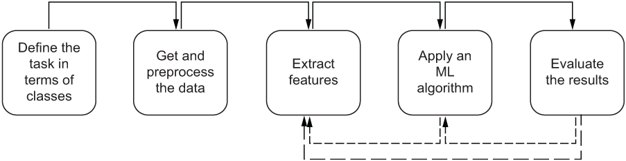
Figure 5.4 Mental model for a supervised machine-learning classification task
So far, you have looked into one particular example of an ML algorithm applied to an NLP task—Naïve Bayes using NLTK implementation. In this chapter, we will explore in more detail what other classifiers are available for your use, how to apply them to language-related data, and crucially, how to evaluate whether a classifier of your choice with a specific set of features is doing a good job.
5.2 Machine-learning pipeline at first glance
Let’s now go through the steps in this pipeline one by one. We will start with the question of what represents a good dataset for this task, and then we will proceed with building a benchmark machine learning model—something that is relatively straightforward and easy to put together. This benchmark model will set up an important point of comparison for you. Any further model with a different set of features or a different algorithm will have to beat the results of the benchmark model; otherwise, you will know that the task can be easily solved with the algorithm that you’ve tried first. Finally, we will explore the results and see how the pipeline can be improved to achieve increasingly better results.
5.2.1 Original data
In any machine-learning task, data plays a crucial part. Whatever algorithm you are using, the quality of the data decides whether the algorithm will be able to learn how to solve the task. That is, if the data is of poor quality or does not fairly represent the task at hand, it is hard to expect any machine-learning algorithm of any level of sophistication to be able to learn reliably from such data. This is not surprising, if you consider the following: the best learning algorithm known is the human brain, yet even the human brain can get confused if it is provided with conflicting and contradicting evidence. So, for both human learning and machine learning, it is important to define the task from the start and to provide some illustrative examples for the instances of different classes.
Whether you are working on the authorship attribution or on the user profiling variety of the task, good data is not easy to come by. Ideally, you want a set of texts written by different authors or separate sets of authors reliably identified as such. Let’s start with a simpler case. Let’s use a collection of literary works produced by well-known authors to address the authorship attribution task. There are two clear benefits to that: First, such an experiment does not violate any privacy rights of any users, as famous writers have clearly claimed their authorship on these pieces of writing. Second, texts by famous authors are abundant in quantity, so we can reliably find enough data representing each author (i.e., each class). Exercise 5.3 provides you with an example of the task we will try to solve in this chapter.

Figure 5.5 Who wrote these lines?
The point of this exercise is not to test your knowledge of literary works. It is rather to illustrate a number of points about the task of authorship attribution. First, the word choice and spelling can help you a lot. In this example, Early Modern English (http://mng.bz/BMBv) spelling suggests that a piece comes from a play by Shakespeare; if there happened to be an excerpt with words spelled in an American spelling tradition (e.g., favorite versus favourite, publicize versus publicise), you could have attributed such an excerpt to Ernest Hemingway as the only American writer on the list. Second, you may have noticed that apart from spelling, there are no other obvious clues that could suggest that pieces one and three come from the same author, as do pieces two and four. This is what makes this task challenging, and in what follows you will find out whether words are the only reliable characteristic features that can identify the author.
In this chapter, we will start with a simpler case of two authors, making it a binary classification task. First of all, we will look into how to get the data and extract the relevant information from it. For that, we will once again turn to NLTK. One of the useful features of this toolkit is that it provides you with access to a wide range of language resources and datasets. For instance, it contains several literary works that are available in the Project Gutenberg collection (www.gutenberg.org). Listing 5.1 shows how you can access these texts.
Note In addition to the NLTK toolkit, you need to install NLTK data as explained at www.nltk.org/data.html. Running nltk.download() will install all the data needed for text processing in one go. In addition, individual tools can be installed separately (e.g., nltk.download('gutenberg') installs the texts from Project Gutenberg available via NLTK).
Listing 5.1 Code to extract literary works from Project Gutenberg via NLTK
import nltk
nltk.download('gutenberg')           ❶
from nltk.corpus import gutenberg    ❷

gutenberg.fileids()                  ❸
❶ Download NLTK’s Gutenberg collection.
❷ Import data from the Gutenberg collection.
❸ Print out the names of the files.
The code will print out a list of 18 files that contain literary works by 12 authors. In particular, the list contains the following pieces:
['austen-emma.txt',
'austen-persuasion.txt',
'austen-sense.txt',
'bible-kjv.txt',
...
'shakespeare-caesar.txt',
'shakespeare-hamlet.txt',
'shakespeare-macbeth.txt',
'whitman-leaves.txt']
For instance, the first three entries correspond to Jane Austen’s Emma, Persuasion, and Sense and Sensibility. Despite the fact that NLTK’s interface to Project Gutenberg gives you access to only a handful of texts, this is enough for our purposes in this chapter. Let’s select two authors that we will use for classification. Jane Austen and William Shakespeare are a natural choice, since three pieces of writing are included in this collection for each of them, which means that we’ll have enough data to work with. Our task will be akin to that in exercise 5.3: we will build an algorithm that can attribute a given sentence to Author1="Jane Austen" or Author2="William Shakespeare". As you have learned from exercise 5.3, there might be some helpful clues in the writing, such as particular words or characteristic spelling; however, the task is not always straightforward, so let’s see how successfully an ML algorithm can deal with it. In general, the main reason we are working with these two authors in this chapter is the availability of the data and, perhaps, in real life we won’t be trying to distinguish between this particular pair of authors. However, the techniques overviewed in this and the next chapter are applicable to the task of authorship identification in general and you can easily transfer them to any of your own real-life projects.
Although NLTK’s interface gives you access to the full texts of Emma, Macbeth, etc., it is sentences that we will try to attribute to authors in this chapter. Why is this more useful in practice? The length of the full text varies a lot across literary works, but it will most typically be a matter of hundreds of thousands or even millions of words and thousands of sentences. It is much longer than what you might want to classify in practice: a typical message that you might try to classify will not run to the length of any of the literary works, so it is more useful to explore which approaches will work at a sentence level. This also makes your task more challenging. A sentence outside of its context might be harder to attribute than a whole body of Macbeth. Conveniently, NLTK actually allows you to directly access the set of sentences from each of these works, so you don’t need to split them into sentences yourself. For that, just use gutenberg.sents(name_of_file).
Now comes the point at which you need to let the algorithm know which data it may use to learn from. You may recall from chapter 2 that the bit of data that is used by the algorithm to learn from is called training set, and the bit that is used to evaluate the results (i.e., test how well the algorithm can do the task) is called test set. Typically, you would want to provide the algorithm with more data for training, so let’s use two out of three works by each of the authors to train the classifier, and the third work to test it. Listing 5.2 shows how to define the training and test sets for the two authors. In this code, you define training sets for the two authors by combining the sentences from two out of three works available for each of them. The test sets then contain the sentences from the third work by each author. You can inspect the data in both sets by printing out some of the uploaded sentences and the length of the sentence lists in the sets.
Listing 5.2 Code to define training and test sets
nltk.download('punkt')                                ❶

author1_train = gutenberg.sents('austen-emma.txt') + gutenberg.sents('austen-persuasion.txt')         ❷
print (author1_train)                                 ❸
print (len(author1_train))                            ❹

author1_test = gutenberg.sents('austen-sense.txt')
print (author1_test)
print (len(author1_test))                             ❺

author2_train = gutenberg.sents('shakespeare-caesar.txt') + gutenberg.sents('shakespeare-hamlet.txt')
print (author2_train)
print (len(author2_train))

author2_test = gutenberg.sents('shakespeare-macbeth.txt')
print (author2_test)
print (len(author2_test))
❶ Install NLTK’s sentence tokenizer.
❷ Define training sets for the two authors.
❸ Inspect the data by printing out some of the uploaded sentences.
❹ Print out the length of the sentence lists in the training set.
❺ Initialize the test set with the sentences from the third work by the author.
The code helps you to initialize the training set for Author1="Jane Austen" with Emma and Persuasion and the test set with Sense and Sensibility. For Author2="William Shakespeare", it uses Julius Caesar and Hamlet for training and Macbeth for testing. When you print out sentences in each of the sets, you will get an output like the following (e.g., for the training set for Author1="Jane Austen"):
[['[', 'Emma', 'by', 'Jane', 'Austen', '1816', ']'], ['VOLUME', 'I'], ...]
You can see that the training set is essentially a Python list. However, since gutenberg.sents provides you with a list of words in each sentence, the training set is in fact a list of lists. The very first sentence in this training set is [Emma by Jane Austen 1816], which, when split into words, becomes a Python list ['[', 'Emma', 'by', 'Jane', 'Austen', '1816', ']']. Since the original sentence itself contains opening and closing brackets, similar to the Python’s convention for lists, it might look confusing at first.
When you print out the length of the training and test sets for the two authors, you will find out that the statistics are as follows (note that you might end up with slightly different results if you are using versions of the tools different from those suggested in the installation instructions for the book):
Training set for Author1:  11499 sentences
Test set for Author1:      4999 sentences
Training set for Author2:  5269 sentences
Test set for Author2:      1907 sentences
In other words, even though we are using the same number of literary works per author for training and testing (two for training, one for testing), the length in terms of the number of sentences is not the same. Jane Austen tends to use a higher number of sentences in her writing than William Shakespeare, which results in more than a double amount of training sentences available for her than for William Shakespeare (11499 versus 5269); and the ratio in the test data is closer to 2.6 (4999 versus 1907). This imbalance may seem unfortunate, but in a real-life ML project, you are much more likely to face challenges of imbalanced datasets than you are to come across a perfectly balanced one, so we’ll keep things as they are and see what effect this uneven distribution of data has on our task in due course.
Before moving on, let’s run a simple statistical check to see if the two authors indeed have markedly different writing styles. For each literary work by each writer, let’s calculate the average length of words in terms of the number of characters, as well as the average length of sentences in terms of the number of words. Finally, let’s also calculate the average number of times each word is used in a text by an author. You can estimate this number as the ratio of the length of the list of all words used in text to the length of the set of words, as a Python set will contain only unique entries. For example, a list of words for a sentence like “On the one hand, it is challenging; on the other hand, it is interesting” contains 17 entries, including punctuation marks, but a set contains 11 unique word entries; therefore, the proportion for this sentence equals 17/11 = 1.55.
Note The list includes all words from the sentence ["On", "the", "one", "hand", ",", "it", "is", "challenging", ";", "on", "the", "other", "hand", ",", "it", "is", "interesting"], while the set includes only nonrepeating ones: ["on", "the", "one", "hand", ",", "it", "is", "challenging", ";", "other", "interesting"].
This proportion shows how diverse one’s vocabulary is. The higher the proportion, the more often the same words are repeated again and again in text. For comparison, in a sentence like “It is an interesting if a challenging task,” each word is used only once, so the same proportion is equal to 1. Listing 5.3 presents the code that will allow you to apply these metrics to any texts of your choice. In this code, you use NLTK’s functionality with gutenberg.raw(work) for all characters in a literary work, gutenberg.words(work) for all words in a work, and gutenberg.sents(work) for all sentences. You estimate the number of unique words as the length of a Python set on the list of all words in a work, calculate the average length of words in terms of the number of characters and the average length of sentences in terms of the number of words, and, finally, estimate the uniqueness of one’s vocabulary as the proportion of the number of all words to the number of unique words.
Listing 5.3 Code to calculate simple statistics on texts
def statistics(gutenberg_data):
    for work in gutenberg_data:
        num_chars = len(gutenberg.raw(work))
        num_words = len(gutenberg.words(work))
        num_sents = len(gutenberg.sents(work))              ❶
        num_vocab = len(set(w.lower()
                        for w in gutenberg.words(work)))    ❷

        print(round(num_chars/num_words),                   ❸
              round(num_words/num_sents),                   ❹
              round(num_words/num_vocab),                   ❺
              work)

gutenberg_data = ['austen-emma.txt', 'austen-persuasion.txt',
                  'austen-sense.txt', 'shakespeare-caesar.txt',
                  'shakespeare-hamlet.txt', 'shakespeare-macbeth.txt']
statistics(gutenberg_data)                                  ❻
❶ Use NLTK’s functionality to calculate statistics over characters, words, and sentences.
❷ Estimate the number of unique words as the length of the Python set on the list of all words in a work.
❸ Calculate the average length of words in terms of the number of characters.
❹ Calculate the average length of sentences in terms of the number of words.
❺ Calculate the uniqueness of one’s vocabulary.
❻ Apply this set of measures to any texts of your choice.
This code will return the following statistics for our selected authors and the set of their literary works:
5 25 26 austen-emma.txt
5 26 17 austen-persuasion.txt
5 28 22 austen-sense.txt
4 12 9 shakespeare-caesar.txt
4 12 8 shakespeare-hamlet.txt
4 12 7 shakespeare-macbeth.txt
As you can see, there is some remarkable consistency in the way the two authors write: William Shakespeare tends to use, on average, shorter words than Jane Austen (4 characters in length versus 5 characters), while he is also consistent with the length of his sentences (12 words long, on the average), and each word is used 7 to 9 times in each of his works. Jane Austen prefers longer sentences of 25 to 28 words on the average and allows herself more repetition. There is actually a considerable diversity in numbers here. In Persuasion, a word is, on the average, used 17 times across the whole text of the work, while in Emma the average of a single word usage reaches 26 times. Note that such quantitative differences in writing styles can be used by your algorithm when detecting an anonymous author.
5.2.2 Testing generalization behavior
One of the values of machine learning is its ability to generalize from the examples the algorithm sees during training to the new examples it may see in practice. This distinguishes learning from memorizing the data. For instance, simply memorizing that “Not so happy, yet much happyer” is a sentence written by Shakespeare won’t help one recognize any other sentences by Shakespeare, but learning a particular writing pattern (y in words like “happyer”) might help in recognizing other examples. Therefore, the real test of whether a machine-learning algorithm learns informative patterns rather than memorizes data should look into its generalization behavior. That is also why it is important to separate training and test data and make sure there is no overlap between the two.
So far, you have set aside training data consisting of two out of three works by each author, and you put the third work by each of the authors into the test set. Since the training and test sets contain sentences from different literary works (e.g., Julius Caesar and Hamlet versus Macbeth), the only property that relates them to each other is the same authorship. Therefore, they should be well suited for testing authorship identification algorithms. If any set of features is able to distinguish between authors in the test set using an algorithm that is trained on the training set, this set of features must capture something related to the authors themselves; otherwise, there is nothing else in common between the two sets of data.
Now, how do you know that the set of features are indeed capturing the properties that pertain to the authors’ writing styles? One way to tell whether the classifier is capturing useful information is to measure its performance under different settings. In chapter 2 we talked about the ways of evaluating the performance of a machine-learning classifier on a binary task of spam detection, and the measure we used was accuracy, which reflects the proportion of correctly classified examples. In the authorship identification case, accuracy would show the following:
Accuracy = (number of sentences by Jane Austen that are classified as such
+
number of sentences by William Shakespeare that are classified as such)
/ total number of test sentences
We will use accuracy for our task in this chapter as well, but we will look in more detail into the advantages and disadvantages of using this measure. Let’s start with the following question:
On the face of it, 80% accuracy seems to be a good performance value, but it doesn’t really reflect whether the set of features you applied are really doing the job of distinguishing between the two authors well—for that, you need some point of comparison.
One such point of comparison is looking into how the same algorithm with the same features performs on a portion of the data that has more obvious similarities with the data the algorithm is trained on. For instance, recall how you split the data into training and test sets in chapter 2. Figure 5.6 provides a refresher.

Figure 5.6 Reminder of the data splitting into training and test sets
In this case, both training and test sets come from the same data source. In the spam-detection example in chapter 2, you shuffled the data and split it into training and test sets using the enron1/ folder. Note that the training and test sets are still separate and not overlapping; however, the data itself might have additional properties that would make the two sets similar in some other ways. For example, if you attempted exercise 2.7 from chapter 2 and applied the spam-filtering algorithm trained on enron1/ to emails from the folder enron2/, you might have noticed a drop in performance, which we described as “One man’s spam may be another man’s ham.” In other words, the data in the two folders originated with different users, and what was marked as spam by one of them might have been considerably different from what another one marked as spam.
By analogy, we are going to use a similar setup with the authorship identification data. We are going to first train and test our algorithm on different subsets of the data originating from the same literary works, and then run a final test on completely different data. To achieve that, let’s apply shuffling to the set of texts that are currently labeled as training and split it into “training” and “test” bits (figure 5.7).

Figure 5.7 By testing the classifier’s performance on the data from the same source (pretest) and from a different source (test), you can tell whether the classifier generalizes well to new test data.
Here is what we are going to do with the authorship data:
-
We will shuffle sentences in the original training set consisting of Emma and Persuasion by Jane Austen, and Julius Caesar and Hamlet by William Shakespeare.
-
We will set aside 80% of the sentences shuffled this way for the actual training set that you are going to use in the rest of this chapter to train the classifiers.
-
Finally, we will use the other 20% to pretest the classifier. For this reason, let’s call this set a pretest set (this naming convention will also allow us to avoid confusing the final test set with the intermediate pretest set).
Note that the training and pretest sets contain non-overlapping sentences, so it would be legitimate to train on the training set and evaluate the performance of the classifier on the pretest set. The data, however, even more obviously comes from the same sources. For instance, the sentences in the training and pretest sets will likely contain mentions of the same characters and will follow the same topics. This is the main point of setting such a pretest dataset. By testing on the set that comes from the same source as the training data and comparing the performance to that achieved on the data from a different test set, you should be able to tell whether the algorithm generalizes well.
Now, there is one more aspect to consider: as we said before, the data in the two classes is not equally distributed, as Author1="Jane Austen" having twice as many sentences in the original training set as Author2="William Shakespeare". When you split this data into actual training and pretest sets, you should take care of preserving these proportions as close to the original distribution as possible, since if you split the data randomly, you might end up with even less equally distributed classes and your test results will be less informative. In machine-learning terms, a data split that preserves the original class distribution in the data is called stratified, and the approach, which allows you to shuffle and then split the data in such a way, is called stratified shuffling split. It is advisable to apply stratified shuffling split whenever the classes in your data are distributed unequally, so you should apply this technique here.
It’s time now to introduce scikit-learn, a very useful machine-learning toolkit that provides you with the implementation of a variety of machine-learning algorithms, as well as a variety of data-processing techniques (https://scikit-learn.org/stable/). The first application we will use this toolkit for is to perform stratified shuffling on the data. Listing 5.4 shows you how to do that. Start by importing random, sklearn (for scikit-learn), and sklearn’s function StratifiedShuffleSplit. Then you combine all sentences into a single list all_sents, keeping the author label. The total length of this list should equal 16,768 (11,499 sentences for Jane Austen + 5,269 for William Shakespeare). You keep the set of labels (authors) as values. It is the distribution in these values that you should be careful about. Next, you initialize the split as a single stratified shuffle split (thus, n_splits=1), setting 20% of the data to the pretest set (thus, test_size=0.2). To make sure the random splits you are getting from one run of the notebook to another are the same, you need to set the random state (i.e., random seed) to some value (e.g., random_state=42). The split defined in this code runs on the all_sents data, taking care of the distribution in the values, and you keep the indexes of the entries that end up in the training set (train_index) and pretest set (pretest_index) as the result of this split. Finally, you store the sentences with the correspondent indexes in strat_train_set list (for “stratified training set”) and strat_pretest_set (for “stratified pretest set”).
Listing 5.4 Run StratifiedShufflingSplit on the data
import random
import sklearn
from sklearn.model_selection import StratifiedShuffleSplit       ❶

all_sents = [(sent, "austen") for sent in author1_train]
all_sents += [(sent, "shakespeare") for sent in author2_train]
print (f"Dataset size = {str(len(all_sents))} sentences")        ❷

values = [author for (sent, author) in all_sents]                ❸
split = StratifiedShuffleSplit(
    n_splits=1, test_size=0.2, random_state=42)                  ❹
strat_train_set = []
strat_pretest_set = []
for train_index, pretest_index in split.split(
    all_sents, values):                                          ❺
    strat_train_set = [all_sents[index] for index in train_index]
    strat_pretest_set = [all_sents[index]
                         for index in pretest_index]             ❻
❷ Combine all sentences into a single list called all_sents, keeping the author label.
❸ Keep the set of labels (authors) as values.
❹ Initialize the split as a single stratified shuffle split with 20% of the data in the pretest set.
❺ The split runs on the all_sents data, taking care of the distribution in the values.
❻ Store the sentences with the correspondent indexes in strat_train_set and strat_pretest_set.
Let’s now check that, as a result of the stratified shuffling split, you get the data that is split into two subsets following the distribution in the original dataset. That is, if in the original data Jane Austen is the author of around two-thirds of all sentences, after shuffling the data and splitting it into training and pretest sets, both should still have around two-thirds of the sentences in them written by Jane Austen. Listing 5.5 shows how to check if the proportions in the data are preserved after shuffling and splitting. You start by defining a function cat_proportions to calculate the proportion of the entries in each class (category) in the given dataset data. Then you apply this function to the three datasets: the original “training” data (marked here as Overall), the training subset that you set aside for actual training (Stratified train), and the pretest subset (Stratified pretest), which were both created using the code from listing 5.4. Finally, you use Python’s printout routines to produce the output in a formatted way. This code is similar to what you used to print outputs in a tabulated way in chapter 4.
Listing 5.5 Check the proportions of the data in the two classes
def cat_proportions(data, cat):                         ❶
    count = 0
    for item in data:
        if item[1]==cat:
            count += 1
    return float(count) / float(len(data))

categories = ["austen", "shakespeare"]
rows = []
rows.append(["Category", "Overall", "Stratified train",
             "Stratified pretest"])                     ❷
for cat in categories:
    rows.append([cat, f"{cat_proportions(all_sents, cat):.6f}",
                f"{cat_proportions(strat_train_set, cat):.6f}",
                f"{cat_proportions(strat_pretest_set, cat):.6f}"])

columns = zip(*rows)
column_widths = [max(len(item) for item in col) for col in columns]
for row in rows:
    print(''.join(' {:{width}} '.format(row[i], width=column_widths[i])
                  for i in range(0, len(row))))         ❸
❶ Calculate the proportion of the entries in each class (category) in the given dataset data.
❷ Apply this function to the three datasets.
❸ Use Python’s printout routines to produce the output in a formatted way.
The code produces the following output, printed in a tabulated format:
Category     Overall   Stratified train  Stratified pretest
austen       0.685771  0.685776          0.685748
shakespeare  0.314229  0.314224          0.314252
In other words, this confirms that the class proportions are kept approximately equal to the original distribution. In the original data, around 68.6% of the sentences come from Jane Austen’s literary works, and 31.4% from William Shakespeare’s plays. Quite similarly to that, with minor differences in the fifth and sixth decimal values, the class distributions in the stratified training and pretest sets are kept at the 68.6% to 31.4% level.
With the code from listing 5.4, you coupled sentences with the names of the authors that produced them and stored them in the all_sents structure that you later used to create your stratified training and pretest sets. Let’s use a similar approach and create the test_set structure as a list of tuples, where each tuple maps a sentence to its author. Note that the following code is very similar to that in listing 5.4.
Listing 5.6 Code to create the test_set data structure
test_set = [(sent, "austen") for sent in author1_test]
test_set += [(sent, "shakespeare")
             for sent in author2_test]      ❶
❶ Create a list test_set and store tuples mapping sentences to the author names in it.
It would be good now to check the class distribution in the test set as well.
5.2.3 Setting up the benchmark
Now that the data is prepared, let’s run a classifier to set up a benchmark result on this task. Which classifier and which set of features should you choose for such a benchmark? The rule of thumb is to select a simple and straightforward approach that you would find easy to implement and apply to the task. In chapter 2, when you implemented your first NLP/ML approach for spam filtering, you didn’t apply any feature engineering; you simply used all words in the emails as features that can potentially distinguish between the classes, and you’ve got some reasonably good results with those. Let’s use all words from the training set texts by the two authors for the benchmark authorship attribution model. After all, we said that we all have our favorite words that we tend to use more frequently than others, so there is a lot to be learned from the word choice that each writer makes. As for the classifier, the only ML algorithm that you’ve used so far is Naïve Bayes, which is a reasonable choice here, too: it is easy to apply, it is highly interpretable, and, despite its name, it often performs well in practice.
Let’s briefly remind ourselves how feature extraction from chapter 2 works. You start with data structures strat_train_set, strat_pretest_set, and test_set. Figure 5.8 visualizes such a data structure, using strat_train_set as an example. Each of these structures is stored as a Python list of tuples that you created in listings 5.4 and 5.6.

Figure 5.8 Visualization of the data structures with sentences and features mapped to labels
The first element in each tuple corresponds to a sentence from a data set. You can access it as strat_train_set[i][0], where i is the index of any of the sentences from the stratified training set, that is a number between 0 and the size of the data set. In the toy example in figure 5.8, strat_train_set[0][0] corresponds to It is yet too early in life . . . , and strat_train_set[2][0] to Not so happy, yet . . .
Note It is a “toy” example, since the sentences from figure 5.8 do not necessarily correspond to the order in which they are stored in the actual datasets, so don’t get alarmed if you get different sentences returned by the code.
The second element corresponds to the label assigned to the sentence in the data set. You can access it as strat_train_set[i][1], where i is the same index pointing to the instance. In the toy example in figure 5.8, strat_train_set[0][1] corresponds to austen and strat_train_set[2][1] to shakespeare.
To extract features from each instance in these data structures, you need to convert sentences into Python dictionaries that map each word present in a sentence to a True flag signifying its presence. This is the way NLTK’s Naïve Bayes implementation defines feature representation: all words that are actually present in a sentence will receive a True flag, and all words not present in the sentence (but present in other sentences in the training data) will implicitly receive a False flag. For example, in train_features[0][0], words It, is, and yet will all be flagged as True, because they occur in this sentence, while words like Not, so, happy, and others, not present in this sentence, will all be implicitly flagged as False.
The new data structures train_features, pretest_features, and test_features will still be Python lists of tuples, but this time each tuple will map a dictionary of features to the author label. For instance, in the toy example from figure 5.8 train_ features[0][0] will return {It:True, is:True, yet:True, too:True, early:True, in:True, life:True, ...}, and train_features[2][0] will return {Not:True, so:True, happy:True, ,:True, yet:True, ..."}, while train_features[0][1] will return austen, and train_features[2][1] will return shakespeare.
Listing 5.7 provides a reminder about how you can extract words as features from the data sets. In this code, you set a presence flag to True for each word in text. As a result, the code returns a Python dictionary that maps all words present in a particular text to True flags. Next, you extract features from training and pretest sets. Now train_ features and pretest_features structures store lists of tuples, where word features rather than whole sentences are mapped to the authors’ names. Finally, it’s good to run some checks to see what the data contains. For instance, you can print out the length of the training features list, the features for the first entry in the training set (indexed with 0), and any other entry of your choice (e.g., the 101st entry in the code).
Listing 5.7 Code to extract words as features
def get_features(text):
    features = {}
    word_list = [word for word in text]
    for word in word_list:
        features[word] = True
    return features                                             ❶

train_features = [(get_features(sents), label)
                  for (sents, label) in strat_train_set]
pretest_features = [(get_features(sents), label)
                    for (sents, label) in strat_pretest_set]    ❷

print(len(train_features))
print(train_features[0][0])
print(train_features[100][0])                                   ❸
❶ For each word in text, set a presence flag to “True” and, in the end, return a Python dictionary.
❷ Extract features from training and pretest sets.
❸ Run some checks to see what the data contains.
This code should tell you that the length of the train_features list is 13,414. This is exactly how many sentences were stored in the training set after a stratified shuffled split. Now each of these sentences is converted to a dictionary of features and mapped to the author label, but the total number of these entries stays the same. The code will also print out the dictionary of features for the first entry in the training set (thus indexed with 0):
{'Pol': True, '.': True}This sentence comes from William Shakespeare, so printing out train_features[0][1] should return shakespeare as the label. Running print(train_features[100][0]) will return
{'And': True, 'as': True, 'to': True, 'my': True, 'father': True, ',': True, ... 'need': True, 'be': True, 'suspected': True, 'now': True, '.': True}This is the 101st entry in the training set that corresponds to a sentence from Jane Austen, so printing train_features[100][1] should return austen.
Let’s now use the Naïve Bayes classifier from the NLTK suite, train it on the training set, and test it on the pretest set. The code in listing 5.8 should remind you of the code you ran in chapter 2—this is essentially the same routine.
Listing 5.8 Code to train the Naïve Bayes classifier on train and test on pretest set
from nltk import NaiveBayesClassifier, classify                       ❶

print (f"Training set size = {str(len(train_features))} sentences")
print (f"Pretest set size = {str(len(pretest_features))} sentences")
classifier = NaiveBayesClassifier.train(train_features)               ❷

print (f"Accuracy on the training set = {str(classify.accuracy(classifier, train_features))}")
print (f"Accuracy on the pretest set = " +
       f"{str(classify.accuracy(classifier, pretest_features))}")     ❸
classifier.show_most_informative_features(50)                         ❹
❶ Import the classifier of your choice—NaiveBayesClassifier in this case.
❷ Train the classifier on the training set.
❸ Evaluate the performance on both training and pretest sets and print out the results.
❹ Print out the most informative features.
The output that this code produces will look like the following:
Training set size = 13414 sentences
Pretest set size = 3354 sentences
Accuracy on the training set = 0.9786789920978083
Accuracy on the pretest set = 0.9636255217650567
Most Informative Features
been = True           austen : shakes =    257.7 : 1.0
King = True           shakes : austen =    197.1 : 1.0
thou = True           shakes : austen =    191.3 : 1.0
...
This tells you that there are 13,414 sentences in the training set and 3,354 in the pretest set. The accuracy on both sets is pretty similar: approximately 0.98 on the training data and 0.96 on the pretest. The classifier trained on the sentences in the training portion of the data learns how to distinguish between the two authors in the pretest portion of the data, too. The author-specific characteristics that the classifier learns can be seen in the list of the most informative features it relies upon: for Shakespeare, these include words like King, Lord, Tis, ere, Mark, while for Austen, they include she, father, mother, brother, and husband, among others. Note that the preceding printout includes only the first 3 lines of the output, but you can see the full list of the top 50 most informative features printed out in the Jupyter Notebook.
So far, so good. Looks like the classifier learned to distinguish between the two authors with very high, almost perfect accuracy! The small drop in performance between the training and pretest sets suggests that features are mostly portable between the two sets. However, remember that both training and pretest sets cover sentences that come from the same sources—the same set of literary works for the two authors. The real test of generalization behavior is to run the classifier on the test set. The code in listing 5.9 does exactly that.
Listing 5.9 Code to test the classifier on the test set
test_features = [(get_features(sents), label) for (sents, label) in test_set]
print (f"Test set size = {str(len(test_features))} sentences")
print (f"Accuracy on the test set = {str(classify.accuracy(classifier, test_features))}")                  ❶
❶ Test the classifier on the test set and print out the results.
The code returns the following results:
Test set size = 6906 sentences
Accuracy on the test set = 0.895742832319722
This is still quite good performance; however, note that the drop in accuracy is considerable. The accuracy drops from over 0.96 to below 0.90. To help you appreciate the difference in performance on these data sets, figure 5.9 visualizes this drop in accuracy. To make the results more salient, it puts them on the scale from 68% (remember that the data is distributed across the two classes as 68.6% to 31.4%, with over 68% of the sentences originating with Author1="Jane Austen", so 68.6% defines the lower bound on your classifier’s performance) to 100%—an accuracy that would be returned should you succeed in building a perfect classifier for this task (thus, 100% is the upper bound on performance). Before you read on, try answering question 2.

Figure 5.9 Drop in accuracy between training and pretest sets on the one side and test set on the other
We said before that a comparative drop in performance for the classifier tested on data coming from a different source suggests that it might not generalize well to the new data. In practice, this means that it might have learned, or memorized, something about the training data itself, rather than learned something useful about the task at hand. Words are strong features in many NLP tasks, but unfortunately, they often tend to capture one particular property of the language data—the selection of topics. For instance, listing 5.8 shows some of the most informative features for the training data. They include not only the specific words that are used by the authors due to their personal choice (e.g., Tis for William Shakespeare, which you will not see in the works of Jane Austen), but also topics of the literary works. The abundance of family terms like father, mother, and husband, as well the presence of she as one of the most informative features in the works of Jane Austen clearly shows that she wrote about family affairs and marriage prospects. At the same time, Mark as one of the most informative features for William Shakespeare simply points to one of the characters.
The difference between the training and pretest data on the one hand and the test data on the other is that these sets contain references to different characters and might also discuss, even if slightly, different topics. It might be true that certain authors stick to the same selection of subjects throughout their lives, but in reality, one cannot guarantee that a selection of words that describe, for example, only family affairs and marriage prospects would be a reliable set of features to identify the same author in a different testing scenario. The drop in performance in our example already suggests that words do not provide you with a reliable and fully generalizable set of features. If you test your classifier on a different literary work, the performance may drop even further. Can you do better than that and find features that identify the author beyond specific topics and characters, names (i.e., based on their writing style specifically)? To find out if it’s possible to do that, let’s step away from the benchmark model and try to solve the task using a different set of features.
Before we embark on the quest for finding such generalizable features, here is one more disadvantage of relying on words too much: there are as many as 13,553 various words in the training set covering these two authors (since words haven’t been converted to lowercase yet, this number includes different versions of same words, such as King and king). This is a large feature space; however, each particular sentence will use only a handful of these features. Recall that an average sentence length for Jane Austen is 28 words at most, and for William Shakespeare it is 12 words only. This means that the feature set is very sparse: the algorithm relies on comparison of words occurring across the sentences, but even though there are many words in total, only a few of them occur repeatedly in the sentences to help the algorithm decide on the class. This means that a lot of information is stored unnecessarily. This is not a big problem for Naïve Bayes, which can deal with such sparse features, but it will prevent you from efficiently applying some other algorithms. Application of a broader set of algorithms is a topic covered by the next section.
5.3 A closer look at the machine-learning pipeline
Let’s revise what you have done so far. You’ve set a benchmark applying a particular set of features (words) and a particular classifier (Naïve Bayes in the NLTK implementation) to the binary task of authorship attribution. Figure 5.10 summarizes these steps by filling in the details into the mental model for this chapter that we formulated earlier in figure 5.4.

Figure 5.10 Steps of the machine-learning pipeline implemented so far
Now it’s time to step back, revise your approach to the features, try to tackle this task with a different classification algorithm, and compare the results to the benchmark model. Let’s start with a new classification algorithm.
5.3.1 Decision Trees classifier basics
When we introduced spaCy in the previous chapter, we said that it is beneficial to have several toolkits under your belt, as it broadens your perspective and provides you with a wider choice of useful techniques. The same goes for the selection of machine-learning approaches. In this section, you will learn how your second classification algorithm, Decision Trees classifier, works. It takes a different approach to the learning process. Whereas Naïve Bayes models the task in terms of how probable certain facts are based on the previous observations in the training data, the Decision Trees classifier tries to come up with a set of rules that can separate instances of different classes from each other as clearly as possible. Such rules are learned on the training data and then applied to the new test instances. Like Naïve Bayes, the Decision Trees classifier is highly interpretable. At the same time, conceptually it is quite different from Naïve Bayes. For these reasons, we are looking into this classifier in this chapter.
Let’s start with a practical example. In chapter 2, we talked about classification of vehicles into different types based on a small number of features (e.g., availability of an engine and the number of wheels). Suppose that your dataset contains just four classes: two-wheeled bicycles, two-wheeled motorcycles, four-wheeled cars, and six-wheeled trucks (figure 5.11).

Figure 5.11 Vehicle classification task with four classes
One way in which you can learn to separate four classes in this data is to first split it by the availability of an engine (i.e., by asking “Is it a motorized vehicle?”). We will call such a question a decision rule. This will help you to set bicycles versus all motorized vehicles apart. Next, you can apply a set of decision rules based on the number of wheels (e.g., by asking “Are there two wheels?” “Are there four wheels?” “Are there six wheels?”) and gradually separating each of the motorized vehicles from the rest. These rules don’t have to include exact numbers and may instead cover bands of values. Depending on the task, it is possible to formulate the rules as “Are there two or less wheels?” or “Are there six or more wheels?” and so on. Figure 5.12 visualizes a decision tree that includes a sequence of such decision rules.

Figure 5.12 A decision tree that applies a sequence of three rules to separate instances of four classes
Is this the only possible sequence of rules that you can apply to separate instances of the four classes in this data? Look at exercise 5.5.
Let’s discuss the solution together. In fact, there are multiple rules you can formulate, and there are, consequently, multiple orders in which you can apply them to the data. For instance, figure 5.13 demonstrates a tree built using a different sequence in the same set of questions.

Figure 5.13 An alternative decision tree using the same set of three questions in a different order
Are the trees in figures 5.12 and 5.13 equally good or is one better than another? The tree in figure 5.12 is “taller”—there are three levels at which the rules have to be applied. At the same time, the question on the first level successfully separates one of the classes (bicycles) from the rest of the data. The tree in figure 5.13 is a bit “flatter”—it has only two levels. Each level is binary-branching, and one needs to apply further rules to separate the classes under each branch. However, both trees eventually arrive at the correct solution, as the four classes are clearly separated from each other: the terminal (lower) leaves of the tree each contain instances of one class only. Let’s now discuss how the Decision Trees classifier decides which tree to build.
5.3.2 Evaluating which tree is better using node impurity
Generally, the Decision Trees classifier uses training data to do two things:
The notion of “best” here means the following: among all available rules at each step, the classifier aims to select the one that will produce the cleanest, purest separation of the classes at the following nodes. The degree of purity (or impurity) of the data separation in the node can be measured quantitatively, and there are several measures that are used in practice. For instance, suppose you have applied a rule and ended up with a leaf that contains instances of one class only. This is a perfect case, in which a node with the purest data is produced. If you introduce some measure of purity, in this case you can assign such a leaf the maximum value (e.g., a value of 1). At the same time, if you applied a rule and ended up with a node that covers examples from several classes, its purity value should be lower than 1. Heads-up: in practice, algorithms often aim to minimize the impurity of the nodes rather than to maximize the purity. This is just a convention, as the two measures are really two sides of the same coin. To convert a purity measure into an impurity measure, just subtract the purity value from its maximum possible value. If a node’s purity value is 1, its impurity value is 0. If a node’s purity value is less than 1, then its impurity value is larger than 0. The goal of the classifier is then to select a rule that produces nodes with lowest impurity, with an impurity of 0 in the ideal scenario.
Let’s look at our examples from figure 5.12 again. Suppose you had a set of 100 motorbikes, 100 bicycles, 100 cars, and 50 trucks. To help you visualize this situation, let’s say that each vehicle in this set is represented with its toy model, so you have 100 toy bicycles, 100 toy motorbikes, 100 toy cars, and 50 toy trucks. Let’s now imagine that when you apply a decision rule and it separates the vehicles into nodes, you put the correspondent toy models of the vehicles into separate boxes. For instance, you apply a rule “Is it a motorized vehicle?” to this set and it puts 100 bicycles (and none of the other vehicles) under the node on the left, as figure 5.12 shows. Therefore, you put all 100 toy bicycles in a single box. This rule also puts 250 of the other vehicles under the node on the right in figure 5.12, so you, too, put all the other toy models in the second box. This is what your first box with the contents of the leftmost node from figure 5.12 contains, if you used array notation to represent it:
    num(motorbikes)    num(bicycles)    num(cars)    num(trucks)
   [          0              100              0            0        ]
Now suppose you blindly selected one instance of a vehicle from this node—that is, you blindly pick a toy model of a vehicle from the first box. What type would that vehicle be? Since you know that all 100 examples under this node (and in this box) are bicycles, with a 100% certainty you will end up selecting a bicycle every time you blindly pick a vehicle from this node and this box. At the same time, your chances of picking a vehicle of any other type from this node are equal to 0. That is, with a 100% certainty (or probability) you would expect to select a bicycle from this node, and with a 0% probability you would get anything else.
In chapter 2 we discussed a notion of probabilities. This chance of selecting a vehicle of a particular type when you blindly (or randomly) pick an instance from a node is exactly what we call a probability of selecting a vehicle of a particular type. It is estimated as the proportion of instances of a particular class among all vehicles under a particular node (i.e., as the number of instances of a particular class divided by the total number of instances under the node). For brevity, let’s call this probability p, and denote the node that we are talking about as left. Table 5.1 shows how you can estimate class probabilities for this node, using class to denote a type of vehicle in the set of {motorbikes, bicycles, cars, trucks}:
Table 5.1 Probability estimation for the four classes in the left node (first box)
Now, to estimate how impure this node is, you need one more component: the measure of impurity tries to strike the balance between the chances of picking an instance of a particular class and the chances that this node contains instances of class(es) other than this particular one. Let’s turn to our boxes and toy models metaphor again. As we said, if you blindly selected a vehicle from the first box (or left node), this vehicle will always be a bicycle. Suppose you blindly picked a vehicle out of the first box, and naturally expected to see a bicycle. What are the chances that when you check what toy model you got it turns out to actually be something other than a toy bicycle?
This might sound trivial—didn’t we say earlier that the chances of picking anything else from this box are 0, since there is nothing other than bicycles in this box? That’s exactly right, and this argument might seem repetitive to you precisely because the left node is an example of a pure node. If you were to discuss the contents of this node (or the first box, for that matter) with someone else, it might look like what figure 5.14 shows.
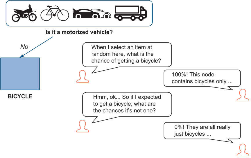
Figure 5.14 The left node is an example of a pure node, so there are no chances of selecting anything else.
To summarize, whenever you select anything from this node, it is a bicycle, and whenever you select a bicycle from this node, you can be sure about this instance’s class. This is because the classifier put nothing else under this node. It’s not surprising that the probability that the node contains instances of class(es) other than the class in question equals (1 - pclass,node). Table 5.2 lists the probabilities for all the classes in the left node.
Table 5.2 Summary of all class probabilities in the left node (first box)
Finally, let’s put these two components together. For each node, an impurity measure iterates over all classes in the dataset and considers how probable it is to randomly select an instance of a particular class from this node and, at the same time, how probable it is in this case that the instance is actually of any other class than the expected one. Put another way, we are estimating how probable it is that the classifier made a mistake by putting instances of other classes under the same node. Whenever we are talking about a probability of two things happening at the same time, in mathematical terms we mean multiplication. So, to derive the final measure of impurity for the left node, let’s apply the following equation:
Impurity_of_node =
sum_over_all_classes(probability_of_class_under_node *
                     probability_of_other_classes_under_same_node)
Let’s apply this formula to the left node:
Impurityleft = pmotorbikes,left*(1-pmotorbikes,left)
            + pbicycles,left*(1-pbicycles,left)
            + pcars,left*(1-pcars,left)
            + ptrucks,left*(1-ptrucks,left) =
            = 0*1 + 1*0 + 0*1 + 0*1 = 0
We started off saying that the leftmost node presents a case of a clear data separation, so its impurity should be the lowest (i.e., 0). Here we’ve got mathematical proof that this is indeed the case, as this calculation tells us that this node’s impurity indeed equals 0.
Let’s now look into the right node at the first level of the tree in figure 5.12. Going back to our boxes and toy models metaphor, let’s inspect the contents of the second box. After you applied a rule “Is it a motorized vehicle?” to the full set, it put 250 of the vehicles other than bicycles in the second box (and under the node on the right). This is a more challenging case, as this box contains a combination of 100 motorbikes, 100 cars, and 50 trucks, so we know from the start that it is not pure, and its impurity score should be greater than 0. Let’s derive this score step by step. First of all, let’s estimate the probability of randomly selecting instances of each class from this node. In other words, randomly pick models of a particular type out of the second box. Table 5.3 presents these probabilities.
Table 5.3 Probability estimation for the four classes in the right node (second box)
If you were to blindly pick a vehicle from the second box (or from under the right node), you would expect to end up selecting a motorbike 40% of the time (i.e., with a 0.40 probability), another 40% of the time you will expect to get a car, and in 20% of the cases it will be a truck. Now, say, you have blindly picked a toy model out of the box and expected to see a motorbike. According to the distribution of instances in this box, how often will it turn out to not be a motorbike? Figure 5.15 visualizes this.

Figure 5.15 Right node is an example of a less pure node: whenever you expect to get instances of a certain class, there are chances that you get instances of other classes instead.
As before, this equals to the probability of any class other than motorbike under this node, or (1 - pmotorbikes,right) = (1 - 0.4) = 0.60. Let’s summarize this for all classes in Table 5.4.
Table 5.4 Summary of all class probabilities in the right node (second box)
Finally, let’s calculate impurity of this node as before:
Impurityright = pmotorbikes,right*(1-pmotorbikes,right)
             + pbicycles,right*(1-pbicycles,right)
             + pcars,right*(1-pcars,right)
             + ptrucks,right*(1-ptrucks,right) =
             = 0.4*0.6 + 0*1 + 0.4*0.6 + 0.2*0.8
             = 0.64
If you continue estimating impurity of each of the nodes in the tree from figure 5.12 in the same way, you will end up with the impurity values shown in figure 5.16. It uses a more technical term for the node impurity estimations that we’ve just run—Gini impurity. Gini impurity is widely used in practice, and it is the value that is applied by the scikit-learn implementation of the Decision Trees algorithm that you will use for this task. The general formula for Gini impurity (GI) for a particular node i (e.g., left or right at a particular level) in a case that contains data from k classes (e.g., {motorbikes, bicycles, cars, trucks}) looks like that:
GIi = Σk,i probability_of_k_in_node_i * (1 - probability_of_k_in_node_i)Note that this is exactly the set of estimations that we used earlier.
Before we move on, here is a trick that will make estimations somewhat simpler and faster. Let’s denote probability_of_k_in_node_i as pk,i for brevity. When you calculate the Gini score over all classes in a node, you end up with the following components:
GIi = Σk,i (pk,i * (1 - pk,i)) = Σk,i pk,i - Σk,i (pk,i)2
Each node contains instances of some classes of vehicles. For example, the left node contains 100 bicycles out of the 100 instances it has, and the right node has 100 motorbikes and 100 cars out of 250 instances of vehicles it has, and then it also contains 50 trucks. So, whenever you look at the sum of the vehicles of all the classes under the same node (i.e., at Σk,i pk,i), they necessarily cover the total of all the vehicles in this node. There is simply no other way.

Figure 5.16 Impurity values (Gini impurity) for each of the nodes in the tree from figure 5.12
This means that for the left node Σk,i pk,i = Σk,left pk,left= 0 + 1 + 0 + 0 = 1, and for the right node Σk,i pk,i = Σk,right pk,right= 0.4 + 0.0 + 0.4 + 0.2 = 1 (i.e., you always end up with 1). So, you can rewrite the formula from earlier as
GIi = Σk,i (pk,i * (1 - pk,i)) = Σk,i pk,i - Σk,i (pk,i)2 = 1 - Σk,i (pk,i)2
Now it’s time to practice the skills you just acquired and calculate a GI score yourself.

Figure 5.17 Impurity values (Gini impurity) for each of the nodes in the tree from figure 5.13 (solution to exercise 5.6).
5.3.3 Selection of the best split in Decision Trees
Now that you have estimated the impurity of each node in each of the trees, how can you compare whole trees, and which one should the algorithm select? The answer is, at each splitting point, the Decision Trees algorithm tries to select the rule that will maximally decrease the impurity of the current node. In both cases, you start with the original dataset of 100 examples for 3 classes plus 50 examples for the fourth class. What is the original impurity of the topmost node, then?
GI(topmost node) = 1 - (3*(100/350)2 + (50/350)2 ) ≈ 1 - 0.265 = 0.735The tree from figure 5.12 produces two nodes at the first step. The left node of 100 out of 350 (2/7 of the dataset) instances with the GI of 0 and the right node of 250 out of 350 instances (5/7 of the dataset) with the GI of 0.64. The total impurity for this split (let’s call it split1) can be estimated as a weighted average where the weight is equal to the proportion of instances covered by each node:
GI(split1) = (2/7)*0 + (5/7)*0.64 ≈ 0.46Similarly, the tree in figure 5.13 produces two nodes at the first step. The left node of 200 out of 350 (4/7 of the dataset) instances with the GI of 0.5 and the right node of 150 out of 350 instances (3/7 of the dataset) with the GI of 0.45. The total impurity for this split (let’s call it split2) is then
GI(split2) = (4/7)*0.5 + (3/7)*0.45 ≈ 0.48Here is what happens when you apply the rule for split1: the impurity of the original set of instances drops from 0.735 down to 0.46. For split2, the impurity drops from 0.735 to 0.48. See figure 5.18 for a visualization.

Figure 5.18 split1 contributes to a comparatively larger gain in GI (0.275) than split2 (0.255).
Comparatively, split1 contributes to a larger gain. The difference between the original node impurity and the impurity of the produced nodes after split1 is 0.275 (i.e., 0.735 - 0.46), which is larger than the difference of 0.255 (i.e., 0.735 - 0.48) for split2. Even though the difference in this small example is not strikingly large, the classifier will prefer split1—the sequence of rules from figure 5.12 because they contribute to larger purity of the subsequent nodes. After all, the first rule applied in the tree in figure 5.12 successfully separates one of the classes (bicycles) from the rest of the data.
There are further parameters of the Decision Trees algorithm that you can control for. For instance, the tree in figure 5.13 is flatter than the one in figure 5.12, which will be selected based solely on the Gini impurity score. You can constrain the algorithm to build a tree of a particular depth, as well as containing up to a maximum number of nodes/leaves, which will also impact the order in which the rules are applied.
5.3.4 Decision Trees on language data
Now, let’s apply a Decision Trees algorithm to language data. See exercise 5.7 for another toy example based on authorship identification task. As before, try solving this exercise yourself before checking the solution, which is discussed immediately after the exercise.

Figure 5.19 An example of a decision tree built for a hypothetical set of 200 sentences from Jane Austen and 100 sentences from William Shakespeare. Only two rules are shown in this bit.
Let’s discuss the solution to this exercise. In this example, you start with a set of some 200 sentences from Jane Austen and 100 sentences from William Shakespeare. Application of the first rule, “Is there a word ‘happyer’?” allows you to set aside 50 sentences by William Shakespeare. But, as the word is spelled in the Early Modern English tradition, it doesn’t occur in any of the sentences by Jane Austen, so all 200 of them are shuffled to the right node at the first level of the tree. The second rule, “Is there a word ‘happiness’?” helps you identify 75 sentences from Jane Austen; however, none written by William Shakespeare contain a word with such a spelling. For brevity, only part of the whole tree is presented in this figure, so you can assume that there are many more rules applied at the later steps to the remaining set of 125 sentences by Jane Austen and 50 sentences by William Shakespeare. What are the Gini impurity scores for the nodes that are presented here? As before, you need to apply the Gini impurity calculation to each node using the formula
GIi = Σk,i (pk,i * (1 - pk,i)) = Σk,i pk,i - Σk,i (pk,i)2 = 1 - Σk,i (pk,i)2
This should give you the scores as presented in figure 5.20.

Figure 5.20 Gini impurity scores calculated for the tree from figure 5.19
This exercise may give you an idea as to why applying a Decision Trees classifier with all words as features and using thousands of rules in the form of “Is there a word X in this sentence?” would not be very efficient. With over 13,000 words in the vocabulary between the two authors, trees built that way would grow prohibitively large. From the algorithm’s efficiency point of view, there are two particular problems for decision trees: the prohibitively high number of features, and the fact that many words among this large number of features are very rare and will occur only in a few texts. This problem is called feature sparsity, and it means that the classifier will waste a lot of resources on features that are not very useful because they occur too rarely. This does not mean that the Decision Trees classifier is not applicable to this task; it only means that one needs to select appropriate features.
To wrap this chapter up, let’s apply the Decision Trees classifier to our task and compare the results to the benchmark model. NLTK has its own implementation of the Decision Trees algorithm, which you are going to use here. Since using all 13,553 words as features will slow the classifier down a lot, let’s select a smaller range of words that would make for promising features. This will be your first attempt at feature selection. A simple heuristic that works with selecting words as features is that those words that occur across most texts are not very informative, as they do not help distinguish between classes. At the same time, words that occur only in a few texts are not helpful either—even if they identify the author uniquely, they don’t occur frequently enough, so you might never see them again in any other text and thus they won’t help in practice. (This may remind you of the discussion on word importance based on word frequency from chapter 3—differences in word distributions are the motivation for term frequency and inverse document frequency measures.) Therefore, the best approach is to consider the middle range of word frequencies to generate the features.
Let’s start by estimating how often each word from the training set occurs across texts in this set—that is, let’s estimate document frequencies for all 13,553 words. Listing 5.10 shows how to do that. You start by importing Python’s Counter (https://docs.python.org/3/library/collections.html), which provides helpful frequency estimation functionality. Then you extract sets of words from each document. You need to use sets, since all you care about is whether a word occurs in a document and not how many times it occurs in a particular document. The “documents” in this task are, in fact, the sentences written by the authors. Therefore, you extract words from all sentences in the strat_train_set and apply Counter to calculate document frequency for each word in the training set. Finally, you print out the results.
Listing 5.10 Code to estimate document frequencies for all words in the training set
from collections import Counter              ❶

words = []

def extract_words(text, words):
    words += set([word for word in text])    ❷
    return words

for (sents, label) in strat_train_set:
    words = extract_words(sents, words)      ❸

counts = Counter(words)                      ❹
print(counts)                                ❺
❷ Extract sets of words from each document.
❸ Extract words from all sentences in the strat_train_set.
❹ Apply Counter to calculate document frequency for each word in the training set.
If you print out the results returned by this code, you will get a Python dictionary, where each word is assigned with its document frequency (i.e., the number of sentences in the training set, where it occurs). Here are the first few entries from this dictionary:
Counter({'.': 9108, ',': 7126, 'to': 4382, 'the': 4119, 'and': 3996,...As you can see, the most frequent word (full stop) occurs in 9,108 sentences in the training data, the next most frequent one (comma) in 7,126 sentences, and then the number of occurrences starts dropping quite quickly. In fact, if we visualize the number of document occurrences for all words, starting with the most frequent one (such word is technically said to be at rank 1 in the frequency table) and following with the descending order of frequencies (higher ranks), we will see a sharp drop, as the left plot in figure 5.21 shows. In practice, logarithmic function is often applied to raw frequencies to make the curve smoother and the changes in frequencies clearer. The right plot in figure 5.21 shows the same trend, but with the logarithm with base 10 applied to the absolute numbers.

Figure 5.21 Document frequencies for all words from the training set plotted against their ranks. The results for the word “happy” are marked with a cross on each graph.
To give you a more precise example, figure 5.21 also shows the position at which word happy can be found: it is the 217th most frequent word (thus, it has a rank of 217) and it occurs in 154 sentences in the training set. Document distribution of words in the training set is quite sparse. As many as 13,355 words occur in less than 0.0125% of the sentences (i.e., in less than 168 sentences each).
This skew in the distribution is not something specific to this particular task or dataset. It is an example of a common phenomenon in language data known as Zipf’s law (https://en.wikipedia.org/wiki/Zipf%27s_law). It was formulated by George Kingsley Zipf, and it states that the frequency of any word is inversely proportional to its rank in the frequency table. Originally, it states that the most frequent word will occur approximately twice as often as the second most frequent word, three times as often as the third most frequent word, and so on. The particular proportion is a rough estimate and depends on the data (e.g., in this case, you are looking into document rather than total word frequencies, so the ratio between the first and the second ranks is not exactly 1:2), but what matters is that the rank-frequency distribution is an inverse relation. In plain terms, this means that a small amount of very frequent words will occur in most documents, and a much larger number of words (so-called long tail of the word distribution) will be seen very rarely. This is exactly why you should apply frequency-based feature selection if you don’t want to overload your classifier with many relatively rare features.
Listing 5.11 selects words as features based on their distribution. It applies a threshold for the minimum and the maximum number of occurrences. For the minimum number of occurrences, a threshold of 200 sentences is used (i.e., a word is required to occur in at least 200 sentences to become a feature). The maximum threshold of 20% of the sentences is used in this code—that is, a word is required to occur in at most 20% (2,683) of all the sentences to be used as a feature. You may consider changing these thresholds, as they are used for the sake of the example only. Note that the maximum number of sentences in which a word may occur is 13,414, since this is the size of the training set. You store the words, whose distribution falls within the predefined range, in the selected_words list, and then you extract features from the sentences by including only the words that are contained in the selected_words list. This procedure is applied to all three datasets. Finally, you train the classifier and report the accuracy scores on each of the datasets.
Listing 5.11 Code to run DecisionTreeClassifier with the selected features
from nltk import DecisionTreeClassifier                            ❶

maximum = float(13414)                                             ❷

selected_words = []
for item in counts.items():
    count = float(item[1])
    if count > 200 and count/maximum < 0.2:                        ❸
        selected_words.append(item[0])
print(len(selected_words))

def get_features(text, selected_words):                            ❹
    features = {}
    word_list = [word for word in text]
    for word in word_list:
        if word in selected_words:
            features[word] = True
    return features

train_features = [(get_features(sents, selected_words), label)
                  for (sents, label)
                  in strat_train_set]
pretest_features = [(get_features(sents, selected_words), label)
                    for (sents, label)
                    in strat_pretest_set]
test_features = [(get_features(sents, selected_words), label)
                 for (sents, label)
                 in test_set]                                      ❺


classifier = DecisionTreeClassifier.train(train_features)          ❻

print (f"Accuracy on the training set = {str(classify.accuracy(classifier, train_features))}")
print (f"Accuracy on the pretest set = {str(classify.accuracy(classifier, pretest_features))}")
print (f"Accuracy on the test set = " +
       f"{str(classify.accuracy(classifier, test_features))}")     ❼
❶ Import NLTK’s DecisionTreeClassifier.
❷ The maximum number of sentences in which a word may occur is 13,414.
❸ Select words based on the minimum and the maximum occurrence thresholds.
❹ Extract features from the sentences by including only the words from the selected_words list.
❺ Extract features from all three datasets.
❼ Report the accuracy scores on each of the datasets.
This code returns an accuracy of around 81.00 on the training set, around 79.60 on the pretest, and around 80.70 on the test set. Figure 5.22 visualizes these results.

Figure 5.22 Accuracy scores on the training, pretest, and test sets with the Decision Trees classifier
Even though these results are lower than those obtained with the benchmark model, the model is remarkably consistent across all three datasets. This shows that the Decision Trees classifier generalizes well across the three datasets. In addition, it achieves relatively good results with a small subset of features. In fact, there are only 166 words that are selected as features by the code in listing 5.11, which is a much more compact feature space than the one that contains all of the 13,553 words as features. Chapter 6 will focus on the question of how you can find more informative and compact sets of features for language tasks.
Summary
-
Authorship attribution is concerned with identification of the precise identity of an anonymous author, while user profiling is concerned with profiling a broader set of users from various groups based on their writing. These two applications represent varieties of essentially the same task: our writing styles and word choices are typically very consistent, making it possible for automated algorithms to solve these tasks based on the characteristic features in writing.
-
Authorship attribution and user profiling are examples of tasks typically addressed with machine learning (ML) classifiers. Many NLP applications can be represented as supervised ML classification tasks, provided that you can define classes and features and provide high-quality data for the algorithms to learn from.
-
High-quality data is the key ingredient of a successful ML application. In case of authorship attribution and user profiling, we need texts annotated with the particular authors (or groups of authors). While such data may be hard to come by, literary works by famous writers are readily available, such as via Project Gutenberg.
-
The first steps in a machine learning pipeline include initialization of the data, extraction of the initial set of features, and setting up of the benchmark model. Naïve Bayes with words as features can be used as one of such benchmark models.
-
The true goal of machine learning is for the classifier to identify a set of characteristics pertaining to the task rather than the data. This helps ensure that the classifier learns about the task rather than memorizes the facts from the data, so it can generalize its knowledge well to any new test data. One way to check generalization behavior is to test your classifier on the data coming from the same source as the training data and compare its performance to that on the completely new data.
-
The ML toolkit scikit-learn provides you with implementations of a wide variety of classifiers and data processing techniques. In particular, it can be used to split the data into subsets representing a fair distribution of classes. If classes in your data are not represented in equal proportions, you need to apply the stratified shuffle split technique to learn about the actual, unbiased performance of your algorithm.
-
Unlike Naïve Bayes, the Decision Trees classifier tries to learn a sequence of rules that can split the data into pure sets of classes. Purity (or impurity) of the split can be measured quantitatively; for example, using Gini impurity score. In addition, purity scores are used across the board in machine learning, such as to select informative features for machine-learning classification other than decision trees.
-
One of the approaches to feature selection relies on the idea that the most informative words are neither very frequent, nor very rare. The results from the Decision Trees classifier show that it generalizes well, but there is still some room for improvement in terms of its performance.
Solutions to miscellaneous exercises
Suppose you had only two people on your contacts list. This means you have two “suspects” as the authors of the anonymous message you received. Each of them represents a particular class: Author1 or Author2, each with their own writing style. This makes it a binary task: the message is either produced by Author1 or Author2. This case can further be extended to as many authors (classes) as you have entries on your contacts list. In the case of user profiling, each class can be defined based on the particular groups of authors considered. For example, you can represent this as a binary problem for male versus female writers, or split the users into age groups—for instance 10-20, 20-30, 30-40 years old, and so on.
Chapter 2 presented an earlier example of an NLP task addressed with an ML approach that relied on word choice as features. Words are a good start. In the case of spam filtering, certain words like lottery signaled that the topic of the email is likely to be inappropriate for a work-related email. Words are useful as features in authorship attribution and user profiling, too—as we all have our favorites that we frequently use, they can signal who the author is. We will start with words as features in this task, and then we will explore the potential of other linguistic features.
You might notice that the first excerpt contains a word “receyue” that looks like a misspelled English word. This is actually how the word receive was spelled in Early Modern English, which might help you attribute the first piece of writing to William Shakespeare as the only author from this period of time. This sentence comes from his play Macbeth.
The second excerpt contains modern spelling of “receive,” so it is unlikely to originate from Shakespeare. However, unless you know about the favorite topics of the other writers or the names of the characters in their works, you might find this question challenging, so don’t worry if you didn’t get it right. This piece comes from Jane Austen’s Sense and Sensibility.
Now, what about the other two pieces? Do they come from any of the same authors, or are any of these pieces written by the other two writers? Can you see any similarities between the third and the fourth sentences and the first two?
In fact, the third piece also comes from Macbeth and the fourth from Sense and Sensibility, but don’t worry if you were not able to tell that. You may have spotted, however, an unusual spelling of “happyer” with y instead of i, which is another trait of Early Modern English. Note how in the fourth piece “happiness” is spelled in the more usual way.
Before you check the solution in the notebook, try coding it yourself. You need to apply the method cat_proportions to the test_set and add one more column to the results table. You might find out that the class proportions are not exactly the same in the test set as they are in the training and pretest sets; however, they are relatively similar and follow the same distribution trend. In real-life applications, you need to make sure that the training and test data have similar distributions, but it is hard to guarantee exactly the same class proportions.