
15
The m-Polar Fuzzy TOPSIS Method for NTM Selection
Madan Jagtap* and Prasad Karande
Mechanical Engineering Department, Veermata Jijabai Technological Institute, Mumbai, India
Abstract
The m-polar fuzzy set hybrid methods are the subjects of research. The applications of the m-polar fuzzy set hybrid methods are explored in different fields by researchers. One of the m-polar fuzzy set hybrid methodologies is m-polar fuzzy TOPSIS (a technique for order performance by similarity to ideal solution), used in industrial selection problems. In the paper, the nontraditional machining process (NTM) selection problem is solved with the m-polar fuzzy set TOPSIS method. Two criteria weight calculation methods are used while implementing the m-polar fuzzy set TOPSIS method; analytical hierarchy process (AHP) and Shannon’s entropy weight calculation methods are used. Effect of input data variation is analyzed on the Euclidean distance of alternatives from a positive ideal solution and Euclidean distance of alternatives from negative ideal solution for AHP weights and Shannon’s entropy weight, referred to as positive uncertainty and negative uncertainty. In this paper, results obtained with both ways are compared for rank performance. It can be concluded that there is no effect due to the change in the criteria weight calculation method on rank performance.
Keywords: TOPSIS, m-polar, MCDM, MCGDM, NTM
15.1 Introduction
The m-polar fuzzy set (mFS) algorithm was developed by Chen [1]. It solves multi-criteria group decision making (MCGDM) problems. The mFS is integrated with different multi-criteria decision making (MCDM) methods to form mFS hybrid methods. Hybrid approaches are developed and implemented by Akram [2, 3]. Some of the m-polar fuzzy set hybrid methods are mFS ELECTRE-I (elimination and et choice translating reality), mFS TOPSIS (a technique for order performance by similarity to ideal solution), etc. The mFS ELECTRE-I algorithm is implemented to single-valued input and validated for robot selection problems [16]. Researchers have developed their algorithms and implemented them to real-life issues from social and medical domains. This study’s motivation is to explore further these methods for engineering applications with slight changes in the algorithm. Criteria weight calculation methods are added for solving engineering applications. Analytical hierarchy process (AHP) and Shannon’s entropy weight calculation methods are used. This paper is divided into six headings. A literature survey follows the first heading in the introduction. The third heading consists of an explanation of methodology. The fourth heading is an industrial case study with its implementation. The non-traditional machining (NTM) process selection problem is considered for the performance of the mFS TOPSIS method. The fifth heading is the results and discussion. The final sixth heading is the conclusion and future scope.
15.2 Literature Review
The mFS TOPSIS (technique for order preference by similarity to ideal solution) methodology helps solve problems with the hesitant fuzzy set, applied to selecting a perfect brand name and selecting a suitable product design for a company [2]. A model for decision-making based on quality function deployment (QFD) in NTM processes selection was developed by Prasad [4]. Chakladar [5] solved four examples of NTM process selection with a diagraph based expert system. Preference ranking organization method for enrichment evaluation (PROMETHEE)-geometrical analysis for interactive aid (GAIA) method was studied and applied for selection of process, which gives a visual decision aid to decision managers [6]. Organization, Rangement Et Synthese De Donnes Relationnelles (ORESTE) method is helpful to analyze various industrial selection problems, which shows that it can effectively handle ordinal data for a given situation [7]. TOPSIS-AHP combined approach was used to solve the NTM process selection for the surface of revolution feature generation in stainless steel, also for efficient machining of precision holes on Duralumin (aluminium alloy), cylindrical through-holes generation on ceramic (non-conductive), and standard through-holes generation on Titanium [8]. The multi-objective optimization based on ratio analysis (MOORA) method implemented for solving complex problems of NTM process selection, MOORA method approach is robust and straightforward [9]. TOPSIS-AHP expert system developed by Choudhury [10] works efficiently for selecting a suitable NTM process in the surface of revolution on aluminium, considering a wide variety of attributes. Analytical network process (ANP) shows satisfactory results for setting appropriate NTM process with different materials and shape features as shown in Table 15.1.
Table 15.1 Comparison of different NTM process selection methods [11].
| Sr. no. | Name of method | Material and shape feature combination | |||
| Aluminium-surface of revolution | Ceramics-cylindrical through holes | Titanium-deep through cutting | Aluminium-precision small holes | ||
| 1 | AHP-based approach | ECM–PAM | USM–AJM–EBM– LBM | PAM–ECM–AJM | EBM–PAM–LBM |
| 2 | Diagraph-based approach | ECM–PAM | USM–AJM–EBM | PAM–EBM–AJM | EBM–AJM–PAM– CHM–LBM |
| 3 | ANP-based approach | ECM–PAM | USM–WJM–LBM– AJM–EBM | PAM–ECM– WEDM–WJM | WEDM–CHM– LBM–EBM |
Roy [12] has combined fuzzy-AHP and QFD techniques for selecting NTM process, fuzzy-AHP compared the importance of various NTM processes for product and process characteristics, and QFD gives final scores considering shape feature and material combination of NTM process. The Data envelopment analysis (DEA) assisted by multi-attribute decision making (MADM) method implemented to efficiently select suitable NTM processes for various shape features [13]. WASPAS (Weighted aggregated sum product assessment) and COPRAS (complex proportional evaluation assessment) methods were implemented in the NTM process selection for ceramic machining and found helpful in the application [14]. The case-based reasoning (CBR) approach was developed to select the NTM process, software was produced, and three different problems were cited to explain the potential of the CBR approach [15]. Variation in input data results in uncertainty is described by the framework [17]. Effect of normalization on mFS ELECTRE-I method was studied and found vector normalization as suitable normalization [18].
15.3 Methodology
15.3.1 Steps of the mFS TOPSIS
Let, A be the set of alternatives and V be the set of variables,
- Set of alternatives

- Set of variables
- Let, D be set of alternatives and variables, Decision Matrix

- W is the set of all the criteria weights obtained by either the AHP method or Shannon’s entropy weight calculation method,
Weights of criteria W = (w1, w2,w3, ……wk) where k = 1,2,3 …….q,
- F, is the weight multiplied decision matrix, Weight multiplied decision matrix
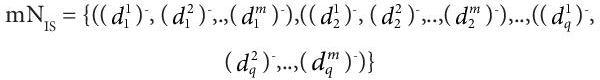
- The mF positive ideal solution and the mF negative ideal solution of alternatives, mPIS and mNIS are the positive ideal solution and negative ideal solution of alternatives
Where,

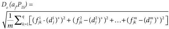
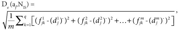
- Now, De (aj,PIS) be the positive euclidean distances of each alternative and De (aj,NIS) be the negative Euclidean distances of each option, which can be calculated as,
- The relative closeness-coefficient (RCC) of alternative can be computed as Ej be the RCC for option.
(15.5)
Alternatives with the highest RCC are considered the best alternative.
15.4 Case Study
To perform deep through cutting operations on titanium materials, eight NTM processes are available. Abrasive jet machining (AJM), ultrasonic machining (USM), chemical machining (CHM), electron beam machining (EBM), laser beam machining (LBM), electrochemical machining (ECM), electrical discharge machining (EDM), and plasma arc machining (PAM) are the processes available as alternatives. Two types of criteria are considered for the selection of a suitable NTM process, quantitative measures such as Tolerance and surface finish (TSF), Material removal rate (MRR), and Power requirement (PR). In contrast, the qualitative criteria are Cost (C), Shape factor (F), and work material type (M). A total of six criteria were considered for the selection process. The analytical hierarchy process (AHP) and Shannon’s weight calculation method are two different standards weight calculation methods. The analytical hierarchy process (AHP) is subjective, considering the expert decision for criteria weights. Shannon’s entropy weight calculation method uses data available from experiments for criteria weight calculations. The current case study will simultaneously implement the criteria weight calculation methods to analyse their effect on the m-polar fuzzy TOPSIS method for NTM process selection.
15.4.1 Effect of Analytical Hierarchy Process (AHP) Weight Calculation on the mFS TOPSIS Method
The analytical hierarchy process (AHP) weight calculation method is implemented to evaluate criteria weight for the decision matrix shown in Table 15.2. Below Table 15.2 shows readings for different criteria against the respective alternative NTM process.
Table 15.3 shows the normalized decision matrix obtained with the max linear approach. Again, the DM from Table 15.2 is considered for normalization purposes in Table 15.3.
AHP weight calculation performed for criteria weights, Table 15.4 shown below presents pairwise comparison of criteria.
The procedure for AHP weight calculation is done in Table 15.4. Table 15.5 below shows the rank of variables as per weight calculations.
Table 15.2 Decision matrix (DM), Example from [5].
| Sr. no. | NTM processes | TSF | MRR | PR | C | F | M |
| A1 | AJM | 2.5 | 0.8 | 0.22 | 1 | 1 | 4 |
| A2 | USM | 1.0 | 300 | 2.4 | 2 | 1 | 4 |
| A3 | CHM | 3.0 | 15 | 0.4 | 3 | 1 | 4 |
| A4 | EBM | 2.5 | 1.6 | 0.2 | 4 | 4 | 4 |
| A5 | LBM | 2.0 | 0.1 | 1.4 | 3 | 4 | 4 |
| A6 | ECM | 3.0 | 1500 | 100 | 5 | 5 | 4 |
| A7 | EDM | 3.5 | 800 | 2.7 | 3 | 1 | 5 |
| A8 | PAM | 5.0 | 75000 | 50 | 1 | 5 | 4 |
Table 15.3 Normalized DM with linear max N1 method [16].
| NTM | TSF | MRR | PR | C | F | M |
| A1 | 0.5 | 1.07E-05 | 0.0022 | 0.2 | 0.2 | 0.8 |
| A2 | 0.2 | 0.004 | 0.024 | 0.4 | 0.2 | 0.8 |
| A3 | 0.6 | 0.0002 | 0.004 | 0.6 | 0.2 | 0.8 |
| A4 | 0.5 | 2.13E-05 | 0.002 | 0.8 | 0.8 | 0.8 |
| A5 | 0.4 | 1.33E-06 | 0.014 | 0.6 | 0.8 | 0.8 |
| A6 | 0.6 | 0.02 | 1 | 1 | 1 | 0.8 |
| A7 | 0.7 | 0.010667 | 0.027 | 0.6 | 0.2 | 1 |
| A8 | 1 | 1 | 0.5 | 0.2 | 1 | 0.8 |
Table 15.4 Pairwise comparison matrix for criteria.
| TSF | MRR | PR | C | F | M | |
| TSF | 1 | 1/3 | 2 | 1/2 | 1/4 | 1/5 |
| MRR | 3 | 1 | 3 | 2 | 1/3 | 1/2 |
| PR | 1/2 | 1/3 | 1 | 1/2 | 1/4 | 1/5 |
| C | 2 | 1/2 | 2 | 1 | 1/3 | 1/4 |
| F | 4 | 3 | 4 | 3 | 1 | 1/2 |
| M | 5 | 2 | 5 | 4 | 2 | 1 |
Table 15.5 The rank of criteria based on weight their weights.
| Sr. no. | Variable | Priority | Rank |
| 1 | TSF | 0.0665 | 5 |
| 2 | MRR | 0.157614 | 3 |
| 3 | PR | 0.052616 | 6 |
| 4 | C | 0.095786 | 4 |
| 5 | F | 0.272725 | 2 |
| 6 | M | 0.354759 | 1 |
Consistency Ratio = 0.02949 and Principal Eigen Vector = 6.185. from the consistency ratio value, we can use the weights obtained from the AHP procedure for further steps. Table 15.6 is the weight multiplied matrix obtained by multiplication of AHP weights to normalization matrix shown in Table 15.3. For the remaining steps of the m-polar fuzzy TOPSIS algorithm, a weight multiplied matrix will be used.
Table 15.6 Weight multiplied matrix.
| NTM processes | TSF | MRR | PR | C | F | M |
| A1 | 0.03325 | 1.68632e-06 | 0.00011572 | 0.01914 | 0.05454 | 0.28376 |
| A2 | 0.0133 | 0.0006304 | 0.0012624 | 0.03828 | 0.05454 | 0.28376 |
| A3 | 0.0399 | 3.152e-05 | 0.0002104 | 0.05742 | 0.05454 | 0.28376 |
| A4 | 0.03325 | 3.35688e-06 | 0.0001052 | 0.07656 | 0.21816 | 0.28376 |
| A5 | 0.0266 | 2.09608e-07 | 0.0007364 | 0.05742 | 0.21816 | 0.28376 |
| A6 | 0.0399 | 0.003152 | 0.0526 | 0.0957 | 0.2727 | 0.28376 |
| A7 | 0.04655 | 0.00168112 | 0.0014202 | 0.05742 | 0.05454 | 0.3547 |
| A8 | 0.0665 | 0.1576 | 0.0263 | 0.01914 | 0.2727 | 0.28376 |
Table 15.7 Euclidean distance of alternatives from a positive ideal solution and negative ideal solution.
| Sr. no. | Euclidean distance of alternatives from PIS | Euclidean distances of alternatives from NIS |
| 1 | De (A1, PIS) = 0.295271 | De (A1, NIS) = 0.01995 |
| 2 | De (A2, PIS) = 0.293306 | De (A2, NIS) = 0.0191853 |
| 3 | De (A3, PIS) = 0.287005 | De (A3, NIS) = 0.0466147 |
| 4 | De (A4, PIS) = 0.192539 | De (A4, NIS) = 0.174547 |
| 5 | De (A5, PIS) = 0.196448 | De (A5, NIS) = 0.168565 |
| 6 | De (A6, PIS) = 0.17203 | De (A6, NIS) = 0.238597 |
| 7 | De (A7, PIS) = 0.276388 | De (A7, NIS) = 0.0872234 |
| 8 | De (A8, PIS) = 0.107636 | De (A8, NIS) = 0.275586 |
The positive ideal solution for the alternatives are shown below calculated with the help of equation 15.1,
The negative ideal solution for the alternative is shown below calculated with the help of equation 15.2,

Table 15.7, shown below, represents Euclidean distance for alternatives from a positive ideal solution and Euclidean distance for other options from the negative ideal solution obtained from equations (15.3) and (15.4), respectively.
Table 15.8 below shows the final ranking obtained from the RCC of each alternative, the highest the RCC higher will be the rank of other options.
Table 15.8 The rank of NTM processes using the m-polar fuzzy TOPSIS algorithm.
| Sr. no. | NTM process | Distance of alternatives from positive ideal solution with AHP weight | Distance of alternatives from negative ideal solution with AHP weight | Rank |
| 1 | AJM | 0.295271 | 0.01995 | Rank 7: E1,0.0632889 |
| 2 | USM | 0.293306 | 0.0191853 | Rank 8: E2,0.0613946 |
| 3 | CHM | 0.287005 | 0.0466147 | Rank 6: E3,0.139724 |
| 4 | EBM | 0.192539 | 0.174547 | Rank 3: E4,0.475493 |
| 5 | LBM | 0.196448 | 0.168565 | Rank 4: E5,0.461805 |
| 6 | ECM | 0.17203 | 0.238597 | Rank 2: E6,0.581055 |
| 7 | EDM | 0.276388 | 0.0872234 | Rank 5: E7,0.239881 |
| 8 | PAM | 0.107636 | 0.275586 | Rank 1: E8,0.719128 |
Figure 15.1, shown below, is the graphical representation of rank performance obtained by implementing m-polar fuzzy TOPSIS and AHP weight calculation method for selection of NTM process.
15.4.2 Effect of Shannon’s Entropy Weight Calculation on the m-Polar Fuzzy Set TOPSIS Method
Shannon’s entropy weight calculation method is implemented to evaluate criteria weight for the decision matrix shown in Table 15.1. Table 15.1 shows readings for different criteria against the respective alternative NTM process.
Table 15.10 shows the normalized DM obtained with the max linear approach. In addition, the DM from Table 15.9 is considered for normalization purposes in Table 15.10.
Shannon’s entropy weight calculation method is applied on decision matrix shown in Table 15.9, weight obtained fromShannon’s entropy weight calculation are as WTSF = 0.153523, WMRR = 0.200184, WPR = 0.182758, WC = 0.154599, WF = 0.157297, and WM = 0.151639. Table 15.11, shown below is weight multiplied matrix obtained with criteria weights given above and normalised decision matrix shown in Table 15.10.

Figure 15.1 Graphical presentation of the rank performance of alternatives for NTM selection with the m-polar TOPSIS and AHP weight calculation.
Table 15.9 Decision matrix, example from [5].
| Sr. no. | NTM processes | TSF | MRR | PR | C | F | M |
| A1 | AJM | 2.5 | 0.8 | 0.22 | 1 | 1 | 4 |
| A2 | USM | 1.0 | 300 | 2.4 | 2 | 1 | 4 |
| A3 | CHM | 3.0 | 15 | 0.4 | 3 | 1 | 4 |
| A4 | EBM | 2.5 | 1.6 | 0.2 | 4 | 4 | 4 |
| A5 | LBM | 2.0 | 0.1 | 1.4 | 3 | 4 | 4 |
| A6 | ECM | 3.0 | 1500 | 100 | 5 | 5 | 4 |
| A7 | EDM | 3.5 | 800 | 2.7 | 3 | 1 | 5 |
| A8 | PAM | 5.0 | 75000 | 50 | 1 | 5 | 4 |
Table 15.10 Normalized decision matrix with linear max N1 method.
| NTM | TSF | MRR | PR | C | F | M |
| 1 | 0.5 | 1.07E-05 | 0.0022 | 0.2 | 0.2 | 0.8 |
| 2 | 0.2 | 0.004 | 0.024 | 0.4 | 0.2 | 0.8 |
| 3 | 0.6 | 0.0002 | 0.004 | 0.6 | 0.2 | 0.8 |
| 4 | 0.5 | 2.13E-05 | 0.002 | 0.8 | 0.8 | 0.8 |
| 5 | 0.4 | 1.33E-06 | 0.014 | 0.6 | 0.8 | 0.8 |
| 6 | 0.6 | 0.02 | 1 | 1 | 1 | 0.8 |
| 7 | 0.7 | 0.010667 | 0.027 | 0.6 | 0.2 | 1 |
| 8 | 1 | 1 | 0.5 | 0.2 | 1 | 0.8 |
A positive ideal solution for the alternatives are shown below calculated with the help of equation 15.1,
Table 15.11 Weight multiplied matrix.
| NTM processes | TSF | MRR | PR | C | F | M |
| A1 | 0.07675 | 2.14e-06 | 0.00040194 | 0.0309 | 0.03144 | 0.12128 |
| A2 | 0.0307 | 0.0008 | 0.0043848 | 0.0618 | 0.03144 | 0.12128 |
| A3 | 0.0921 | 4e-05 | 0.0007308 | 0.0927 | 0.03144 | 0.12128 |
| A4 | 0.07675 | 4.26e-06 | 0.0003654 | 0.1236 | 0.12576 | 0.12128 |
| A5 | 0.0614 | 2.66e-07 | 0.0025578 | 0.0927 | 0.12576 | 0.12128 |
| A6 | 0.0921 | 0.004 | 0.1827 | 0.1545 | 0.1572 | 0.12128 |
| A7 | 0.10745 | 0.00212 | 0.0049329 | 0.0927 | 0.03144 | 0.1516 |
| A8 | 0.1535 | 0.2 | 0.09135 | 0.0309 | 0.1572 | 0.12128 |
A negative ideal solution for the alternative is shown below calculated with the help of equation 15.2,
Table 15.12, shown below, represents Euclidean distance of alternatives from a positive ideal solution and euclidean distance of alternatives from the negative ideal solution obtained from equations (15.3) and (15.4), respectively.
Table 15.13 below shows that the final ranking obtained from the RCC of each alternative, highest the RCC higher will be the rank of alternatives.
Figure 15.2, shown above, is the graphical representation of rank performance obtained by implementing m-polar fuzzy TOPSIS and Shannon’s entropy weight calculation method for selection of NTM process.
Table 15.12 Euclidean distance of alternatives from a positive ideal solution and negative ideal solution.
| Sr. no. | Euclidean distance of alternatives from PIS | Euclidean distances of alternatives from NIS |
| 1 | De (A1, PIS) = 0.333368 | De (A1, NIS) = 0.04605 |
| 2 | De (A2, PIS) = 0.334492 | De (A2, NIS) = 0.0311706 |
| 3 | De (A3, PIS) = 0.312123 | De (A3, NIS) = 0.0871168 |
| 4 | De (A4, PIS) = 0.286352 | De (A4, NIS) = 0.140036 |
| 5 | De (A5, PIS) = 0.294382 | De (A5, NIS) = 0.116888 |
| 6 | De (A6, PIS) = 0.207618 | De (A6, NIS) = 0.261007 |
| 7 | De (A7, PIS) = 0.30416 | De (A7, NIS) = 0.10322 |
| 8 | De (A8, PIS) = 0.156656 | De (A8, NIS) = 0.281378 |
Table 15.13 The rank of alternatives based on RCC.
| Sr. no. | NTM process | Distance of alternatives from positive ideal solution with Shannon’s entropy weight | Distance of alternatives from negative ideal solution with Shannon’s entropy weight | Rank |
| 1 | AJM | 0.333368 | 0.04605 | Rank 7: E1,0.12137 |
| 2 | USM | 0.334492 | 0.0311706 | Rank 8 : E2,0.0852441 |
| 3 | CHM | 0.312123 | 0.0871168 | Rank 6 : E3,0.218207 |
| 4 | EBM | 0.286352 | 0.140036 | Rank 3: E4,0.328424 |
| 5 | LBM | 0.294382 | 0.116888 | Rank 4: E5,0.284213 |
| 6 | ECM | 0.207618 | 0.261007 | Rank 2: E6,0.556963 |
| 7 | EDM | 0.30416 | 0.10322 | Rank 5: E7,0.253376 |
| 8 | PAM | 0.156656 | 0.281378 | Rank 1: E8,0.642366 |
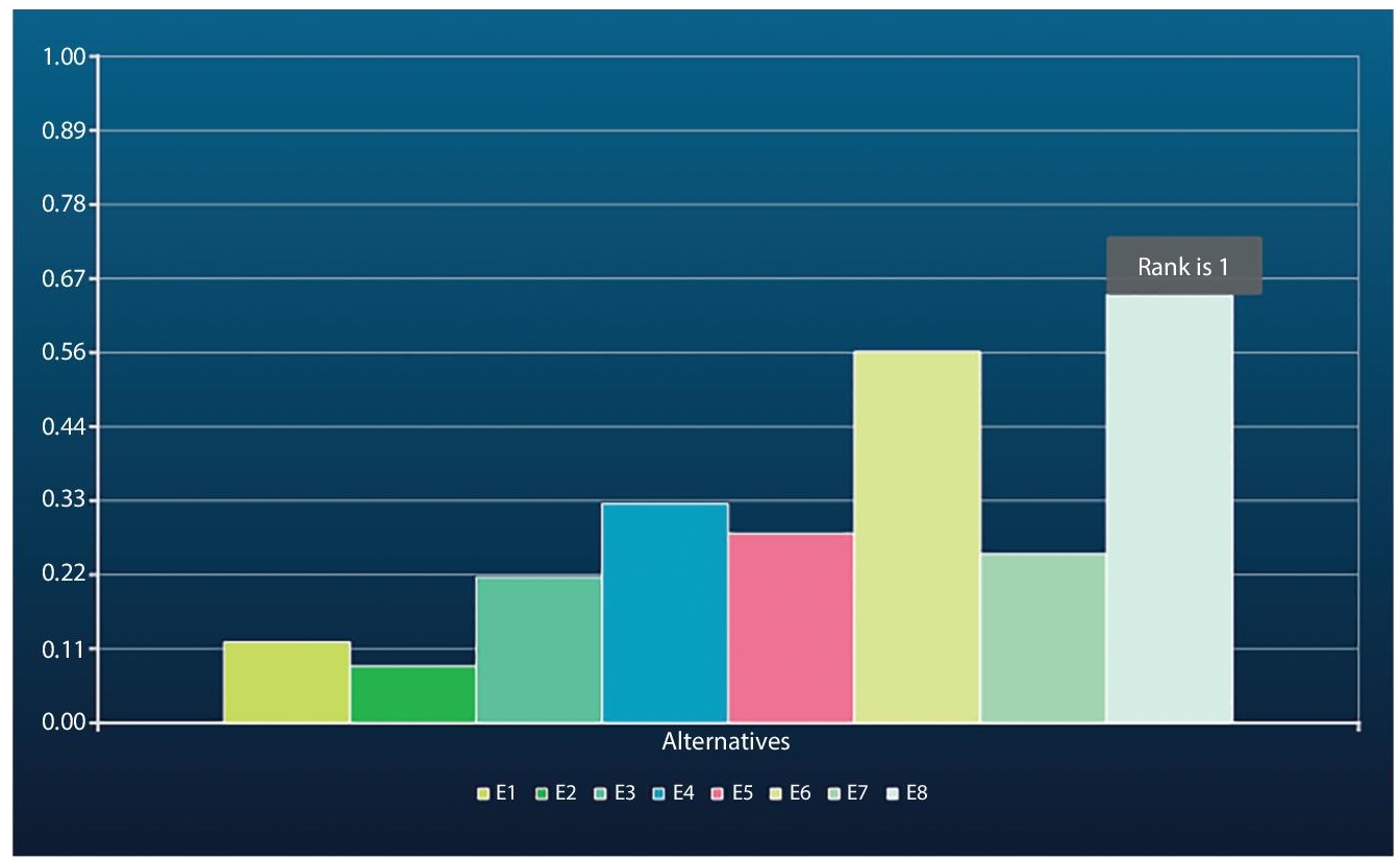
Figure 15.2 Graphical presentation of the rank performance of alternatives for NTM selection with the m-polar TOPSIS and Shannon’s weight calculation method.
15.5 Results and Discussions
Applied the m-polar fuzzy TOPSIS for single pole inNTM process selection first time and obtained the rank performance for deep through cutting in Titanium, the ranking is PAM-ECM-EBM-LBM-EDM-CHM-AJM-USM.
15.5.1 Result Validation
Results are validated with the help of previous research papers. Results obtained from the m-polar fuzzy TOPSIS method are compared to the diagraph based expert system and PROMETHEE-II approach. The best alternative from all the methods is the PAM process, while the second rank is given to the ECM process in the m-polar fuzzy TOPSIS and PROMETHEE-II methods. Table 15.14 below shows the comparison of rankings for different alternatives obtained from other methodologies.
As the rank performance obtained from the m-polar fuzzy TOPSIS using AHP weight calculations and Shannon’s entropy weight calculations are identical, there is a difference between positive and negative ideal solutions. Moreover, we get the difference between the distance of alternatives from the positive ideal solution obtained from the AHP weight calculation and Shannon’s entropy weight calculations. This difference is due to variation in the data input for the m-polar fuzzy TOPSIS method. It can be calculated for the distance of alternatives from negative ideal solution as well. Table 15.15 and Table 15.16 below give positive and negative uncertainty due to variation in data input.
Table 15.14 Result validation for m-polar fuzzy TOPSIS methodology with previous researchers work.
| Sr. no. | NTM processes | NTM processes rank with m-polar fuzzy TOPSIS | NTM processes rank with diagraph based expert system | NTM processes rank with PROMETHEE-II |
| 1 | AJM | 7 | 3 | 7 |
| 2 | USM | 8 | 5 | 4 |
| 3 | CHM | 6 | 7 | 6 |
| 4 | EBM | 3 | 2 | 5 |
| 5 | LBM | 4 | 4 | 8 |
| 6 | ECM | 2 | 6 | 2 |
| 7 | EDM | 5 | 8 | 3 |
| 8 | PAM | 1 | 1 | 1 |
Table 15.15 Data input uncertainty margin for a positive ideal solution with AHP and Shannon’s entropy weight calculation.
| Sr. no. | NTM process | Distance of alternatives from positive ideal solution with AHP weight (DPA) | Distance of alternatives from positive ideal solution with Shannon’s entropy weight (DPS) | Positive uncertainty (DPS-DPA) |
| 1 | AJM | 0.295271 | 0.333368 | 0.03840 |
| 2 | USM | 0.293306 | 0.334492 | 0.041186 |
| 3 | CHM | 0.287005 | 0.312123 | 0.025118 |
| 4 | EBM | 0.192539 | 0.286352 | 0.093813 |
| 5 | LBM | 0.196448 | 0.294382 | 0.097934 |
| 6 | ECM | 0.17203 | 0.207618 | 0.035588 |
| 7 | EDM | 0.276388 | 0.30416 | 0.027772 |
| 8 | PAM | 0.107636 | 0.156656 | 0.04902 |
Table 15.16 Data input uncertainty margin for a positive ideal solution with AHP and Shannon’s entropy weight calculation.
| Sr. no. | NTM process | Distance of alternatives from negative ideal solution with AHP weight (DNA) | Distance of alternatives from negative ideal solution with Shannon’s entropy weight (DNS) | negative uncertainty (DNS-DNA) |
| 1 | AJM | 0.01995 | 0.04605 | 0.0261 |
| 2 | USM | 0.0191853 | 0.0311706 | 0.01198 |
| 3 | CHM | 0.0466147 | 0.0871168 | 0.0405 |
| 4 | EBM | 0.174547 | 0.140036 | −0.03451 |
| 5 | LBM | 0.168565 | 0.116888 | −0.05168 |
| 6 | ECM | 0.238597 | 0.261007 | 0.02241 |
| 7 | EDM | 0.0872234 | 0.10322 | 0.01599 |
| 8 | PAM | 0.275586 | 0.281378 | 0.0057 |
15.6 Conclusions and Future Scope
The m-polar fuzzy TOPSIS method can be implemented to the NTM selection problem. It can be modified for single poles as shown and evaluated in case studies. AHP weight calculation and Shannon’s entropy weight calculations method do not affect the rank performance of alternatives. However, the effect of criteria weight calculation on a positive and negative ideal solution affects the euclidean distance of alternatives from a positive and negative ideal solution obtained due to input data variation. The term that shows these differences are referred to here as positive uncertainty and negative uncertainty. These uncertainties further show that Shannon’s entropy weight calculation is preferred over the AHP weight calculation as the relative closeness coefficient of alternatives is smaller in Shannon’s entropy weight calculation compared to the AHP weight calculation method. Further, this algorithm can be implemented for various industrial problems, such as robot selection, FMS selection, and RP selection.
References
- 1. Chen, J., Li, S., Ma, S., Wang, X., Polar fuzzy sets an extension of bipolar fuzzy sets. Sci. World J., 2014, Article ID 416530, 8, 2014.
- 2. Akram, M., Adeel, A., Alcantud, J.C.R., Multi-criteria group decision-making using an m-polar hesitant fuzzy TOPSIS approach. Symmetry (Basel), 11, 6, 1–23, 2019.
- 3. Akram, M., Waseem, N., Liu, P., Novel approach in decision making with m–polar fuzzy ELECTRE-I. Int. J. Fuzzy Syst., 21, 4, 1117–1129, 2019.
- 4. Prasad, K. and Chakraborty, S., A decision-making model for non-traditional machining processes selection. Decis. Sci. Lett., 3, 4, 467–478, 2014.
- 5. Das Chakladar, N., Das, R., Chakraborty, S., A digraph-based expert system for non-traditional machining processes selection. Int. J. Adv. Manuf. Technol., 43, 3–4, 226–237, 2009.
- 6. Karande, P. and Chakraborty, S., Application of PROMETHEE-GAIA method for non-traditional machining processes selection. Manage. Sci. Lett., 2, 6, 2049–2060, 2012.
- 7. Chatterjee, P. and Chakraborty, S., Advanced manufacturing systems selection using ORESTE method. Int. J. Adv. Oper. Manage., 5, 4, 337, 2013.
- 8. Chakladar, N.D. and Chakraborty, S., A combined TOPSIS-AHP-method-based approach for non-traditional machining processes selection. Proc. Inst. Mech. Eng. Part B J. Eng. Manuf., 222, 12, 1613–1623, 2008.
- 9. Chakraborty, S., Applications of the MOORA method for decision making in a manufacturing environment. Int. J. Adv. Manuf. Technol., 54, 9–12, 1155–1166, 2011.
- 10. Choudhury, T., Das, P.P., Roy, M.K., Shivakoti, I., Ray, A., Pradhan, B.B., Selection of non-traditional machining process: A distance-based approach. IEEE Int. Conf. Ind. Eng. Eng. Manage., 2013, 852–856, 2014.
- 11. Das, S. and Chakraborty, S., Selection of non-traditional machining processes using analytic network process. J. Manuf. Syst., 30, 1, 41–53, 2011.
- 12. Roy, M.K., Ray, A., Pradhan, B.B., Non-traditional machining process selection using integrated fuzzy AHP and QFD techniques: A customer perspective. Prod. Manuf. Res., 2, 1, 530–549, 2014.
- 13. Sadhu, A. and Chakraborty, S., Non-traditional machining processes selection using data envelopment analysis (DEA). Expert Syst. Appl., 38, 7, 8770– 8781, 2011.
- 14. Petković, D. and Radenković, G., Selection of the most suitable non-conventional machining processes for ceramics machining by using MCDMs. Sci. Sinter., 47, 2, 229–235, 2015.
- 15. Boral, S. and Chakraborty, S., A case-based reasoning approach for non-traditional machining processes selection. Adv. Prod. Eng. Manage., 11, 4, 311–323, 2016.
- 16. Jagtap, M. and Karande, P., Rank assessment of robots using m-polar fuzzy ELECTRE-I algorithm, in: Proceedings of the International Conference on Industrial Engineering and Operations Management, Bangalore, India, August 16-18, 2021.
- 17. Jagtap, M., Karande, P., More, N., Decision making framework considering uncertainty. Int. J. Adv. Sci. Technol., 29, 4, 7640–7649, 2020.
- 18. Jagtap, M. and Karande, P., Effect of normalization methods on rank performance in single-valued m-polar fuzzy ELECTRE-I algorithm. Materials Today: Proceedings, 2021.
Note
- * Corresponding author: [email protected]