CHAPTER 3
Computing Resources
Complex data analytics applications require multiple machines to work together in a reasonable amount of time. An application processing a large dataset needs to keep as much data as possible in the main memory of computers, but there are limits to a single machine, such as the amount of random access memory, hard disk space, and CPU power. As such, it is necessary to use many machines to execute applications when working on large datasets.
Nowadays even the tiniest home computer has multiple CPU cores, many gigabytes of memory, fast disks, and graphic processing units (GPUs). The simplest of programs use threads to utilize multiple CPU cores and thereby enhance the performance. In modern data centers, you will find powerful computers with many CPU cores, multiple GPUs, fast memory, and many disks.
Large computations need dedicated computing resources while they are executing. If critical resources such as a CPU core are shared between applications, they can see large performance reductions that are hard to investigate. To use the hardware resources efficiently for data analytics applications, we need deep knowledge about the inner workings of these resources and how they interact with each other.
Imagine we are starting with a data analytics project and bought a set of machines to store and process the data. The most probable first step would be to set up a distributed file system in the machines. Then it is time to develop and deploy the first programs to store the data and ideally get some insight. In the beginning, there are only a few applications, and they can be run one after another without interfering. All the machines are available all the time to execute the program as needed. As time goes on, people develop more applications that work on this data.
Now we need to coordinate between different developers to avoid executing the applications overlapping each other. If by accident two applications start to execute on the same resource such as a CPU, it can lead to an unexpected degradation in performance. Pinpointing the issue in a large set of machines can be difficult, as one overlapping computer may be causing a performance degradation for an entire application. To find the problem we may have to monitor the application in all the machines or send emails to all our co-workers asking whether they are also using the resources at the same time. Reasonably speaking, there is little chance of success pinpointing the problem in either case. And even if we do, we cannot guarantee it will not happen again in the future.
This has been an issue from the very beginning of cluster computing dating back to the 1980s. Eventually, computer scientists developed resource management software to efficiently allocate limited resources among applications. There are many forms of resource management software found in all types of large systems from clouds to high-performance computing systems. This software allocates computing resources to users or applications according to policies defined by organizations managing the resources and the application requirements. For example, when we request few virtual machines from a public cloud provider, a resource manager allocates them for a user. Application-level provisioners can be used after the resources are allocated or reserved for specific purposes. Apache Yarn is one example of an application-level resource manager for big data applications.
Data analytics frameworks hide the details of requesting computing resources and running applications on them. Application developers rarely need to consider the details of resource managers when designing. At the time of deployment, users can specify computing requirements of the application to the data analytics frameworks, which in turn communicate with the resource managers to satisfy those requests. Resource managers then make the scheduling decision of where to run the application by considering a range of factors such as computing nodes, racks, networks, CPUs, memory, disks, etc. Although most application developers are not concerned with the provisioning of resources for their applications, they should know about the type of computing environment in which the applications are deployed. There are many optimizations possible that can increase the efficiency of large-scale data applications by carefully considering the type of computing resources they use.
A Demonstration
As a test case, let's consider an application for detecting objects in images. Say we have a set of images and a few computers, and we want to develop an application that will efficiently identify objects in them, for instance, a car or a person. A simple application written using OpenCV, TensorFlow, and Python will satisfy this requirement. The most basic method is to run the resulting algorithm on a single computer as a sequential program that can go through images one by one in an input folder and label the objects in each.
The following is a simple Python program to detect objects in images using TensorFlow, Keras, OpenCV, and ImageAI libraries. This program assumes an
images
directory with images to examine and outputs the labeled images into an
output
directory.
from imageai.Detection import ObjectDetectionimport oscpath = os.getcwd()det = ObjectDetection()det.setModelTypeAsRetinaNet()det.setModelPath(os.path.join(cpath, "resnet50_coco_best_v2.0.1.h5"))det.loadModel()if not os.path.exists(os.path.join(cpath, "out")):os.makedirs(os.path.join(cpath, "out"))for f in os.listdir(os.path.join(os.path.join(cpath, "images"))):img_path = os.path.join(cpath, "images", f)out_path = os.path.join(cpath, "output", f)detections = det.detectObjectsFromImage(input_image=img_path,output_image_path=out_path)for eachObject in detections:print(eachObject["name"], " : ", eachObject["percentage_probability"])
The program can be executed simply by typing the following command:
$ python3 detect.py
If the computer that runs the algorithm has multiple CPU cores and enough memory (which will be the case even for low-end computers nowadays), we can start multiple instances of the program at once to speed up the object detection process. We then divide the images into multiple folders and start program instances manually pointing to these folders.
So far everything looks good for a lone machine. Now it is time to think about how to use the rest of our resources. The manual method comes to mind first, where we can duplicate the single machine approach across multiple instances. This will work on a small scale. But when the number of machines increases, this approach becomes much harder, to the point where a human can't keep up. This is where a script can help to automate the process. The script can log into each machine using a secure shell (SSH) connection and start the processes. The files must be in the local hard drives of each machine or placed in a distributed file system accessible to all.
ssh machineIP `cd program_folder && source venv/bin/activate && python detect.py` &
Multiple such commands for each machine can start and run our image detection program. Once the programs begin, scripts can check them for failures. If such a situation occurs without a mechanism to notify the user, the program may not produce the expected results.
This simple but important example assumes many things that can prove far more complicated in practice. For instance, most clusters are shared among users and applications. Some clusters do not allow users to install packages, and only administrators can install the required software. Even though our example is basic, we need to note that distributed programs and resource managers demand a more feature-rich version of what we have done so far.
Computer Clusters
Before the invention of the public cloud, clusters of physical machines were the only option to run distributed applications. Academic scholars used the supercomputing infrastructures provided by government agencies and universities. Companies had their clusters of machines to execute their applications, and most of the large computations were simulations. Some examples include physics simulations, biomedical simulations, and gene sequencing. These applications solve sets of mathematical equations by applying different optimization techniques. They start with relatively small amounts of data and can compute for days to produce answers even in large clusters. To run large applications, an organization needed to have an up-front investment of significant money and resources in the infrastructure.
With public clouds, large-scale computing is becoming a commodity where anyone can access a reasonably sized cluster in a matter of minutes to execute their applications. The previous model of dedicated physical machines is still used by government agencies and universities, as cloud performance for extreme-scale applications remains inadequate. Whether we are using public clouds or dedicated physical machine clusters, there are two broad situations in terms of application resource utilization. These can occur in either cloud environments or physical cluster environments.
In the case of a public cloud, we can allocate a set of machines to keep running a data cluster. This cluster can be used among many applications developed to work on this data. In such a case, it becomes a resource-sharing cluster. We can request a set of virtual machines every time we need to run an application. In this setting, it is a dedicated resource environment for the application.
The same applies to a physical machine cluster as well. We can purchase multiple machines to run a set of dedicated applications or share the physical cluster among many users, thus creating a resource-sharing environment. The latter is the mode used by supercomputers and large academic clusters. Organizations with requirements to host their own infrastructures can adopt either of these approaches depending on their applications.
There is a third option available for executing data analytics applications: cloud-based managed analytics engines. AWS EMR clusters and Google Cloud's cloud dataflow are examples of such managed clusters. Users are hidden from most of the details of the distributed environment, and only an application programming interface is exposed. These services use either dedicated clusters or resource-sharing clusters to meet the client's needs. However, in terms of understanding the underlying workings of data applications, this option is not relevant to our discussion.
Anatomy of a Computer Cluster
By definition, a computer cluster is a set of machines connected to each other by a network working together to perform tasks as if they are a single powerful machine. A computer in a cluster is often termed a node. Most clusters have a few machines dedicated to executing management-related tasks that are called head nodes or management nodes. The compute nodes do the actual computations. All nodes execute their own operating systems with their own hardware such as CPUs, memory, and disks. Often the management nodes and compute nodes have different machine configurations. Depending on the type of storage used, there can be dedicated machines for storing data, as shown in Figure 3-1, or storage can be built into the compute nodes, as shown in Figure 3-2. Usually, a dedicated network is used within the nodes of the cluster.

Figure 3-1: Cluster with separate storage

Figure 3-2: Cluster with compute and storage nodes
When assembling a cluster of machines in a public cloud, the storage can derive from a storage service offered by the cloud provider. The network can be shared among other machines not present in the cluster depending on the setting. In general, the topology of the networking and the location of the VMs are not visible to the user. Figure 3-3 shows a VM cluster setup with a storage service.
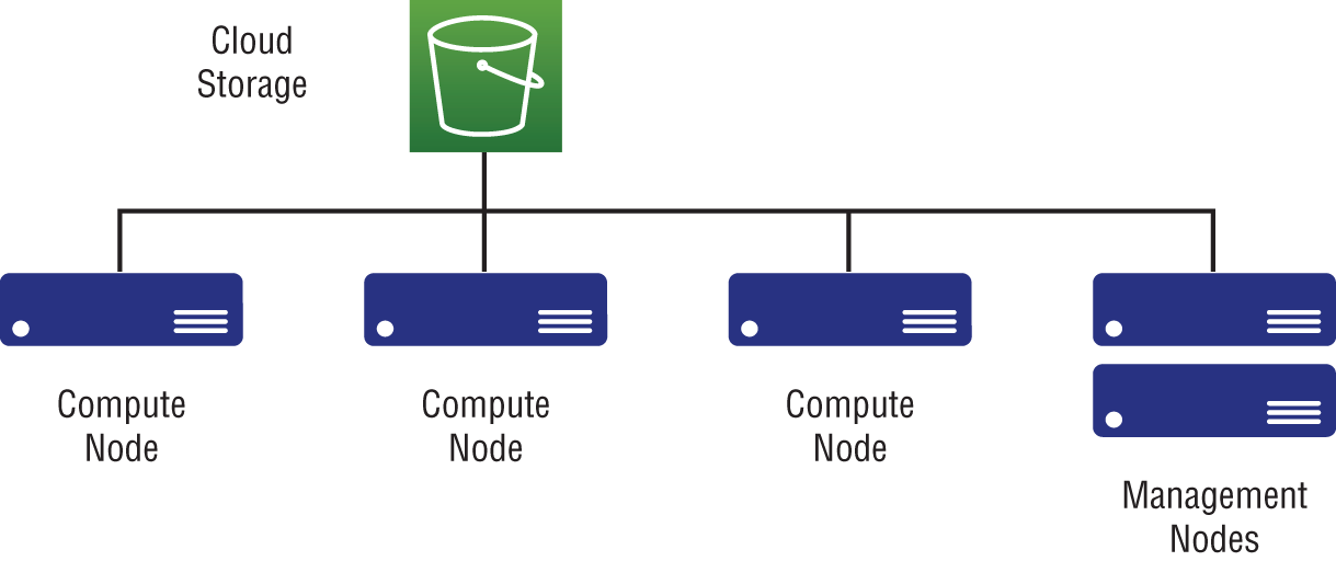
Figure 3-3: Cloud-based cluster using a storage service
SSH is the tool used to connect and execute commands in a cluster of machines. A user initially logs into a management node using an SSH connection. From there they can access the other nodes of the cluster. Depending on the access policies applied to the user, access can be restricted to other nodes. An application submitted to the cluster is called a job.
Data Analytics in Clusters
It is a long and complex undertaking to design, develop, and execute data analytics applications. This process involves data scientists, data engineers, and system administrators working together to create data analytics models that are then tested before being applied at a large scale. It is rare to see stand-alone data analytics applications without the support of distributed computing frameworks because of the complexities in developing them at a large scale. These frameworks provide APIs to program the applications and tools to execute and manage them. Once the applications are designed, they are further developed and tested in a local small-scale computer, such as a laptop, before being moved to larger environments like clusters and afterward into production clusters for even further testing.
Data frameworks supply different options for running applications depending on the nature of the resource-sharing environment. The dedicated cluster environment is the easiest to handle as it is not shared among many applications or users. We can think of a laptop as a dedicated resource environment for testing and development. Most frameworks provide a mechanism to run their applications in such a local environment. This mechanism is extended to run on a dedicated cluster as well. Table 3-1 shows some prominent data analytics frameworks along with options available to execute their applications on both shared and dedicated clusters.
Table 3-1: Data Analytics Frameworks and Resource Scheduling
| FRAMEWORK | DEDICATED CLUSTERS | SHARED CLUSTERS |
|---|---|---|
| Apache Spark | Runs with a main program and set of worker processes on worker nodes. These main program and worker nodes manage the Spark applications. | Yarn, Mesos, Kubernetes |
| Apache Flink | Starts a set of processes called manager and workers. These manage the applications. | Yarn, Kubernetes |
| Apache Hadoop | Yarn is the default mode; can run in master, worker as in Spark or Flink. | Yarn |
| OpenMPI | Stand-alone jobs using SSH to launch. | Sun Grid Engine (SGE), and the open-source Grid Engine (support first introduced in Open MPI v1.2) PBS Pro, Torque, and Open PBS LoadLeveler scheduler Slurm LSF Yod (Cray XT-3 and XT-4) |
Dedicated Clusters
At this point, we have seen systems adopting two approaches to start and manage applications. In the first one, every application is considered as stand-alone without any connection to other applications. The other method involves applications sharing resources in a dedicated environment using common processes. With this approach, applications for a particular framework have dedicated access, but alternative applications using the same framework can share the resources. Let's see how this approach is used in both classic parallel frameworks and big data frameworks.
Classic Parallel Systems
In classic parallel systems, an application is always thought of as a stand-alone entity. Here we see an example application and how it is run with four-way parallelism, first on a single node and then on two nodes. To run this program, we can install OpenMPI first:
$ sudo apt install libopenmpi-dev
Now we can use the following code written in C to run a test case. This program simply prints a message from each parallel process. Every process has a unique ID to distinguish itself from other processes.
#include <mpi.h>#include <stdio.h>int main(int argc, char** argv) {// Initialize the MPI environmentBatchTLink MPI_Init(NULL, NULL);// Get the number of processesint world_size;MPI_Comm_size(MPI_COMM_WORLD, &world_size);// Get the rank of the processint world_rank;MPI_Comm_rank(MPI_COMM_WORLD, &world_rank);// Print off a hello world messageprintf("Hello world from process id %d out of %d processors ", world_rank, world_size);// Finalize the MPI environment.MPI_Finalize();}
To compile the program we can use the following command assuming our program name is
task.c
.
$ mpicc.openmpi -o task task.c
Once compiled, the program can be run using the
mpirun
command:
$ mpirun -np 4 ./taskIt will give the following output:
$ Hello world from process id 1 out of 4 processors$ Hello world from process id 0 out of 4 processors$ Hello world from process id 2 out of 4 processors$ Hello world from process id 3 out of 4 processors
To run this example on two nodes, we need to install OpenMPI on both nodes and have
task.c
compiled and executable available on the same path for each. After meeting these requirements, we can use a file called
hostfile
to give the IPs/hostnames of the machines we are going to run on. Also, password-less SSH must be enabled on these hosts for the program to work across machines. The following is how a host file will look:
$ cat nodesexample.com.1 slots=2example.com.2 slots=2
The first part of each line is the IP/hostname of the node. The slots config indicates how many processors we can start on the given node; in our case we set it to 2. This number depends on the number of CPUs available and how we use the CPUs in each process.
mpirun -np 4 --hostfile nodes ./task
It will again give the same output but will run on two machines instead of a single machine.
Big Data Systems
Big data frameworks are taking a mixed approach for dedicated environments nowadays. Some provide stand-alone applications, while others offer mechanisms for sharing applications in a dedicated environment. Apache Spark is one of the most widely used big data systems, so we will select it as an example.
Apache Spark cluster utilizes a master program and a set of worker programs. The master is run on a management node, while the workers run on the compute nodes. Once these programs are started, we can submit applications to the cluster. The master and workers manage the resources in the cluster to run multiple Spark applications within a dedicated environment. Figure 3-4 shows this architecture; arrows indicate communications between various components.
Spark applications have a central driver program that orchestrates the distributed execution of the application. This program needs to be run on a separate node in the cluster. It can be a compute node or another dedicated node.

Figure 3-4: Apache Spark architecture
Here is a small hands-on guide detailing how to start a cluster and run an example program with Apache Spark:
## download and extract a spark distribution, here we have selected 2.4.5 version$ wget http://apache.mirrors.hoobly.com/spark/spark-2.4.5/spark-2.4.5-bin-hadoop2.7.tgz$ tar -xvf spark-2.4.5-bin-hadoop2.7.tgz## go into the spark extracted directory$ cd spark-2.4.5-bin-hadoop2.7## we need to change the slaves file to include the ip addresses of our hosts$ cp conf/slaves.template conf/slaves$ cat conf/slaveslocalhost# start the cluster$ ./sbin/start-all.sh# now execute an example program distributed with spark$ ./bin/spark-submit --class org.apache.spark.examples.SparkPi --master spark://localhost:7077 examples/jars/spark-examples_2.11-2.4.5.jar 100
It will give a long output, and there will be a line at the end similar to the following:
$ Pi is roughly 3.1416823141682313
In the case of Spark, we started a set of servers on our machines and ran an example program on it. By adding compute node IP addresses to the conf/slaves file, we can deploy Spark on multiple machines. Spark must be installed on the same file location on all the machines, and password-less SSH needs to be enabled between them as in the OpenMPI example. If we do not specify a master URL separately, it will start the master program on the node where we ran the cluster start commands.
Shared Clusters
As one might expect, resource-sharing environments are more complicated to work with than dedicated environments. To manage and allocate resources fairly among different applications, a central resource scheduler is used. Some popular resource schedulers are Kubernetes, Apache Yarn, Slurm, and Torque. Kubernetes is a resource scheduler for containerized application deployment such as Docker. Apache Yarn is an application-level resource allocator for Hadoop applications. Slurm and Torque are user-level resource allocators for high-performance clusters including large supercomputers. Table 3-2 shows popular resource managers, their use cases, allocation types, and units.
Table 3-2: Different Resource Managers
| RESOURCE SCHEDULER | USE CASES | ALLOCATION TYPE | ALLOCATION UNIT |
|---|---|---|---|
| Kubernetes1 | Enterprise applications and services, data analytics applications | Allocate a set of resources for applications | Containers |
| Slurm2 | High-performance clusters, supercomputers | User-based allocation of resources | Physical hardware allocation, containers |
| Yarn3 | Hadoop ecosystem-based applications | Application-level allocation | Physical hardware or virtual machine environments, containers |
The same examples can be executed on a cluster environment with some tweaks to the configurations and submit commands.
OpenMPI on a Slurm Cluster
To run the OpenMPI-based application on a Slurm cluster, the following commands can be used:
# Allocate a Slurm job with 4 nodes$ salloc -N 4# Now run an Open MPI job on all the nodes allocated by Slurm$ mpirun ./task
Note that we are missing the number of processes argument and the hostfile. OpenMPI knows it runs in a Slurm environment and infers these parameters from it. There are other ways to submit OpenMPI applications in a Slurm environment, such as using the batch command.
$ cat my_script.sh#!/bin/shmpirun ./task$ sbatch -N 4 my_script.sh$ srun: jobid 1234 submitted
Spark on a Yarn Cluster
The same Spark application can be executed on a Yarn cluster with minor modifications to the configurations and
submit
command. Note the master is specified as
yarn
, and the deploy mode is specified as
cluster
.
$ ./bin/spark-submit --class org.apache.spark.examples.SparkPi --master yarn --deploy-mode cluster examples/jars/spark-examples_2.11-2.4.5.jar 100
Distributed Application Life Cycle
Even though there are many types of hosting systems, including clouds, bare-metal clusters, and supercomputers, a distributed data application always follows a remarkably similar life cycle. The framework may choose different strategies to acquire and manage the resources depending on whether it is a resource sharing or dedicated resource environment. In a dedicated environment, distributed computing frameworks manage the resources and applications, whereas in shared environments the frameworks need to communicate with the resource managers to acquire and manage the required computing resources.
Life Cycle Steps
As we have seen in previous examples, it all starts at the command line with instructions to submit the application to the cluster. Sometimes frameworks provide UIs to submit applications. Once the command to submit an application is executed, the steps shown in Figure 3-5 are taken to distribute the application to the compute nodes. Following the application setup, a discovery step is used to figure out the details of various distributed parts of the application. The frameworks perform additional steps such as monitoring while the application executes.
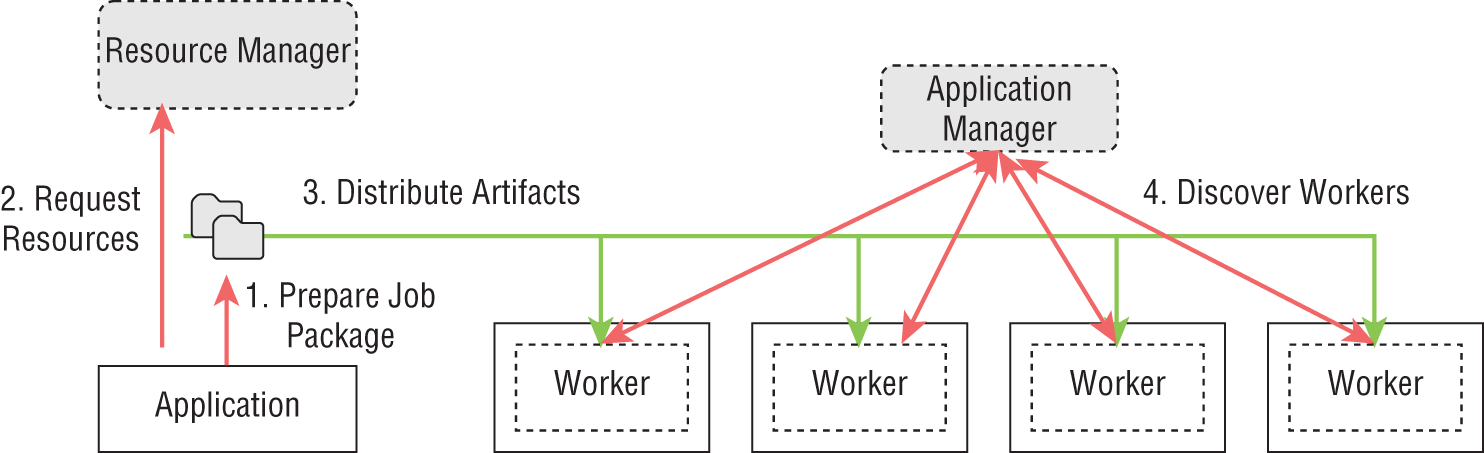
Figure 3-5: Life cycle of distributed applications
Step 1: Preparation of the Job Package
The framework prepares the job package to be distributed among the allocated machines. This step can execute additional validation steps to check whether the program is in an acceptable state to be submitted. In big data applications, the integrity of the dataflow graph is verified at this stage, and the availability of resources such as file paths can be checked.
The job package needs to be placed on different nodes to be executed. Various frameworks have specialized requirements in which the job needs to be formatted to run in these workers. For example, they may have a given folder structure with the executable in one folder, the dependencies of the application in another, and configurations in yet another. The job needs to be prepared according to a predefined format so that it can be placed on these workers to execute.
Step 2: Resource Acquisition
The program first requests resources from the cluster to execute. If the resources are not available at the time, the program is submitted to a queue where it waits until they are available. If the cluster cannot meet the requirements of the application, the application will be rejected. For example, should we request 1,024 CPU cores for an application when the cluster only has 512 CPU cores, that request cannot be satisfied and will fail.
There can be many policies set by administrators on the requirements of applications that can cause a rejection. In some resource managers, the application can request a time period for it to run. Since some clusters have limits on the number of hours an application can run, should the application exceed these limits it may not be granted resources.
Step 3: Distributing the Application (Job) Artifacts
At this point, the framework distributes the application artifacts to the allocated resources and starts executing the entry points of the program. In classic parallel systems, there is a distributed file system setup among the nodes. With a distributed file system, a separate distribution step is not necessary because files are accessible from all the nodes.
In cloud systems, this shared file system approach is uncommon, so the artifacts need to be distributed to all the machines. Some resource managers provide mechanisms to copy files to the allocated resources. Certain frameworks can utilize distributed file systems such as HDFS for file copying.
Step 4: Bootstrapping the Distributed Environment
In general, the locations (IP addresses) of the various parts of the program are unclear at the beginning of the program submission. Important information such as TCP ports used for communication between workers is similarly unknown. Given these conditions, bootstrapping a distributed application is a complex and time-consuming task, especially on a large scale.
To bootstrap, an application needs a process that has a known address (IP and port). This known point can be a central service such as a ZooKeeper, the submitting client, or a master program. Once the workers are spawned, they contact this known point to send their own information and discover information about other workers. This is a laborious operation when a very large number of parallel workers are involved (more than 10,000), and specialized hardware and algorithms can reduce the time required.
The processes started at the compute nodes are termed worker processes. These workers execute the actual program specified by the user and report their status to a master process for the particular job.
Step 5: Monitoring
An application needs to be monitored for faults and performance while it is running. Without monitoring, some parts of applications can fail without other parts knowing about it. Resource managers provide functions to keep track of applications. Application frameworks implement their own mechanisms for monitoring applications as well:
- Detecting failures—The program is monitored while it is executing to determine failures, performance issues, and progress. If a problem occurs, a recovery mechanism can be triggered to restart the program from a known previous state called a checkpoint. It is hard to detect failures in distributed environments. One of the most common methods is to rely on heartbeat messages sent from workers in a timely fashion. If a heartbeat is not received during a configured period of time, the worker is thought to be failed. The problem is that a worker can become slow and may not send the heartbeat message when needed, and the program can classify it as a failure when in reality it is not. Monitoring is a complicated aspect of keeping applications up and running.
- Collecting logs—Another common form of monitoring that occurs is collecting logs for determining the progress of the application. When hundreds of machines are involved in an application, they all can generate logs, and it is impossible to log into each of these machines to check for logs. In most distributed applications, logs are either saved in a distributed file system or sent to a common location to be monitored.
- Resource consumption—Cluster resource consumption can be monitored to see whether applications go over certain limits such as disk usage or memory usage and whether they encounter performance issues.
Step 6: Termination
After all the distributed computations complete, the application is stopped, the resources are deallocated, and the results are returned. When multiple machines and workers execute a distributed parallel application, there is no guarantee that every worker will stop at the same time. Distributed applications wait until all the workers are completed and then deallocate from the resource managers.
Computing Resources
Most of the computing power of the world is concentrated in data centers. These data centers provide the infrastructure and host the computing nodes to create public clouds, enterprise data warehouses, or high-performance clusters.
Data Centers
We are living in an age where massive data centers with thousands of computers exist in different parts of the globe crunching data nonstop. They work round-the-clock producing valuable insights and solving scientific problems, executing many exaflops of computations daily and crunching petabytes of data, consuming about 3 percent of the total energy used worldwide. These massive data centers host traditional high-performance computing infrastructures, including supercomputers and public clouds. The location of a data center is critical to users and cloud providers. Without geographically close data centers, some applications cannot perform in different regions due to network performance degradation across long distances.
A data center has many components, ranging from networking, actual computers and racks, power distribution, cooling systems, backup power systems, and large-scale storage devices. Operating a data center efficiently and securely while minimizing any outages is a daunting task. Depending on the availability and other features of a data center, they are categorized into four tiers. Table 3.3 describes the different tiers and the expected availability of data centers.
Table 3-3: Data Center Tiers
| TIER | DESCRIPTION | AVAILABILITY |
|---|---|---|
| 1 | Single power and cooling sources and few (or none) redundant and backup components | 99.671 percent (28.8 hours annual downtime) |
| 2 | Single power and cooling sources and some redundant and backup components | 99.741 percent (22 hours annual downtime) |
| 3 | Multiple power sources and cooling systems | 99.982 percent (1.6 hours annual downtime) |
| 4 | Completely fault tolerant; every component has redundancies | 99.995 percent (26.3 minutes annual downtime) |
Data center energy efficiency is an active research area, and even small improvements can reduce the environmental effects and save millions of dollars annually. A data center hosts computer clusters from a multitude of organizations. The individual organizations manage their computers and networking while the data center provides the overall infrastructure to host them, including connectivity to the outside world. Most data centers are built near the companies or the users they serve.
Power is one of the main expenses of running a data center. The availability of cheap power sources, especially green energy, is a big factor in choosing data center sites. Furthermore, places with low risk for natural disasters are chosen because it is costly to build systems that can withstand catastrophic events such as earthquakes or tsunamis. Cold climates can also reduce the cost of cooling, which is a big part of the overall power consumption for data centers. Table 3-4 shows some of the biggest data centers in the world and their power consumption.
Table 3-4: Massive Data Centers of the World
| DATA CENTER | LOCATION | SIZE | POWER | STANDARD |
|---|---|---|---|---|
| The Citadel4 | Tahoe Reno, USA | 7.2 million square feet | 650 MW | Tier 4 |
| Range International Information Group5 | Langfang, China | 6.3 million square feet | 150 MW | Tier 4 |
| Switch SuperNAP6 | Las Vegas, Nevada | 3.5 million square feet | 180 MW | Tier 4 |
| DFT Data Center7 | Ashburn, Virginia | 1.1 million square feet | 111 MW | Tier 4 |
Even though most of the online services we use every day are powered by data centers around the world, as users we rarely notice their existence. Application developers are also unaware of the physical locations of these data centers or how they operate. Nevertheless, they play a vital role in large-scale data analytics.
Physical Machines
Before clouds and VMs became mainstream, physical machines were the only choice for running applications. Now we need to rely on physical machines only rarely thanks to the ever-increasing popularity of public clouds, virtual machines, and containers. Physical machines are still used in HPC clusters due to performance reasons. Some high-performance applications need access to the physical hardware to perform optimally and cannot scale to hundreds of thousands of cores in virtual environments. Small-scale in-house clusters usually expose physical machines to the applications due to the complexity of maintaining private clouds.
The biggest advantage of physical machines is direct access to the hardware. This allows applications to access high-speed networking hardware, storage devices, CPU, and GPU features otherwise not available through virtualization layers. This allows applications written with special hardware features to achieve optimal performance. For mainstream computing, these features are not relevant as the cost of developing and maintaining such applications outweighs the benefits.
Network
The computer network is the backbone of a data center. It connects computers and carries data among them so applications can distribute functionality among many machines. Networks can carry data between data centers, within a data center, or simply within a rack of computers. Most data centers provide dedicated high-bandwidth connections to other data centers and designated areas. For example, the Citadel in Tahoe Reno provides 10Gbps network connections with 4 ms latency between Silicon Valley.
Within a data center, there can be many types of networks utilized by different clusters created by various companies. The machines are organized into shelves we call computer racks. A rack typically consists of many computers connected using a dedicated network switch. The network between racks is shared by multiple machines. Because of this, the networking speed is much higher in a rack than between machines of different racks.
Numerous networks are available nowadays, but the most notable currently deployed is Ethernet. In most cases, Ethernet runs at around 10Gbps, and there is hardware available that can deliver up to 100Gbps speeds. Specialty networks have been designed to run inside data centers such as InfiniBand, Intel Omni-path, and uGini. These networks provide ultra-low latencies and generally higher bandwidths compared to Ethernet. They are mostly used in high-performance computing clusters including large supercomputers and are considered a vital component in scaling applications to thousands of nodes and hundreds of thousands of cores. Because of their efficiency, more and more clusters in data centers are using such features to accelerate networking performance. Table 3-5 shows some of the fastest supercomputers in the world, their number of cores, and the network they use along with their performance.
Table 3-5: Top 5 Supercomputers in the World
| SUPERCOMPUTER | LOCATION | CPU CORES AND GPUS | PEAK FLOPS | INTERCONNECT |
|---|---|---|---|---|
| Fugaku8 | RIKEN Center for Computational Science Japan |
7,630,848 cores | 537 petaflops | Tofu interconnect D |
| Summit9 | Oak Ridge National Laboratory USA |
4608 Nodes, 2 CPUs per node. Each CPU has 22 Cores, 6 NVIDIA Volta GPUs per node. | 200 petaflops | Mellanox EDR InfiniBand, 100Gbps |
| Sierra – IBM10 | Lawrence Livermore National Laboratory USA |
4320 Nodes, 2 CPUs per node. Each CPU has 22 Cores, 4 NVIDIA Volta GPUs per node. | 125 petaflops | Mellanox EDR InfiniBand, 100Gbps |
| Sunway TaihuLight – NCRPC | National Supercomputing Center in Wuxi, China | 10.65 million cores | 125 petaflops | Sunway |
| Tianhe - 2A – NUDT | National Supercomputing Center in Guangzhou, China | 4.98 million cores | 100 petaflops | TH Express-2 |
Virtual Machines
The virtual machine (VM) was invented to facilitate application isolation and the sharing of hardware resources. Virtualization is the driving technology behind cloud computing, which is now the most dominant supplier of computation to the world. When utilizing a cloud computing environment, we will most probably work with virtual machines.
A virtual machine is a complete operating system environment either created on top of hardware directly or atop another operating system, as shown in Figure 3-6. The virtual machines we start on our laptops are running on our laptop OS. In production environments, they will be directly running on hardware using virtualization layers. The virtual machine is called a guest, and the actual machine that runs the VM is called the host.
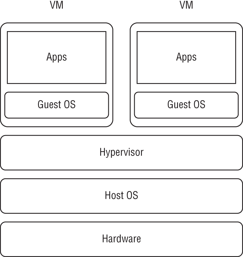
Figure 3-6: Virtual machine architecture
Containers
Containers operate in a lightweight virtual environment within the Linux operating system. Figure 3-7 shows a high-level architecture of containers where they run as a thin layer on top of the host operating system. Containers are lightweight compared to VMs because they do not run their own operating system kernel. This lightweight virtual environment is created mainly using Linux kernel cgroups functionality and namespaces functionality. Control groups are used to limit and measure the resources such as CPU or memory of a set of processes. Namespaces can be used for limiting the visibility that a group of processes has in the rest of the system.
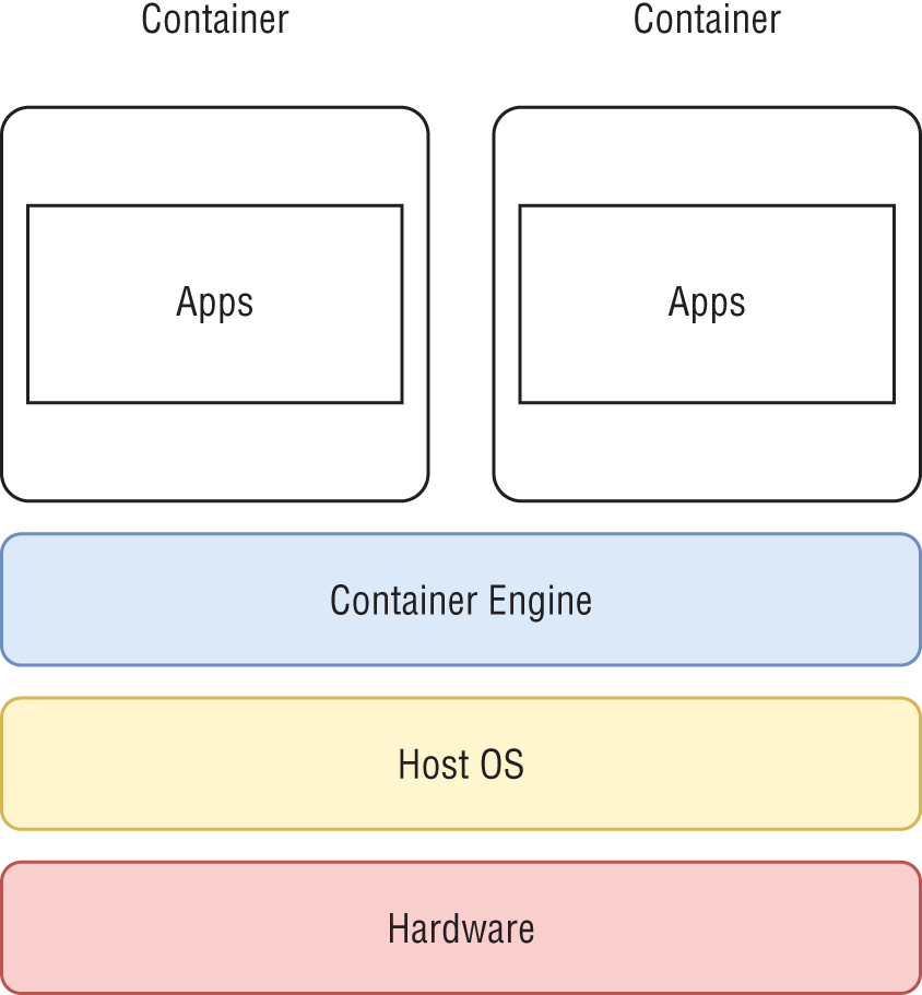
Figure 3-7: Docker architecture
By default, when we log into a Linux system, it has only one namespace that includes all the processes and resources. Linux processes start with a single process called
init
, and this process begins with other processes that may in turn start even more. As such,
init
is the common parent of all processes creating a single hierarchy or tree, all of which share the resources and can see each other.
With cgroups we can create process hierarchies that have limits on the resources they have available. We can allocate resources such as CPUs and memory to these process groups. The resource abstractions are called subsystems, examples of which include CPU, memory, network, and input/output (I/O). These subsystems control how the processes within a cgroup access the resources.
Namespace functionality facilitates deployment of process hierarchies with isolated mount points, process IDs, and networks. With namespace functionality, processes will see only the mount points created for them or the process IDs of the group. When enough of these limits and isolations are applied, we can create a totally isolated environment that does not interact with other processes of the system. This is the approach taken by container technologies such as Docker [1] and LXC.
Processor, Random Access Memory, and Cache
The CPU is the heart of a computer. For decades, a processing chip had only a single CPU core. Now single CPU core processors are almost nonexistent, and modern computers are equipped with chips that have multiple CPU cores. These are called multicore processors. A CPU core can execute a single thread (task) of the program at a time, and when many cores are available, it can execute tasks simultaneously. This allows programs to run in parallel within a single machine. Older computers with a single CPU provided the illusion of multitasking by rapidly switching between different threads of execution. With multicore processors, many threads of executions can truly occur on their own. A CPU core needs access to important structures such as the cache and memory to execute a program. In the days when chips contained only one core, caches and memory buses were all exclusive to that lone CPU. In modern multicore processors, some of these features are shared among multiple cores, while others are exclusive to each.
Apart from the CPU, random access memory (RAM) or main memory is the most important resource for data-intensive applications because of the amount of data being processed. RAM is expensive compared to other forms of storage such as disks. A single machine can have many memory modules that are connected to the CPU through memory buses. Imagine a processor with multiple cores and a single large memory connected to the processor with a single bus. Since every core requires access to the memory, they all need to share the same memory bus, which can lead to slower than average memory access speeds. Modern processors have multiple buses connecting numerous memory modules to increase the memory access times and bandwidth.
Accessing the main memory is a costly task for a CPU core because the memory bus is shared and because of the high number of CPU cycles required even with exclusive access. To reduce this access time, a much faster memory called a cache is used between the CPU core and the main memory.
Cache
It takes multiple CPU clock cycles to read an item from the main memory and load it to a CPU register. As a result, CPUs are equipped with caches, which are faster memory modules placed closer to the cores. The purpose of the cache is to reduce the average cost (clock cycles) required to access data from the main memory. These caches prefetch the most likely memory regions the CPU may use in future instructions. The CPU core can only access the memory in its cache, and when a memory request is made, it is first loaded into the cache and then served to the CPU core. If an item is not found in a cache, the CPU needs many clock cycles to fetch it from the main memory compared to loading it from the cache.
Modern computers have three caches called L1, L2, and L3, with L1 being closest to the CPU core. Figure 3-8 shows a cache hierarchy seen in modern processors. There are separate L1 caches for instructions to execute and find data. The fastest caches are the L1 instruction cache and L1 data cache. They are usually built near the CPU core in the same chip. These caches are equipped with fast memory and are expensive to build and hence limited in capacity. Next, there is the L2 cache, which is bigger than the L1 cache, and each core has one. Finally, there is an even larger cache called L3, which is shared among the cores of the chip.
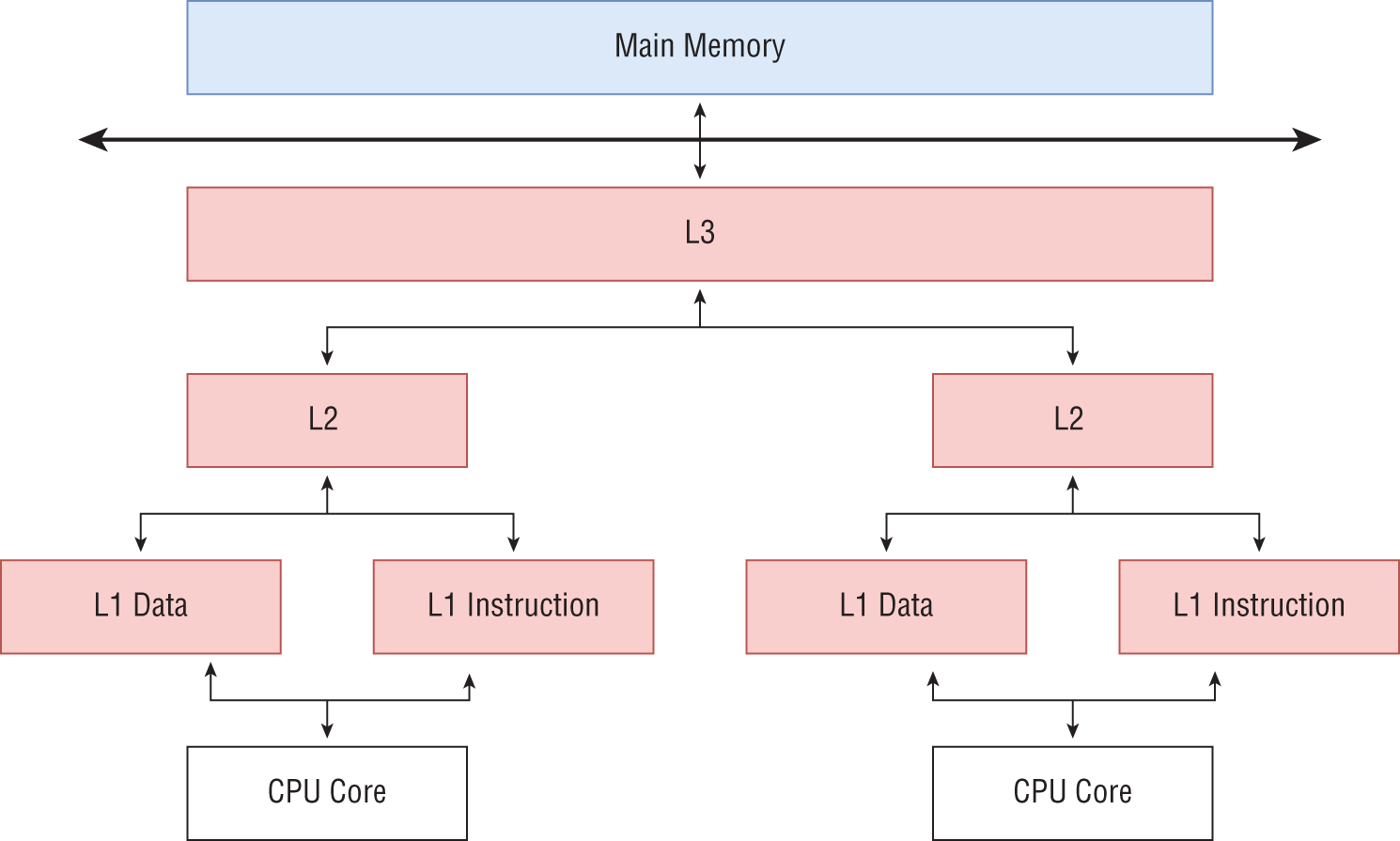
Figure 3-8: Hierarchical memory access with caches
We will look at the importance of cache for data-intensive application in later chapters.
Multiple Processors in a Computer
A computer can be built with numerous multicore processors in a single motherboard, most often referred to as multiple-socket computers. This allows more computing power to be packed into one node. When multiple CPUs are present, sharing memory I/O devices among different tasks running in them grows complicated. Certain architectures define how the resources are accessed in these configurations where a chip has multiple cores and there are several chips in a single machine. These are two popular architectures:
- Nonuniform memory access (NUMA)
- Uniform memory access (UMA)
It is important to understand these architectures to gain the best out of data-intensive applications. If programs are executed without considering these factors, serious performance degradation can occur.
Nonuniform Memory Access
NUMA is widely used in modern computers with multiple processors. In a NUMA computer, all the available memory is not uniformly (latency) accessible from a single core. The main memory is connected to the CPU cores using data buses. Each chip of a multiprocessor NUMA computer has its own memory buses to connect with memory modules. This means some memory is local to certain cores. The main memory, along with the cores and devices that are connected closely, are called a NUMA node. Different processor architectures may have one or multiple NUMA nodes per processor. Figure 3-9 shows a two-CPU configuration with two NUMA nodes.

Figure 3-9: NUMA memory access
When a CPU core tries to access memory that is located in another NUMA node, the access can be slower than its local memory access. To utilize the memory efficiently, the locality of the memory must be considered by the programs. Note that NUMA only affects the performance of an application, and no matter how the memory is allocated, its correctness will not be impacted.
NUMA memory locality is preserved by the operating system (OS) to some extent. When a process runs on a NUMA node, the OS will allocate memory for that process on its local memory. If there is no space in the NUMA local memory, the memory will be allocated in another NUMA node, slowing down the performance. Applications are scheduled on different cores and sockets by the OS throughout its lifetime. If an application is scheduled on one NUMA node and later scheduled on another node due to memory requirements, the program's performance can lag. Operating systems provide mechanisms to attach processes to NUMA nodes to prevent such performance issues.
Resource managers offer mechanisms to preserve NUMA locality while allocating resources to applications. For high-performance applications, such configurations need to be taken into account to achieve the best performance possible.
Uniform Memory Access
Uniform memory access remains uncommon and is available in only a few system architectures. Intel Xeon Phi is one such example. In a UMA system, the cores and processes access the main memory equally.
Hard Disk
Disks allow for much cheaper permanent storage of applications. There are mechanical hard disks, solid-state drives (SSDs), and NVMe SSDs available, with mechanical hard disks being the cheapest and NVMe SSDs being the priciest. Mechanical disks are also slower compared to SSDs, while NVMe provides the best performance.
Multiple hard disks can be grouped together to form a single logical disk using Redundant Array of Independent Disk (RAID) technologies to ensure fault tolerance and increased read/write performance. Depending on the RAID configuration, different aspects such as I/O performance or fault tolerance can be given priority. Computers configured to analyze large volumes of data are equipped with many hard disks and multiple I/O controllers to fully utilize the disks. Most organizations have data that need to be archived for potential future applications. Tape drives can offer economical storage for archiving such data, at the cost of slow read performances.
When data sizes are bigger than available memory, data applications need to use the hard disks for storing temporary data of computations. It is important to configure fast disks for such operations to perform optimally. Also, when multiple processes (threads) of a data analytics application access the same hard disk, it can reduce the performance. Hard disks are optimized for sequential I/O operations, so the applications should try to avoid random I/O operations as much as possible.
GPUs
Most of us are familiar with graphic processing units thanks to video gaming. Originally GPUs were created to relieve the CPU from the burden of creating images for the monitor to display. With the gaming industry's ever-increasing demand for realistic environments inside games, more and more computing power was added to GPUs. Unlike CPUs, GPUs are equipped with hundreds of cores and thousands of hardware threads that can manipulate large chunks of data simultaneously. Eventually scientists realized the GPU's potential to do large computations efficiently for dense matrix multiplications. Dense matrix multiplication is important for training deep neural networks. Now GPUs power numerous deep learning workloads, and large data analytics tasks are executed on them regularly.
Mapping Resources to Applications
In most frameworks, applications can request specific resource requirements. Usually these are the memory and CPUs. For example, an application can say it has 12 computing tasks (Map tasks) and each of them requires 8GB of memory and 1 CPU core to execute. The framework transfers these application-specific requirements to cluster managers when executing the application.
For data analytics application tasks, it is important to adhere to stricter resource mapping like NUMA boundaries to execute efficiently. Many frameworks allow finer-grained control over how the application processes are mapped to the resources. A user can request a parallel process to bind to a single CPU throughout its execution. By binding to a CPU core, an application can avoid unnecessary OS scheduling overheads and cache misses. Linux OS uses mechanisms to map specific resources to specific processes in order to achieve this level of control. When using cluster resource managers and frameworks, the users do not need to go to the Linux details and can instead apply these policies through various configurations.
Cluster Resource Managers
Efficient management of cluster resources is a topic all its own. Most mature cluster resource managers today offer equal functionality and performance. For the purpose of this textbook, we will not go into detail on how cluster resource managers are implemented but instead focus on their overall architecture and mechanics so that we can discuss them in the context of data analytics applications. Numerous such systems are available and at a glance their architecture and functionality are virtually identical. The details of their implementation can vary, but for the purposes of a data analytics application, they provide similar functionality with a common architecture. Because of this, by studying a few of them we can generalize the knowledge related to all. From a distributed application's perspective, a cluster resource manager performs three important tasks:
- Allocate resources for an application and give access to them. These resources can be any combination of containers, nodes, VMs, CPUs, memory, cache, GPUs, disk, or network.
- Job scheduling to determine which jobs run first (in case there are many jobs competing for resources) as well as determine the resources on which to run the jobs.
- Provide mechanisms to start and monitor distributed applications on these resources (life cycle management of the applications).
A resource provisioner has a set of server processes for managing cluster resources as well as interfacing with the users. To manage the actual compute nodes, daemon processes are started on each of them. The management servers and the processes run on the compute nodes communicate with one another. Additionally, the status of each process is monitored and reported to the management nodes. From the user side, there is a set of queues to submit applications, normally called job queues. These are used for prioritizing the jobs submitted by various users. An authentication mechanism can be used to distinguish and apply different capabilities to the users such as limits on the resources they can access.
Kubernetes
Kubernetes is a resource manager specifically designed to work with containers. When set up on a cluster of computers, it can spawn and manage applications running on containers. These applications can be anything, ranging from data analytics to microservices to databases. Kubernetes provides the infrastructure to spawn containers, set up auxiliary functions such as networking, and set up distributed storage for the spawned containers to work together. Some of the most important functions of Kubernetes include the following:
- Spawning and managing containers
- Providing storage to the containers
- Handling networking among the containers
- Handling node failures by launching new containers
- Dynamic scaling of containers for applications
Kubernetes supports the container technologies Docker, containerd, and CRI-O. Docker is the first container technology and made containers famous. CRI-O is a lightweight container technology developed for Kubernetes, and containerd is a simplified container technology with an emphasis on robustness and portability.
Kubernetes Architecture
Figure 3-10 shows the Kubernetes architecture. It has a set of servers that manages the cluster. These are installed on a dedicated server that does not get involved in executing the applications. There is also a set of worker nodes that run the actual container-based applications.
Management Servers
These are the features of management servers:
- API Server—This is a REST-based service that provides endpoints for clients to interact with the Kubernetes clusters. Client APIs are available in many different languages.
- etcd cluster—Kubernetes uses the etcd cluster to store the cluster state and metadata. Kubernetes uses a distributed coordinator called etcd that can synchronize various distributed activities among the worker processes.

Figure 3-10: Kubernetes architecture
- Controllers—Kubernetes runs many controllers to keep the cluster at a desirable state. The controller watches the state of the cluster and tries to bring it to the desired state specified by the user. The Deployment controller and Job controller are two built-in controllers available.
- Scheduler—Choose the compute resources to run the pods of an application.
Kubectl
This is a command-line tool provided by Kubernetes to interact with the cluster. The users connect to the Kubernetes API server to launch applications through the client API or using this command-line tool.
Worker Nodes
Each worker node runs kubelet process and the kube-proxy process. A worker node can be a virtual machine or physical node in a cluster.
- kubelet—This process manages the node and the pods that runs in that node. It accepts requests to start pods and monitors the existing pods for failures. It also reports to the controllers about the health of the node and the pods.
- kube-proxy—Handles individual subnetting within a node and exposes the services to external entities.
Kubernetes Application Concepts
There are many application specific features in Kubernetes. We will briefly look at some of the most relevant features for data intensive applications.
- Pod—This is the basic allocation unit in Kubernetes. A pod can run multiple containers, and an application can have multiple pods. It also encapsulates resources such as storage and network. A pod is a virtual environment with its own namespace and cgroups. So, pods are isolated from each other in a single node.
- Containers—Inside a pod we can run multiple containers. These containers can share the resources allocated to the pod. We run our applications inside the containers. A container packages the application along with its software dependencies.
- Volume—Volumes represent storage and are attached to a pod. A volume of a pod is attached to all the containers running inside that pod and can be used to share data within them. There are ephemeral volumes that are destroyed when pods exist. The persistent volumes retain data even if the pods are destroyed.
The original design goal of Kubernetes was to support more general forms of distributed applications such as web services. Container launching is still a time-consuming task compared to just launching processes in distributed nodes. With the support of major data processing platforms, Kubernetes is becoming a preferred destination for data analytics applications.
Data-Intensive Applications on Kubernetes
Now let us briefly examine how a data-intensive application will execute in a Kubernetes cluster without going into the details of any specific data-intensive framework. Because we are considering a distributed application, it will need multiple pods. Few of the pods will be dedicated to the management processes of our application, and the rest will run the computation in parallel. Most probably we will run one container per each pod. We are going to run each application in isolation without any connection to others in the Kubernetes cluster.
Container
Our container will be prepackaged with the framework software. We will need to transfer the job package to the container instances at runtime.
Worker Nodes
There are many controllers available in Kubernetes to create a set of pods that does the work in parallel. In a data-intensive application, these pods can run the worker processes that does the computations.
- Deployment—A configuration that describes the desired state of an application. Deployment controllers are used for updating pods and ReplicaSets.
- ReplicaSet—A ReplicaSet maintains a set of replica pods for long-running tasks. We can deploy a ReplicaSet as a deployment. Kubernetes will guarantee the availability of a specific number of pods at runtime.
- Job—A job consists of one or more pods that does some work and terminates. We can define how many pods to complete for a job to be successful. If this is not specified, each pod in the job will work independently and terminate.
- StatefulSets—This controller manages a set of replica pods for long-running tasks with added functionality such as stable unique network identifiers, stable persistent storage, and ordered graceful deployments and scaling.
Because of the added functionality, let's assume we are going to use a StatefulSet for our worker nodes. We will mount an ephemeral volume for workers to keep the temporary data.
Management Process
This process is responsible for coordinating the worker nodes. For example, it can tear down the application when it is completed and provide functions to handle failed worker processes. We can use a StatefulSet to start the management process because it provides a unique IP for other workers to connect.
Workflow
When a user submits a job package to run, we will first start the management process as a StatefulSet. After it is started, we can start the StatefulSet for worker processes by giving the IP address of the management process. Before the worker processes start, they need to wait for a copy of the job package to the containers. We can use the Kubernetes functions to copy the job package from client to the containers.
Once the pods are started, the workers will connect to the management processes. They will do a discovery step to find the addresses of other processes with the help of the management process. Once they know the IP addresses of others, they can establish network connections.
At this point, worker processes can start running the parallel application. Once they are done with executing the code, they can send a message to management process, which will terminate the pods by asking the Kubernetes.
There are many choices for executing a data-intensive application on top of Kubernetes at each step we described. What we described here is a great simplification of an actual system, but the core steps will be similar.
Slurm
Slurm [2] is a widely used resource manager in high-performance clusters, including the largest supercomputers. Slurm works by allocating physical resources to an application. These can be anything, from compute nodes to CPUs or CPU cores, memory, disks, and GPUs. Slurm has a similar architecture to Kubernetes with a set of servers for managing the cluster and daemon processes to run on the cluster nodes. As shown in Figure 3-11,
slurmctld
is the main process that manages the cluster, and
slurmdbd
is for keeping the state of the cluster persistent to a database. The
slurmd
daemons run on the compute nodes managing the resources and the processes spawned on them.

Figure 3-11: Slurm architecture
Slurm provides an API and a set of command-line utilities wrapping these APIs to interact with it. Command-line utilities are the preferred choice for most users to interact with Slurm. Slurm supports allocations both in batch and interactive modes. In interactive mode, once resources are allocated, users can SSH to them and execute any processes they might need. In the batch mode, a distributed application is submitted up front and run by Slurm. Due to human involvement, interactive mode does not use the resources very efficiently. Many production clusters only allow batch submissions in the main compute nodes and permit interactive jobs on just a small number of nodes for debugging purposes.
Slurm has different built-in job scheduling algorithms. There are API points to define custom algorithms as well. By default, Slurm uses a first-come, first-serve job scheduling algorithm. Other algorithms such as Gang scheduling and backfill scheduling are available as well.
Yarn
Yarn was the first resource scheduler designed to work with big data systems. It originally derives from the Hadoop project. Initially Hadoop was developed with resource management, job scheduling, and a map-reduce application framework all as a single system. Because of this, Hadoop did not have a mechanism to work with external resource managers. When Hadoop was installed on a cluster, that cluster could only be used to run Hadoop applications. This was not an acceptable solution for many clusters where there were other types of applications that needed to share the same resources.
Yarn decoupled the resource management and job scheduling from map-reduce applications and evolved as a resource scheduler on its own for big data applications. MapReduce became another application that uses Yarn to allocate resources. As one might expect, Yarn has a similar architecture to Kubernetes and Slurm where there is a central server called ResourceManager and a set of daemon processes called NodeManagers that run on the worker nodes.
An application in Yarn consists of an application manager and a set of containers that runs the worker processes. A data analytics framework wanting to work in a Yarn environment should write the application manager code to acquire resources and manage the workers of its applications. Figure 3-12 shows this architecture with two application managers running in the cluster.
Similar to Slurm, Yarn has a queuing system to prioritize jobs and various scheduling objectives can be applied to the applications. One of the most popular considerations in Yarn applications is the data locality. Yarn also implements various job scheduling algorithms [3] such as fair scheduling and capacity scheduling to work in different settings.
Job Scheduling
The goal of a job scheduling system is to allocate resources to users or applications in the most efficient way possible. In a cloud environment, the objective may be to minimize the cost while maximizing performance. In a research cluster, one might aim to keep the cluster fully utilized all the time. This presents unique challenges for the algorithms created to schedule the workloads on such clusters. Most application developers do not need to fully understand the details, and as such they are sometimes not visible to them. For example, when we request a set of VMs from a public cloud provider to run our application, the cloud provider considers many factors before deciding what physical nodes to use for creating the VMs.

Figure 3-12: Yarn architecture
A job scheduling system takes a set of jobs as input and outputs a job schedule, which indicates the order of the jobs as well as the specific resources for each job. It is often a challenge to find the best schedule in a reasonably complex system with many jobs competing for resources. Most algorithms make assumptions and lower the requirements to tackle the problem in a finite period as there is no point in devoting a large amount of time to finding the best schedule while your resources are idling.
A scheduling system consists of three parts: a scheduling policy, objective functions, and scheduling algorithms [4]. The scheduling policy states high-level rules to which the system must adhere. The objective function is used to determine a particular job schedule's effectiveness. The algorithms incorporate the policies and objective functions to create the schedule.
Scheduling Policy
A scheduling policy dictates high-level requirements such as what type of resources are accessible to which users and priority of different applications. Say, for instance, we take a data analytics cluster that runs jobs each day to determine critical information for an organization. This cluster is also shared with data scientists who are doing experiments on their newest machine learning models. The organization can define a policy saying the critical jobs need to run no matter what state the cluster is in. When this policy is implemented, an experimental job run by a data scientist may be halted to run a higher priority job, or it may have to wait until the higher-priority jobs complete.
So, a scheduling policy contains a set of rules that specifies what actions need to be taken in case there are more resource requests than available.
Objective Functions
An object function determines whether a resource schedule is good or bad. Objective functions are created according to the policies specified by the organization. A cluster can run many jobs at any given time. These applications demand various resource requirements (number of processors, nodes) and execution times. At any given time, the free resources of a cluster can be scattered across many racks of nodes. Furthermore, some applications can benefit from special hardware support and placement of the worker processes. These requirements can be specified with the job scheduling algorithms to make better decisions about where to place applications. We can look at few common objective functions used in resource schedulers.
Throughput and Latency
Throughput and latency of the system are two main metrics used to determine the quality of a scheduling system. Throughput is measured as the number of jobs completed within a given period. Latency can be taken as the time it takes to complete jobs.
Priorities
Algorithms can take the priorities of applications into account when scheduling. Usually, priorities are configured with different job queues. Jobs submitted to queues with higher priorities are served first. For example, when used with Gang scheduling, the higher-priority jobs will get more execution time compared to the lower-priority ones.
Lowering Distance Among the Processes
A scheduling algorithm can try to lower the distance between various parts of an application in terms of networking to improve its performance. Slurm uses the Hilbert space-filling curve [5] to order nodes to achieve good locality in 3D space. The Hilbert curve fitting method transforms a multidimensional task allocation problem into a one-dimensional space, assigning related tasks to locations with higher levels of proximity. Lowering the networking distance can greatly increase the efficiency of network I/O-intensive programs.
Data Locality
Data locality–aware scheduling is common in big data schedulers like Yarn. It applies to clusters with computing and storage cohabited in the same nodes. A prime example is an HDFS cluster. A scheduler tries to minimize the distance between the data and the computing as much as possible. If all the cluster nodes are available, this means placing the application on the same nodes where the data is present. If the scheduler cannot run the application on the nearest nodes, it can instead place them on the same racks as the data.
When many jobs are running on a cluster, it is impossible to completely guarantee data locality. Data can be spread across more nodes than the number requested by the application, or the application may ask for more nodes than the nodes with the data. Other applications might also be executing on the nodes with the data.
Data locality was much more important in the early days of big data computing when the network was vastly slower than reading from the hard disk. By contrast, nowadays networks can be many times faster. In cloud systems, data is stored in services such as S3. As such, data locality is not as important as it was before.
Completion Deadline
Some jobs need to run within a given deadline to be effective. The resource scheduler needs an approximate time of completion from the user to achieve this. Usually, we know the time to run an application with a set of given parameters and resources from prior experience of running it. Resource schedulers do not try to allocate more resources (increase parallelism) on their own to finish a job quickly as it can decrease performance in some applications.
Algorithms
The goal of a scheduling algorithm is to select which jobs to run when the demand is higher than the available resources. The algorithm should select the jobs such that it creates a good schedule according to the objective functions defined. If we can run every job immediately because there are resources available, we do not need to use these algorithms.
There are many scheduling algorithms available in the literature. In practical systems, these algorithms are adapted to support various objective functions according to the applications they support.
First in First Out
First in First Out (FIFO) is the most basic scheduler available in almost all systems. As the name suggests, jobs are executed in the order they are submitted. It is simple to understand and works with systems that have relatively less work compared to the resources available, although it can lead to idle resources and low throughput. We will see an example later with the backfill scheduling algorithm.
Gang Scheduling
Gang scheduling is a technique used for running multiple applications on the same resources simultaneously by time sharing between them. In this case, applications are oversubscribed to the resources, and they must take turns executing like in OS threads. To achieve gang scheduling, the resources required by all applications running on a single resource must be less than its capacity. An example is a temporary hard disk space used by applications. If the requirement of all the applications running simultaneously is bigger than the capacity of the hard disk, gang scheduling will fail. Another such resource is the RAM used by the applications.
Gang scheduling allows a scheduler to improve responsiveness and utilization by permitting more jobs to begin executions faster. Shorter jobs can finish without waiting in queues for longer jobs to terminate, increasing the responsiveness of the overall cluster.
List Scheduling
This is a classic and simple scheduling technique where it runs the next job that fits the available resources. Because of its simplicity, it can be implemented efficiently and even provides good schedules in practical systems.
Backfill Scheduling
The backfilling [6] algorithm tries to execute jobs that are ahead in the job queue in case it cannot execute the head of the queue due to resources not being available. When it picks a job that is down in the queue, it tries not to postpone the job at the head of the queue. This requires knowledge of the job execution times for each job.
Figure 3-13 shows the difference between FIFO and backfill scheduling. Imagine we have two resources (r) and four jobs. Jobs 1 to 4 take resources and time pairs of Job1 - {r = 1, t = 2}, Job2 - {r = 1, t = 4}, Job 3 - {r = 2, t = 3}, Job 4 - {r = 1, t = 2}. These are submitted in the order of 1 to 4. If we strictly follow the FIFO schedule, Job 4 needs to wait until Job 3 is completed. With backfill scheduling, we can start Job 4 after Job 1 completes. Note that the Job 3 start time does not change because of this.
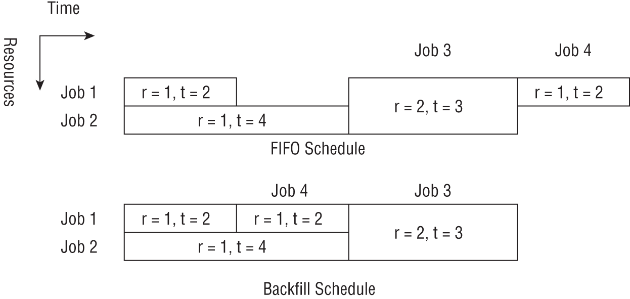
Figure 3-13: Backfill scheduling and FIFO scheduling
Summary
We discussed the various resources that are available for executing data-intensive applications and how they are managed in cluster environments. Depending on the frameworks, there can be many configuration parameters available to fine-tune the resources to map application requirements. Programming and deploying data analytics applications while being aware of the computing resources can greatly increase efficiency and reduce cost.
References
- 1. D. Merkel, “Docker: lightweight linux containers for consistent development and deployment,” Linux journal, vol. 2014, no. 239, p. 2, 2014.
- 2. A. B. Yoo, M. A. Jette, and M. Grondona, “Slurm: Simple linux utility for resource management,” in Workshop on job scheduling strategies for parallel processing, 2003: Springer, pp. 44-60.
- 3. J. V. Gautam, H. B. Prajapati, V. K. Dabhi, and S. Chaudhary, “A survey on job scheduling algorithms in big data processing,” in 2015 IEEE International Conference on Electrical, Computer and Communication Technologies (ICECCT), 2015: IEEE, pp. 1-11.
- 4. J. Krallmann, U. Schwiegelshohn, and R. Yahyapour, “On the design and evaluation of job scheduling algorithms,” in Workshop on Job Scheduling Strategies for Parallel Processing, 1999: Springer, pp. 17-42.
- 5. J. A. Pascual, J. A. Lozano, and J. Miguel-Alonso, “Analyzing the performance of allocation strategies based on space-filling curves,” in Job Scheduling Strategies for Parallel Processing, 2015: Springer, pp. 232-251.
- 6. A. K. Wong and A. M. Goscinski, “Evaluating the easy-backfill job scheduling of static workloads on clusters,” in 2007 IEEE International Conference on Cluster Computing, 2007: IEEE, pp. 64-73.
Notes
- 1
https://kubernetes.io/ - 2
https://slurm.schedmd.com/documentation.html - 3
https://hadoop.apache.org/docs/current/hadoop-yarn/hadoop-yarn-site/YARN.html - 4
https://www.switch.com/tahoe-reno/ - 5
http://worldstopdatacenters.com/4-range-international-information-hub/ - 6
https://www.switch.com/las-vegas/ - 7
https://www.digitalrealty.com/data-centers/northern-virginia - 8
https://www.fujitsu.com/global/about/innovation/fugaku/ - 9
https://www.olcf.ornl.gov/summit/ - 10
https://hpc.llnl.gov/hardware/platforms/sierra