CHAPTER 2
Data and Storage
Modern computing is a data-driven undertaking, with global enterprises accumulating petabytes of data that need to be stored and queried to extract valuable knowledge. Before the advent of big data technologies, we used file systems or relational databases for this purpose, but with datasets now in the petabytes scale and beyond, relational database management systems and traditional file systems cannot scale. Distributed file systems, NoSQL databases, and object storage systems are used today to handle these large datasets.
In this chapter, we will go through important concepts for data and storage. Since the main focus of this book is on data processing, we will keep our discussion limited to cover the most important topics.
Storage Systems
Storage systems are the platforms on which modern enterprises are built. They contain petabytes of data serving applications running nonstop. We have seen many types of storage systems over the years developed to support specific use cases and the demands of various applications. Because of this, we must consider many factors when choosing storage systems. In the era of large data, the first factor we need to take into account is how much data we are going to handle along with cost versus performance considerations.
There are numerous storage media available, including tape drives, hard disks, solid-state drives (SSDs), and nonvolatile media (NVM). Hard disks can be in disk arrays in RAID configurations to provide fault tolerance and increased I/O performance. A hard drive in our laptop is a block storage device that stores data in blocks of 512 bytes. As users, we never see the blocks because we access it through a file system created on top of the hard drive. The file system abstracts the block storage and provides a uniform API to facilitate data retrieval.
Furthermore, the type of access pattern we use for our data plays an important role. We may need to access data all at once, sequentially, randomly, or in a streaming fashion part by part. Also, we need to consider the type of data we store such as binary files (video, photos), text files, and whether we need to update the data after storage. Another aspect of a storage system is choosing between local and network storage. Local storage is attached to a computer, while in network storage the data can be in another computer that we access through the network. It all comes down to whether we need to share data among applications and users.
Storage for Distributed Systems
A computer cluster can be configured to access storage using three different methods. They are direct-attached storage (DAS), network-attached storage (NAS), and storage area networks (SAN). Figure 2-1 shows how these different storage systems are attached to a computing cluster.

Figure 2-1: Three ways to connect storage to computer clusters: direct-attached storage (left), network-attached storage (middle), storage area networks (right).
Direct-Attached Storage
Direct-attached storage is where a disk is attached to a computer directly. A laptop hard drive is a DAS storage. There are many protocols and hardware needed to attach disks to a computer, such as SATA, eSATA, NVMe, SCSI, SAS, USB, USB 3.0, and IEEE 1394.
If the server holding direct-attached storage goes down, that storage is no longer accessible to the other nodes. To avoid this problem, network-attached storage systems were developed. In NAS, multiple storage servers are connected to the compute servers using the regular network. Since NAS systems use a regular network, the data movement can create a bottleneck. As a result, storage-attached networks were developed with separate network access.
Hadoop File System (HDFS) is a distributed file system specifically designed to run on servers with direct-attached storage. In-house big data systems still find direct-attached storage-based clusters the most cost-effective solution for handling large amounts of data.
Storage Area Network
Instead of managing hard drives in each machine, we can put them in a central server and attach them to multiple computers through the network as block devices. In this mode, the individual machines will see storage as block storage devices, but how they are matched to the actual hard drives can be hidden. This method of attaching block storage through the network is called storage area network (SAN).
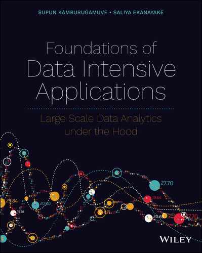
SAN uses dedicated networks from the storage to the compute nodes to provide high-speed access. The storage space is seen by the host as a block device. We can create a file system and store data here similar to a local hard drive. SAN storage servers come with sophisticated options that allow automatic replication and failure recovery. They can use disk arrays to speed up the I/O speeds. A SAN can be divided into the host layer, fabric layer, and storage layer, as shown in Figure 2-2.
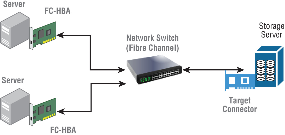
Figure 2-2: SAN system with a Fibre Channel network
- Host layer—The host layer resides in the servers that use the SAN storage. These servers are equipped with network devices called host bus adapters that connect the server to the SAN.
- Fabric layer—The fabric layer is responsible for bringing data from a host (initiator) to a target such as a port on a storage server. The fabric layer consists of network devices such as switches, routers, protocol bridges, gateway devices, and cables. There are many methods available to transfer data from host layer to storage layer, and while some of these are specific to SANs, sometimes they can use generally available networks as well. Depending on the network interfaces there are several protocols available to transfer the data between host and storage. Table 2-1 lists the different network channels and the protocols available.
Table 2-1: Storage Area Network Channels and Protocols
CHANNEL PROTOCOLS SPEED Fibre Channel Fibre Channel Protocol, NVMe-oF 32 Gbps InfiniBand iSER, NVME-oF, SRP 100 Gbps Ethernet iSER, NVME-oF, iSCSI 100 Gbps - Storage layer—The storage layer consists of the servers that host the storage devices of the SAN. Usually, many disks are combined in RAID configurations to provide both redundancies and high throughput. A SAN can have many types of storage systems in it such as NVMs, tape storage, and hard disk drive storage.
Network-Attached Storage
Compared to SAN, with network-attached storage [1] the user sees the remote storage as a mounted file system rather than a block device. NAS uses regular network hardware to connect to the storage servers. Network File System (NFS) and Server Message Block (SMB) are two of the protocols made to access files over the network. NAS is common in clusters to create a file system that can be used to share files among nodes and users.
DAS or SAN or NAS?
The advantages of DAS-based file systems are that we do not need to get separate storage servers and separate networking. Also, when the data required by computations is local to the machine, they work extremely fast compared to a NAS or SAN.
A cluster may consist of any combination of DAS, NAS, or SAN storage. For example, it can be configured with local hard disks and a NAS for sharing data among users. Another option could be a DAS/NAS/SAN hybrid where SAN is used to host the data for a relational database management system (RDBMS). Compared to NAS, SAN solutions provide high-bandwidth and low-latency access, but they are usually expensive as opposed to having local hard disks in machines or NAS systems. But the lines between NAS and SAN can be blurred due to various hardware options available. For instance, NAS can run on high-speed networks that are equal to a network you might see in a SAN system.
Storage Abstractions
Depending on the requirements, servers can access the storage using a block abstraction, a file system, or as objects (Figure 2-3). Usually, file systems are created on top of block storage, and object storage can use a file system or block storage to access the data.

Figure 2-3: Storage abstractions: block storage (left), file storage (middle), object storage (right)
Block Storage
This manner of storage saves data blocks. A block storage can place the data blocks into different hard drives. Depending on the abstractions, the user may not notice where they are physically present. Block storage is normally associated with SAN and DAS systems. On-premises clusters use SAN technologies to create block devices in the compute nodes or use directly attached hard drives. Directly using the block storage is done only in special applications that require the best performance possible.
Block storage is popular in cloud environments for hosting persistent data from virtual machines. Without persistent storage, a virtual machine would lose all its work when it is terminated. In clouds, technologies such as SAN used by block storage are not visible to the users. Here are some examples of block storage services in cloud environments:
- AWS Elastic Block Storage (EBS)1—EBS is raw storage exposed as a block device to virtual machines. We can create these devices with personalized configurations (size, etc.) and attach them to EC2 instances, or even create a file system on the attached storage device and use it from the EC2 instances to store data.
- Azure Disk Storage2—The same as EBS, premium storage is low-latency disk support for I/O intensive workloads in Azure virtual machines.
- Google Persistent Disks3—As with other services, Google Persistent disks provide a network-attached block storage for virtual machine instances.
File Systems
File systems are by far the most popular abstraction for storing data. There are hundreds of file systems available that work inside a single machine, across many machines, or even between machines in different data centers. A file system gives a file abstraction to store the data. The data is organized into hierarchical folders and stored in files that are addressed using a path name, which is a hierarchical designation consisting of the folders and the name of the file. File APIs are associated with the POSIX standard, which defines functions for basic file operations such as creating, opening, closing, reading, updating, and writing. POSIX standard allows different file systems to use similar APIs to access files, making it easier to create portable applications. An application can access a file as a stream of bytes, blocks, or set of structures.
A file system is divided into logical, virtual, and physical layers.
- Physical layer—This layer provides access to specific storage media such as hard disk and tape.
- Virtual layer—At this level, different file systems are developed to organize and manage the data in the physical layer. There are many file systems including EXT4, NTFS, etc.
- Logical layer—Many virtual file systems can be combined in a single file system view (root) to give access to files.
We are all familiar with the file systems at work in our local machines allowing access to the internal hard drives of the computer. A file system can be created on top of storage devices residing in a networked set of machines. NAS systems expose files through the network.
In cloud environments, there are virtual file systems that can be attached to virtual machines. Here are some of the file services available:
Object Storage
Object storage [2] stores data in a flat structure compared to the hierarchical structure in file storage. Object storage is used for storing large amounts of unstructured data such as text files, audio files, sensor data, and video files. These data do not have any structure associated with them to put them in places such as databases. Object storage has become the standard for keeping backups and archiving the data. Thanks to their flat structure, they can scale to store petabytes of data, and compared to file storage, they are easy to manage at that scale.
The storage unit in an object storage is called an object. An object stores the actual data along with metadata and has a unique identifier in the form of a URL or a text string. Object storage allows a rich set of metadata to be associated with the objects, and this information can be used for searching. There is no hierarchical structure in object storage systems such as folders as seen in file systems because everything is in a flat structure.
Clients typically use an HTTP-based RESTful API to access the objects. A RESTful API has methods such as PUT, POST, GET, and DELETE. The API uses the PUT and POST methods to create new objects, GET to retrieve them, and DELETE to delete objects. Usually, clients are provided to hide some of these details. RESTful APIs allow object stores to be accessed from anywhere with an internet connection such as a mobile device. Object storage is usually categorized as write once read many (WORM) storage as they do not allow updates to the existing objects.
Object storage is common in public and private clouds. There are object stores that can be deployed in in-house clusters as well. For the user, it is not obvious how the objects are stored on the disks. Object storage can use file systems or block storage to house data.
Data Formats
We encounter data in many different formats. Some common examples are CSV, JSON, XML, Text, and Binary types. Every format has a defined storage structure. CSV, JSON, and XML are all text-based formats. They define the structure using other text elements. For example, in a CSV file, the attributes are separated by a marker such as a comma. Most data formats have some mechanism to define a schema. Schemas provide a mechanism to understand a document.
JSON and XML are two of the most popular data formats used for transferring data among distributed systems like web-based services and clients. Text formats take more space to store and more processing power to parse but are easier to work with because they can be inspected by regular text editing tools. For larger files that require more compact and efficient storage mechanisms with the ability to search faster, there are binary file formats such as Parquet and Avro.
XML
XML stands for Extensible Markup Language. It has a hierarchical format for storing data. XML documents contain elements, attributes, and values. An element can contain other elements as well as attributes. The following is a simple XML document. In this example, the top element is called
message
and is enclosed in <>. Every element has an ending tag with the syntax </>. The header element has an attribute called
contentType
.
<message><header contentType='text'><to>serviceX</to><from>clientY</from></header><body>Hello from client</body></message>
XML can optionally have a schema attached to a document. The schema specifies the structure of the document and constraints on the data. For instance, it can specify that the document has a
message
element with two elements called
header
and
body
one after another (in order). Furthermore, it can specify constraints such as how a name cannot contain special characters. If a document is presented with only one element inside the message element, we can reject it as an invalid document according to the schema. Here is the corresponding schema for the previous XML document:
<xs:schema attributeFormDefault="unqualified" elementFormDefault="qualified" xmlns:xs="http://www.w3.org/2001/XMLSchema"><xs:element name="message"><xs:complexType><xs:sequence><xs:element name="header"><xs:complexType><xs:sequence><xs:element type="xs:string" name="to"/><xs:element type="xs:string" name="from"/></xs:sequence><xs:attribute type="xs:string" name="contentType"/></xs:complexType></xs:element><xs:element type="xs:string" name="body"/></xs:sequence></xs:complexType></xs:element></xs:schema>
XML was the dominant method of data transfer in the early days of web-based services. Many companies joined together to create a set of specifications around XML to shuttle data between services and client programs. SOAP [3] and WSDL [4] were some of the standards created around XML with this initiative. SOAP defines a message format with a header and a body for encapsulating a network message. WSDL is a specification to describe a service along with the request and response formats of the messages. These standards allowed any framework to read messages originating from a client as long as they adhered to the standard specifications. There are many other standards such as Extensible Stylesheet Language Transformations (XSLT) [5] for specifying transformations on XML data and XPath [6] for addressing parts of XML documents.
XML parsing is a relatively time/resource-consuming task because of its verbosity as well as the constraint enforcement. As a result, it requires more space to store it, and people have moved away from XML to a much simpler JSON format that is easier for machines to parse and humans to understand.
JSON
JavaScript Object Notation (JSON) is the most popular data format used in web services. Compared to XML, JSON is less verbose, but some can argue it is still complicated. JSON is used mostly with REST services on the web, which is the dominant form of defining services. A JSON document has two main structures. The first is a collection of name-value pairs, and the second is an ordered list of values. The following is a JSON document for the same XML message we described earlier. Note that the root message element is no longer needed, and the end tag is simplified to a closing bracket.
header
is an object that has a set of key-value pairs.
body
has only one value.
{"header": {"@contentType": "","to": "serviceX","from": "clientY"},"body": "Hello from client"}
In most cases, the raw data coming from a user or an application will be in JSON or XML format. These data formats are not designed to be queried at large scale. Imagine having a large number of JSON objects saved in the file system. To get useful information, we would need to parse these files, which is not as efficient as going through a binary file.
CSV
Comma-separated values (CSV) is a text file format for storing tabular data. A table is a set of rows with columns representing individual attributes of rows. In a CSV file, each data row has a separate line. For every row, the values of columns are separated by a comma. Values are stored as plain text. The following is a comma-separated CSV file that shows the grades of students for different subjects they have taken. There is a header in the CSV file to label each column in the table.
"Name", "Subject-1", "Subject-2", "Subject-3", "Subject-4""Joshua Johnson", A+, B+, A, B-"Harry Wilson", A+, A+, A, B"Gerty Gramma", A+, A+, A, A-"Android Electric", A-, B+, C+, B+
CSV is a popular data format for storing small to medium-scale data. Popular spreadsheet tools all support the loading and saving of CSV files as tabular data. Even though everyone is using CSV files, it is not a full standard. Different implementations can choose a host of methods to handle edge cases.
As an example, since CSV files are comma separated, a comma inside an attribute value needs to be handled independently. An implementation can choose to wrap values in quotation marks to handle commas inside a value. The same is true for line breaks within values. Some CSV implementations support escape characters to handle such cases as well. Other separators such as tabs, spaces, and semicolons are used in CSV files to separate the attributes. There is a specification called RFC4180 developed to standardize CSVs, but in practice, it is not 100 percent followed by the tools.
Since CSV is a text representation, it can take up a large amount of space compared to a compact binary format for the same data. We can have a CSV file with two integer columns to make our point. Assume our row has the following two integers:
7428902344, 18234523
To write that row as plain text, we need to translate each character into a character encoding value. If we assume ASCII format and allocate 1 byte for each character, our row will require 21 bytes (for each digit, line end character, delimiter, and space). By using a binary format, we need only 8 bytes to write the integer values, a reduction of more than half. Additionally, we cannot look up a value in a CSV file without going through the previous lines since everything is text. In a structured binary file, the lookups can be much more efficient. Nevertheless, CSV files are widely used because humans can read them and the rich set of tools available to generate, load, visualize, and analyze CSV files.
Apache Parquet
We can break up a table of data by storing the rows and columns in contiguous spaces. When storing rows, we refer to it as row-wise storage, and when storing columns, we call it column-wise storage or columnar storage. Parquet stores the data in the columnar format. It is a binary storage file format for tabular data. Let's take a look at a simple example to understand the columnar option.
Assume we have a table with two columns and five rows of data. The first column is holding a 32-bit integer value, and the second column has a 64-bit integer value.
First, Second10, 12304566323, 12304326521, 14566366322, 12306366212, 123046362
In the case of CSV, we store this file as a plain text file. For binary we need to decide in what order we are going to store the data. Assume we choose row-wise. Figure 2-4 illustrates how this would look. Each row has 12 bytes with a 4-byte integer and an 8-byte integer. The values of each row are stored contiguously.

Figure 2-4: Storing values of a row in consecutive memory spaces
We can store the values of columns contiguously as well. Figure 2-5 shows the bytes when storing in this format.

Figure 2-5: Storing values of a column in consecutive memory spaces
Both formats have their advantages and disadvantages depending on the access patterns and data manipulation requirements of the applications. For example, if an application needs to filter values based on those contained in a single column, column-based representation can be more efficient because we need to traverse only one column stored sequentially in the disk. On the other hand, if we are looking to read all the values of each row consecutively, row-based representation would be preferable. In practice, we are going to use multiple operations of which some can be efficient with row-wise storage and others with column-wise storage. Because of this, data storage systems often choose one format and stick to it while others provide options to switch between formats.
Parquet6 supports the following data types. Since it handles variable-length binary data, user-defined data can be stored as binary objects.
- Boolean (1 bit)
- 32-bit signed integer
- 64-bit signed integer
- 96-bit signed integer
- IEEE 32-bit floating-point values
- IEEE 64-bit floating-point values
- Variable-length byte arrays
As shown in Figure 2-6, a Parquet file contains a header, a data block, and a footer. The header has a magic number to mark the file as parquet. The footer contains metadata about the information stored in the file. The data block forms the actual data encoded in a binary format.
The data blocks are organized into a hierarchical structure with the topmost being a set of row groups. A row group contains data from a set of adjacent rows. Each group is divided into column chunks for every column in the table. A column chunk is further divided into pages, which is a logical unit of saving column data.
The footer contains metadata about the data as well as the file structure. Each row group has metadata associated with it in the form of column metadata. If a table has N columns, there is N number of metadata inside the row group per column chunk. The column metadata contains information about the data types and pointers to the pages.
Since the metadata is written at the end, it allows Parquet to write the files with a single pass. This is possible because we can write the data without needing to calculate the structure of the data section. For example, Parquet does not need to calculate the boundaries of the data before having it written to the disk. Instead, it can calculate this information while writing the data and include the metadata at the end in the footer. As a result, metadata can be read at the end of the file with a minimal number of disk seeks.

Figure 2-6: Parquet file structure
Apache Avro
Apache Avro7 (or simply Avro) is a serialization library format that specifies how to pack data into byte buffers along with data definitions. Avro stores data in a row format compared to Parquet's columnar format. It has a schema to define the data types. Avro uses JSON objects to store the data definitions in a user-friendly format and binary format for the data. It supports the following data types similar to Parquet:
- Null having no value
- 32-bit signed integer
- 64-bit signed integer
- IEEE 32-bit floating-point values
- IEEE 64-bit floating-point values
- Unicode character sequence
- Variable-length bytes
We can use the Avro schema to code generate objects for easy manipulation of our data. It has the option to work without code generation as well. Let's look at the Avro schema.
Avro Data Definitions (Schema)
Here we can see a simple Avro schema to represent our message class:
{"name": "Message","type": "record","namespace": "org.foundations","fields": [{"name": "header","type": {"name": "header","type": "record","fields": [{"name": "@contentType","type": "string"},{"name": "to","type": "string"},{"name": "from","type": "string"}]}},{"name": "body","type": "string"}]}
We first set the name, type, and namespace of the object. Our object's fully qualified name would be
org.foundations.Message
. Then we specify the fields. We have a
header
field and a
body
field. The
header
field is another record with three fields. The
body
field is of type
string
.
Code Generation
Once we have the schema defined, we can generate code for our language of choice. The generated code allows us to easily work with our data objects. Code generation is excellent when we know the data types up front. This would be the approach for custom solutions with specific data types. If we want to write a generic system that allows users to define types at runtime, code generation is no longer possible. In a scenario like that, we rely on Avro without code generation.
Without Code Generation
We can use Avro parsers to build and serialize Avro objects without any code generation. This is important for applications with dynamic schemas that are only defined at runtime, which is the case for most data processing frameworks where a user defines the type of data at runtime.
Avro File
When serialized, an Avro file has the structure shown in Figure 2-7. It possesses a header with metadata about the data and a set of data blocks. The header includes the schema as a JSON object and the codec used for packing the values into the byte buffers. Finally, the header has a 16-byte sync marker to indicate the end. Each data block contains a set of rows. It has an object count and size of total bytes for the rows (objects). The serialized objects are held in a contiguous space followed by the 16-byte marker to indicate the end of the block. As with Parquet, Avro files are designed to work with block storage.
Schema Evolution
Data can change over time, and unstructured data is especially likely to change as time goes by. Schema evolution is the term used to describe a situation in which files are written using one schema, but then we change the schema and use the new one with the older files. Schema evolution is something we need to carefully plan and design. We cannot change the old schema arbitrarily and expect everything to work. Some rules and limitations define what changes are possible for Avro:
- We can add a new field with a default value.
- We can remove a field with a default value.
- We can change, add, or remove the
docattribute.
Figure 2-7: Avro file structure
- We can change, add, or remove the
orderattribute. - We can change the default value for a field.
- We can change a nonunion type to a union that contains only the original type.
To change the schema like this, we need to define our original schema fields susceptible to change with the previous modification rules. For example, we must set default values if we are hoping to change a field.
Protocol Buffers, Flat Buffers, and Thrift
Protocol buffers,8 Flat buffers,9 and Thrift10 are all language-independent, platform-neutral binary protocols for serializing data. Users of these technologies must define a schema file with the data structure of the objects they need. All these technologies have a compiler that generates source code in the programming language of choice to represent the objects defined.
We can use these as regular objects in our code. Once it becomes necessary to save or transfer them through the network, we can convert the objects into binary formats. The schema is embedded directly into the code generation and enforced by the program at runtime.
Here we have a definition for our message object with protocol buffers. The other formats all follow the same process.
message "header" {message HEADER {required string @contentType = 0required string to = 1required string from = 2}required HEADER header = 0required string body = 1}
In the previous code snippet, we define a protocol buffer message with several fields. The next step is to generate a set of source files with our programming language of choice from these definitions. Once the files are generated, we use them in our program as regular objects. We can create our object, set values to it, and read values from it.
Data Replication
Replication is a technique used for keeping copies of the same data in multiple computers. We call a copy of the data in a computer a replica. We use replication to achieve the following:
- Fault tolerance—If one replica is not available, systems can continue to process requests from the other replicas.
- Increased performance—We can keep replicas in multiple regions as well as multiple computers within a single cluster. By staying close to the computers that access it, data can be served faster.
- Scaling—When data is in multiple computers, it can be simultaneously accessed by many users.
Keeping replicas is not as simple as copying data to multiple computers. If we have static data that does not change after the initial write, all we need to do is copy them to multiple computers at the initial write. We call such data unimmutable data. Some systems support this model, the most notable of which is the Hadoop File System. Even in these systems, the data needs to be rebalanced in case there is more load on one computer or when nodes fail. If we allow data to be modified, we will need to keep the replicas consistent when updates occur.
On the surface, it seems if a writer of a dataset takes ![]() time units, it will require
time units, it will require ![]() time for replicating the data to three machines. Replicating the data can be done in a pipelined way that reduces this time drastically. This is shown in Figure 2-8 where a client usually sends data in some form of data chunks (streams), which can be pipelined through the replicas along with acknowledgments.
time for replicating the data to three machines. Replicating the data can be done in a pipelined way that reduces this time drastically. This is shown in Figure 2-8 where a client usually sends data in some form of data chunks (streams), which can be pipelined through the replicas along with acknowledgments.
A system can choose synchronous or asynchronous replication. It can also be designed as a single leader replication or multileader replication system. We may create a system with any of these combinations.
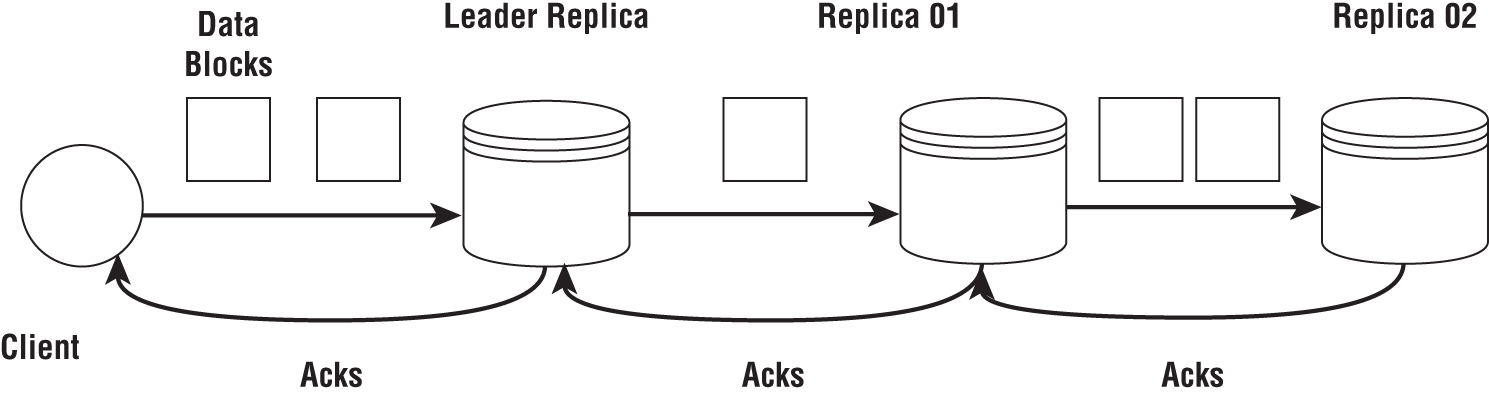
Figure 2-8: Pipelined replication
Synchronous and Asynchronous Replication
In synchronous (eager) replication systems, the system makes sure the replication is complete before sending a response back to the client for a write request. This means the client needs to wait until the replication is done, which can take time. For asynchronous replication systems, the server can immediately respond after the update is applied to the leader replica. With asynchronous replication, if an error occurs during replication, the client has no way of knowing whether its write has failed. Asynchronous replication is fast compared to synchronous, and with asynchronous replication, clients might see stale data when some replicas are not updated in time.
Single-Leader and Multileader Replication
In single-leader replication systems, the updates are controlled by a lone server acting as the leader. The replicas are called followers. Clients always connect to the leader to update the data. A client sends a request to update the data to the leader that in turn updates its copy. Now the leader needs to update the followers. A single leader may act as a bottleneck for handling large workloads, and if the data store expands across multiple data centers, single-leader replication systems will not scale.
As the name suggests, multileader systems can have multiple leaders at the same time. They permit simultaneous updating of the replicas. Allowing multiple clients to update different replicas is a complex process that requires careful coordination between the leaders. It can take a significant amount of resources and slows down the systems in general. Because of this, multileader replication is mostly used in systems that expand across multiple data centers. Replicating data across data centers in separate regions is a widespread practice for serving far-flung users.
If data is replicated in machines close to each other, a network failure or a power failure can make the data inaccessible, defeating one purpose of replication. To avoid such situations, data can be replicated in a way that reduces the probability of failures. For example, it can be replicated in multiple data centers.
Data Locality
Data locality comes from the general principle of the owner-computes rule in parallel computing. The owner-computes rule states that when a data partition is assigned to a computer, that computer is responsible for all the computations associated with the partition.
For a computer to work on a data partition, we need to load the data into the main memory of that computer. But what happens if the data is in another computer accessible only through the network? We would have to move that data through the network to the relevant computer. At the dawn of the big data revolution, network speeds were limited, and moving large amounts of data between computers was a time-consuming operation. It was much easier to move the computations to the computers with the data that they were going to operate for the sake of performance. This process of trying to reduce data movement is called preserving the data locality.
Data locality can come in many levels. The best-case scenario is that relevant data required by every task is in the computer that it runs on, thus having no need to move data through the network. But in practice this is harder to achieve. If the data is not in the same computer, it is better to at least store it in the same server rack where network speeds are faster.
Hard disk speeds have not increased as much as network speeds over the past decade. Current networks can send data much faster. Because of this, the value of data locality is greatly reduced in modern clusters. Furthermore, preserving data locality in a cluster shared with multiple applications is hard. Cloud-based object storage services that provide data as a service have further reduced the importance of data locality. Nevertheless, if conditions permit, preserving data locality can reduce the data read time significantly for applications.
Disadvantages of Replication
Even though replication has many advantages and is often used in distributed systems, it does come with some caveats.
- Additional disk space—Replicating data requires additional disk capacity. To add capacity, not only do we need more disks, we have to acquire additional computers and network bandwidth and extend the cluster to host the disks. Also, when more and more nodes are added to a cluster, distributed operations that span more nodes can become slow due to network communication overhead.
- Updates are slow—Multiple replicas need to be kept up-to-date. When an update happens to data, that update replication process can take considerable time depending on the type of replication chosen.
Data Partitioning
Imagine a large data collection we intend to process using multiple computers. We must first divide the data among computers so that they can work on part of the dataset. Data partitioning is the process of distributing data among multiple computers so that different computers/processes can act on them separately but simultaneously. When we consider data processing, partitioning comes under the broad umbrella of load balancing. Load balancing is always a hard problem to tackle in distributed computing.
Reasons for partitioning data include the following:
- Scalability—The data is distributed among many computers, allowing larger data sizes that do not fit into one machine to be processed in parallel.
- Performance—The data can be processed in parallel using multiple computers, reducing the overall compute time and increasing the amount of data processed per unit.
- Provide operational flexibility—Data can be partitioned according to different needs of the applications. One example is to partition data according to how old they are. New data can be given more priority in both processing and storage, while old data can be stored using cheaper methods.
- Availability—When data is present in multiple computers, even if part of a machine goes down, other parts of the data can be still available.
Depending on the data abstraction like a table or an array, different data partitioning techniques can be used. Because most data are stored as tables, let's look at horizontal, vertical, and functional partitioning methods for table data. We will use Table 2-2 as an example.
Table 2-2: Original Dataset with Four Rows
| ID | DATE | CONTENT | URL | AUTHOR |
|---|---|---|---|---|
| 984245 | 2020-01-13 | {json content} | http:://jsonc.io/one | Ted Dunken |
| 245213 | 2019-11-02 | {json content} | AB Foundation | |
| 532134 | 2019-12-05 | {json content} | http:://jsonc.io/now | Nethan Salem |
| 556212 | 2020-02-09 | {json content} | http:://jsonc.io/oxy |
Vertical Partitioning
Vertical partitioning divides the data table vertically into different sets of columns and stores them separately. Tables 2-3 and 2-4 show a vertical partitioning of our table where we included the first three columns in one table and the first column along with the last two columns in another.
Table 2-3: First Table with Only First Three Columns of Original Table
| ID | DATE | CONTENT |
|---|---|---|
| 984245 | 2020-01-13 | {json content} |
| 245213 | 2019-11-02 | {json content} |
| 532134 | 2019-12-05 | {json content} |
| 556212 | 2020-02-09 | {json content} |
Table 2-4: Second Table With The First Column and the Last Two Columns from the Original Table
| ID | URL | AUTHOR |
|---|---|---|
| 984245 | http:://jsonc.io/one | Ted Dunken |
| 245213 | AB Foundation | |
| 532134 | http:://jsonc.io/now | Nathan Salem |
| 556212 | http:://jsonc.io/oxy |
Vertical partitioning can help to isolate data attributes that are used infrequently in queries from the ones that are used frequently.
Horizontal Partitioning (Sharding)
Horizontal partitioning (also known as sharding) is used extensively for partitioning data. Here we partition by the rows of the table. Tables 2-5 and 2-6 show how the data is partitioned according to the year.
Table 2-5: Horizontal Partition with the Year 2019
| ID | DATE | CONTENT | URL | AUTHOR |
|---|---|---|---|---|
| 245213 | 2019-11-02 | {json content} | AB Foundation | |
| 532134 | 2019-12-05 | {json content} | http:://jsonc.io/now | Nathan Salem |
Table 2-6: Horizontal Partition with the Year 2020
| ID | DATE | CONTENT | URL | AUTHOR |
|---|---|---|---|---|
| 984245 | 2020-01-13 | {json content} | http:://jsonc.io/one | Ted Dunken |
| 556212 | 2020-02-09 | {json content} | http:://jsonc.io/oxy |
The attribute or set of attributes used for partitioning the data is called the partitioning key. There are many strategies available in this respect. According to the requirements of the applications, we can choose from various partitioning schemes, and we describe a few here:
- Hash partitioning—Done by applying a hash function to the partitioning key. The simplest hash partitioning mechanism is to get the hash and then use the modules of the number of partitions. However, this method can produce imbalanced partitions for most practical datasets.
- Range partitioning—If a record is within a range, it is assigned to the partition for that range. For instance, in our previous example, we partitioned the data according to the date attribute. If we are using a numerical key for partitioning, it can be based on numerical ranges.
- List partitioning—This keeps a list of values for each partition. If an attribute has a value that belongs to a list, it is assigned to the corresponding partition. For example, if a city belongs to the list of cities in a country, the record is assigned to a partition for that country.
- Composite partitioning—We can use a combination of the previous strategies. We might first partition the data according to range partitioning, and within those partitions we use list partitioning to separate the data further. The same key or different keys can be used for composite partitioning.
- Round-robin partitioning—Consecutive records are assigned to consecutive partitions in a round-robin manner. This is one of the easiest ways to partition the data as no consideration is given to the data properties.
Hybrid Partitioning
Both vertical and horizontal partitioning are used on the same dataset. As such, we can partition data horizontally according to the year and vertically to separate the content column. This is shown in Tables.
Table 2-7: First Horizontal Partition of 2019
| ID | DATE | URL | AUTHOR |
|---|---|---|---|
| 245213 | 2019-11-02 | AB Foundation | |
| 532134 | 2019-12-05 | http:://jsonc.io/now | Nathan Salem |
Table 2-8: Second Horizontal Partition of 2020
| ID | DATE | URL | AUTHOR |
|---|---|---|---|
| 556212 | 2020-02-09 | http:://jsonc.io/oxy | |
| 984245 | 2020-01-13 | http:://jsonc.io/one | Ted Dunken |
Table 2-9: First Vertical Partition
| ID | CONTENT |
|---|---|
| 245213 | {json content} |
| 532134 | {json content} |
Table 2-10: Second Vertical Partition
| ID | CONTENT |
|---|---|
| 556212 | {json content} |
| 984245 | {json content} |
Considerations for Partitioning
When multiple computers work on a single problem, it is important to assign an equal amount of work to each machine. This process is called load balancing. It is a concept applied to many distributed systems including services, data analytics, simulations, etc. Load balancing is especially important when multiple computers execute tasks in parallel.
In distributed data processing systems, one significant concern about data partitioning is how to distribute the data equally among machines. Without balanced partitioning, valuable computing resources can be wasted, and applications may take longer than necessary to complete. Load balancing the partitions is tied to both data and the algorithms used.
The following is a hypothetical example of four processes doing the same computation in parallel. Say we have a large dataset filled with numbers, and we are going to multiply individual elements of this dataset by a number and get the sum. Unfortunately, we did not divide the dataset equally among the four processes, and instead assigned 50 percent, 15 percent, 15 percent, and 20 percent to four processes. Assume it takes time t to process 1 percent of the dataset. As we can see, the work is not load-balanced across the four processes. The processes take 50t, 15t, 15t, and 20t time to complete. Since they are running in parallel, the application takes the slowest process's time to complete; in our example, it is 50t. Now assume we instead divided the work equally among the processes, 25 percent apiece. In this case, each process will take 25t time to complete, a two times speedup over the previous work assignment.
For data applications, load balancing is closely associated with partitioning. Parallel processes in data processing systems work on partitions of the data. So, it is important to keep the data partitions roughly the same size.
NoSQL Databases
NoSQL database is a broad term used to identify any data storage that is not a relational database. Some NoSQL databases support SQL queries, so the term should not be confused with SQL. Even though there were databases not designed according to the ACID principles of RDBMS from the very early days of computing, NoSQL databases became mainstream with the big data movement starting in the early 2000s. NoSQL databases [7] are all developed to optimally store and query data with specific structures. Some are designed to scale to petabytes of storage, while others support specific data types in a much smaller scale.
Data Models
We can classify NoSQL data stores according to the data models they support. There are key-value databases, document databases, wide column databases, and graph databases.
Key-Value Databases
These databases store key and value pairs with unique keys. The model is quite simple and can store any type of data. They also support create, read, update, and delete (CRUD) operations and are referred to as schema-less. The datastore does not know about the data it has, and it is only available to the application. As a result, these data stores cannot support complex queries that require knowledge of the structure of the data stored. Nevertheless, many data problems fit into these data stores owing to their simplicity. Table 2-11 shows a sample data store with few key value pairs.
Table 2-11: Key Value Data Store
| KEY | VALUE |
|---|---|
| K1 | Data bases |
| K2 | <t>data</t> |
| K3 | {a: “1”, k: “2”} |
Document Databases
A document database stores data using semistructured formats like JSON documents. They can be thought of as key-value stores with a semistructured value. Since the data store has knowledge about the structure of the values, it can support complex queries. For example, we can query these databases with an internal attribute of a JSON object, which is not possible in a key-value database. Table 2-12 shows the data store for a document database with a JSON document.
Table 2-12: Document Store
| KEY | VALUE (JSON DOCUMENT) |
|---|---|
| K1 | { "header": { "@contentType": "", "to": "serviceX", "from": "clientY" }, "body": "First message" } |
| K2 | { "header": { "@contentType": "", "to": "serviceX", "from": "clientY" }, "body": "Second message" } |
Wide Column Databases
Wide column databases [8] have table-like structures with many rows each possessing multiple columns. Wide column databases should not simply be thought of as RDBMS tables with a lot of columns. Instead, they are more similar to multilevel maps, as shown in Table 2-13. The first level of the map is the key that identifies the row. The columns are grouped into column families. A column family can have many columns and is identified by a column key (which can be dynamic). Since columns are dynamic, different rows may have a different number of columns.
Graph Databases
Graph databases are designed to represent and query graph structures efficiently and in an intuitive way. We can use relational databases, document databases, and key-value databases to store graph data. But the queries as implemented on these databases are more complex. To simplify the queries to be more suitable for graph data, different query languages are used. Some popular query languages include Gremlin [10] and Cypher [9]. At the present time there is no standard query language such as SQL available for graph databases. A graph database can use a table structure, a key-value structure, or a document database to actually store the data.
Table 2-13: Wide Column Store
| KEY | FIRST COLUMN FAMILY | SECOND COLUMN FAMILY | |||
|---|---|---|---|---|---|
| COLUMN KEY1 | COLUMN KEY2 | COLUMN KEY3 | COLUMN KEY 4 | COLUMN KEY 5 | |
| K1 | -- | -- | -- | -- | -- |
| K2 | -- | -- | -- | -- | -- |
CAP Theorem
CAP is a broad theorem outlining a guiding principle for designing large-scale data stores. It specifies a relationship between three attributes of a distributed data store called consistency, availability, and partition tolerance [11]:
- Consistency—Every read request will give the latest data or an error.
- Availability—The system responds to any request without returning an error.
- Partition tolerance—The system continues to work even if there are network failures.
Large-scale data stores work with thousands of computers. If a network failure divides the nodes into two or more subsets without connectivity between those subsets, we call it a network partition. Network partitions are not common in production systems, but they still need a strategy when one occurs. The theorem states that a distributed data store needs to pick between consistency and availability amid a network partition. Note that the system must select between the two only when a failure happens. Otherwise, the data store can provide both consistency and availability to its data. The original goal of CAP theorem was to categorize data stores according to two attributes they support under failure, as shown in Figure 2-9.
Let's examine why a system needs to pick between availability and consistency. Should a network partition occur, the system is divided into two parts that have no way to communicate with each other. Say we choose to make the system available during the network partition. While the network partition is present, a request comes to update a data record that is fed into a machine in one side of the partition. We wanted to make the system available, so we are going to update the data. Then another request comes to a machine on the other side of the network partition to read the same data. This machine has a copy of the data, but it is not updated with the latest version because we could not propagate the update. Since the second partition does not know about the update, it will return an old data record to the client, which makes the system inconsistent. Now if we choose to make the system consistent, we will not return the data for the second request because we do not know whether the data is consistent, making our system in violation of the availability constraint.

Figure 2-9: CAP theorem
In practice, things are much more complicated than what the CAP theorem tries to capture, so CAP is more of a guiding principle than a theorem that clearly describes the capabilities of a system [12]. Some systems only have consistency guarantees in a network partition situation when operating under certain configurations. Most practical databases cannot provide either consistency or availability guarantees as stated in the theorem amidst failures. Furthermore, the CAP theorem is valid only under network partition scenarios, and there are many other failures possible in distributed systems. There is another theorem called PACELC [13] that tries to incorporate runtime characteristics of a data store under normal circumstances. The PACELC theorem states that under network partitions there is the consistency-availability trade-off, and under normal operation there is the latency-consistency trade-off.
Message Queuing
Message queuing is an integral part of data processing applications. Message queues are implemented in message broker software systems and are widely used in enterprises, as shown in Figure 2-10. A message broker sits between the data sources and applications that consume the data. A message source can be any number of things such as web users, monitoring applications, services, and devices. The applications that consume the data can again act as a data source for other applications. Because of this, message queuing middleware is considered the layer that glues together enterprise solutions. Message queuing is used in data processing architectures for the following reasons.
- Time-independent producers and consumers—Without message queues, the producing applications and consuming applications need to be online at the same time. With message queues in the middle, a consuming application may not be active when the sources start producing the data and vice versa.
- Act as a temporary buffer—Message queues provide a buffer to mitigate the temporal differences between message producing and message consuming rates. When there is a spike in message production, data can be temporally buffered at the message queue until the message rate drops down to normal. Also, when there is a slowdown in the message processors, messages can be queued at the broker.
- Transformation and routing—Messages are produced by a cloud of clients that make a connection to the data services hosted in a different place. The clients cannot directly talk to the data processing engines because different clients produce different data, and these have to be filtered and directed to the correct services. For such cases, brokers can act as message buses to filter the data and direct them to appropriate message processing applications.

Figure 2-10: Message brokers in enterprises
Message queuing systems provide many functions to integrate different systems. These functions depend on specific implementations, but there are some attributes common in all message brokers such as message durability and transactional processing, to name a few.
Figure 2-11 shows a message queue in its most simplified form. There is a single producer and a consumer for the message queue. All the messages produced are received in that order by the consumer. But in reality, the picture is more complicated. There can be multiple consumers and producers, and the queue can be replicated across multiple nodes.

Figure 2-11: Message queue
The producers push (send) messages to the queue. Consumers can be pulling messages from the queue, or it can be pushing messages to the consumer. This choice of push or pull at the consumer affects how many consumers a queue can have. If the queue is pushing to the consumer, there can be multiple consumers in a load balancing group. When the consumers are pulling messages, it is harder to have multiple consumers. This happens because consumers do not work in synchronization to get the messages from the queue.
Message Processing Guarantees
A message broker can provide delivery guarantees to its producers and consumers. These guarantees include the following:
- At least once delivery—Messages are never lost but can be processed multiple times.
- At most once delivery—Messages may get lost, but they will be delivered only one time at most.
- Exactly once delivery—Messages are delivered exactly once.
Delivery guarantees are closely related to the fault tolerance of the system. If a queuing system is not fault tolerant, it can provide only at most once delivery guarantees. To be fault-tolerant, the systems can replicate messages and save them to persistent storage. The producers connecting to the message queue need to adhere to a protocol that transfers the responsibility of the messages to the queuing system. Also, the consumers need a protocol to transfer the responsibility of the messages from the queue. It is extremely difficult to provide exactly-once delivery guarantees in message queues.
Durability of Messages
Message queuing systems can store the data until they are successfully processed. This allows the queuing systems to act as fault-resilient temporary storage for messages. By saving messages to the persistent storage, they can keep more messages than otherwise permitted on the main memory. If the messages are kept in the disk of a single server and it goes down, the only way to recover those messages is by restarting that node.
Another way to ensure the durability of the messages is to replicate them to multiple nodes running the brokers, as shown in Figure 2-12. If the replicas are saved to persisted storage, it provides robust durability for the messages. Replication comes at a cost here as message systems expect to provide low-latency operations.
Figure 2-12: Message queue replication
Acknowledgments
An acknowledgment is a response message that indicates the processing status of a message. Acknowledgments help the producers and consumers of the messages to safely transfer the message responsibility. We can send acknowledgments for every message or for several messages at once.
Producers can choose among a few options:
- Fire and forget—The producer does not receive an acknowledgment after it sends the message to the broker. The message may get lost at the broker. This method offers the best performance.
- With acknowledgments—A positive acknowledgement from the broker means the message has been safely accepted by the broker and the client is no longer responsible for the message. A negative acknowledgment means the broker could not accept the message.
Message consumers can also choose different types of acknowledgments to the broker:
- No acknowledgments—This offers at most once delivery to the consumers. The messages may get lost if errors such as network connection failures or consumer failures occur after the broker sends the message.
- Auto-acknowledgments—Messages are acknowledged without considering the processing at the consumer. If the message is acknowledged and the consumer fails before processing the message, it can lead to a lost message.
- Manual acknowledgments—Messages are acknowledged after they are processed by the consumer. If the consumer fails after processing the message but before it can send the acknowledgment, the message can be processed more than once at the consumer. Also, it can take an arbitrarily long time to process a message, and acknowledgments can be delayed.
Storage First Brokers and Transient Brokers
Message queues have been around for a long time, dating back to many years before the data revolution. These traditional message brokers were designed around transient messages where producers and consumers were online mostly at the same time and produced/consumed messages at an equal rate. Popular message brokers such as RabbitMQ11 and Apache ActiveMQ12 were all developed around this assumption. These brokers are neither designed to handle large amounts of data produced in a short period of time nor serve them to applications over a long period by storing them.
Owing to the large volumes of data involved in big data applications, storage first brokers were created. The first notable broker of this category was the Apache Kafka13 broker. These store data in the disk before they are delivered to the clients. They use techniques to divide the queues into partitions so that data can be distributed across nodes. Transient brokers and storage first brokers are suitable for different applications and environments. Situations in which storage first brokers are best suitable include the following:
- Large amounts of data are produced in a small time window in which the consumers cannot process this data.
- Consumers can be offline while large amounts of data are produced, leading to them being stored at the brokers.
- The data needs to be kept at the broker for longer periods to stream to different applications at separate times.
These are situations in which transient message brokers are best:
- Low-latency message transfer at the brokers.
- Dynamic routing rules at the message broker.
Both transient and storage first brokers are used in data processing systems depending on the use cases. But for handling large workloads, we would most likely need a storage first broker.
Summary
There is a vast amount of research and literature available in different databases, distributed file systems, and data formats. Data processing systems are tightly coupled to this data layer to read and write data. We discussed the low-level data storage systems, various data formats, NoSQL databases, and message brokers.
References
- 1. G. A. Gibson and R. Van Meter, “Network attached storage architecture,” Communications of the ACM, vol. 43, no. 11, pp. 37–45, 2000.
- 2. M. Factor, K. Meth, D. Naor, O. Rodeh, and J. Satran, “Object storage: The future building block for storage systems,” in 2005 IEEE International Symposium on Mass Storage Systems and Technology, 2005: IEEE, pp. 119–123.
- 3. D. Box et al., “Simple object access protocol (SOAP) 1.1,” ed, 2000.
- 4. E. Christensen, F. Curbera, G. Meredith, and S. Weerawarana, “Web services description language (WSDL) 1.1,” ed: Citeseer, 2001.
- 5. J. Clark, “Xsl transformations (xslt),” World Wide Web Consortium (W3C). URL
http://www.w3.org/TR/xslt, vol. 103, 1999. - 6. J. Clark and S. DeRose, “XML path language (XPath),” ed, 1999.
- 7. NOSQL Link Archive. “LIST OF NOSQL DATABASES.”
http://nosql-database.org/(accessed June 5, 2010). - 8. F. Chang et al, “Bigtable: A Distributed Storage System for Structured Data,” presented at the OSDI, Seattle, WA, USA, 2006.
- 9. N. Francis et al., “Cypher: An evolving query language for property graphs,” in Proceedings of the 2018 International Conference on Management of Data, 2018, pp. 1433–1445.
- 10. M. A. Rodriguez, “The gremlin graph traversal machine and language (invited talk),” in Proceedings of the 15th Symposium on Database Programming Languages, 2015, pp. 1–10.
- 11. E. Brewer, “A certain freedom: thoughts on the CAP theorem,” in Proceedings of the 29th ACM SIGACT-SIGOPS symposium on Principles of distributed computing, 2010, pp. 335–335.
- 12. M. Kleppmann, “A Critique of the CAP Theorem,” arXiv preprint arXiv:1509.05393, 2015.
- 13. D. Abadi, “Consistency tradeoffs in modern distributed database system design: CAP is only part of the story,” Computer, vol. 45, no. 2, pp. 37–42, 2012.
Notes
- 1
https://aws.amazon.com/ebs - 2
https://azure.microsoft.com/en-us/services/storage/disks/ - 3
https://cloud.google.com/persistent-disk - 4
https://aws.amazon.com/efs/ - 5
https://azure.microsoft.com/en-us/services/storage/files/ - 6
https://parquet.apache.org/ - 7
https://avro.apache.org/ - 8
https://developers.google.com/protocol-buffers - 9
https://google.github.io/flatbuffers/ - 10
https://thrift.apache.org/ - 11
https://www.rabbitmq.com/ - 12
https://activemq.apache.org/ - 13
https://kafka.apache.org/