
APPENDIX TO CHAPTER 6
Regression Hedging and Principal Component Analysis
A6.1 REGRESSION HEDGES AND P&L VARIANCE
This section proves that i) the regression hedge minimizes the variance of the P&L of the hedged portfolio; and ii) the volatility of the regression‐hedged portfolio equals the DV01 of the position being hedged times the standard deviation of the regression residuals.
Begin with least‐squares estimation, which finds the parameters ![]() and
and ![]() to minimize,
to minimize,
To solve this minimization, differentiate (A6.1) with respect to each of the parameters, set each result to zero, and obtain the following two equations,
These equations can be solved to show that,
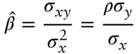
where ![]() and
and ![]() are the sample averages;
are the sample averages; ![]() and
and ![]() the standard deviations;
the standard deviations; ![]() the covariance; and
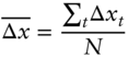
the covariance; and ![]() the correlation. The solutions (A6.4) and (A6.5) are not derived step‐by‐step here, but are easily found by noting that, with
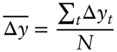
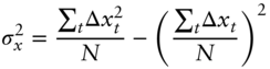
the correlation. The solutions (A6.4) and (A6.5) are not derived step‐by‐step here, but are easily found by noting that, with ![]() observations, the summary statistics needed are defined as follows,
observations, the summary statistics needed are defined as follows,

The discussion now turns to minimizing the P&L of the hedged position. That P&L, given in Equation (6.11), is repeated here for convenience,
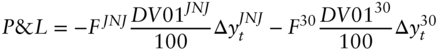
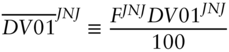
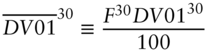
To simplify notation, write the DV01s of the bond positions as,
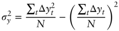
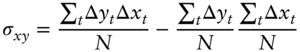
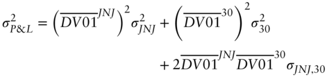
Then, with the obvious notations for variance and covariance, the variance of the P&L in (A6.12), denoted ![]() , is,1
, is,1
To minimize this variance by choosing the DV01 in the hedging bonds, differentiate (A6.15) with respect to ![]() , set the result to zero, and solve for
, set the result to zero, and solve for ![]() ,
,
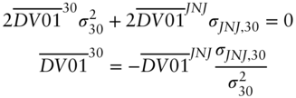
But, by inspection of Equation (A6.5), the fraction in (A6.16) is just the estimated slope coefficient in a regression of JNJ yields on 30‐year Treasury yields. Hence, the regression hedge given in Equations (6.8) or (6.10) minimizes the variance of the P&L of the hedged position.
The minimized P&L variance of the hedged portfolio can be written explicitly by substituting Equation (A6.16) into Equation (A6.15) and rearranging terms,
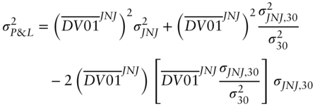
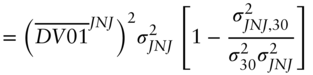
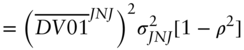
where ![]() denotes the correlation between changes in the JNJ and Treasury bond yields.
denotes the correlation between changes in the JNJ and Treasury bond yields.
The last step for this section is to show that the variance of the hedged P&L, now given in (A6.19), is equal to the squared DV01 of the bonds being hedged times the variance of the regression residuals. Starting with the definition of the regression residuals in the general regression context of (A6.1), their variance, denoted ![]() , can be expressed as follows,
, can be expressed as follows,
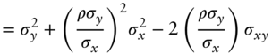
But applying Equation (A6.23) to the regression of the JNJ bonds on the 30‐year Treasury bonds, and multiplying by the DV01 of the JNJ bonds, gives exactly the right‐hand side of Equation (A6.19), which was to be proved.
A6.2 CONSTRUCTION OF PRINCIPAL COMPONENTS
The goal of this section is to illustrate how PCs are constructed with a minimum of mathematics. A slightly more rigorous mathematical treatment is given in Section A6.3. For illustration, this section uses the data from the text on daily, basis‐point changes in the five‐, 10‐, and 30‐year swap rates only. The covariance matrix, or the variance‐covariance matrix of these rate changes is,
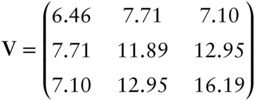
The diagonal of the matrix in (A6.24) gives the variances of the three rates, or, taking square roots, the standard deviations. The off‐diagonals give the pairwise covariances of rates, from which the correlations can be derived. For example, the volatilities of the five‐ and 10‐year rates are the square roots of 6.46 and 11.89, or 2.54 and 3.45 basis points per day, respectively, and the correlation between them is ![]() . Note, in passing, that the sum of the variances is
. Note, in passing, that the sum of the variances is ![]() , a number that appears again below.
, a number that appears again below.
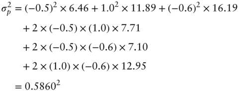
Now consider portfolio weights or loadings of ![]() 0.5, 1.0, and
0.5, 1.0, and ![]() 0.6 on the five‐, 10‐, and 30‐year rates, respectively. By the properties of variance and covariance, and with the specific covariance matrix (A6.24), the variance of this portfolio, denoted
0.6 on the five‐, 10‐, and 30‐year rates, respectively. By the properties of variance and covariance, and with the specific covariance matrix (A6.24), the variance of this portfolio, denoted ![]() , is,
, is,
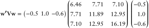
Computations like this are more conveniently written with matrix notation. Let the vector of portfolio weights be ![]() , which, in the present example, is
, which, in the present example, is ![]() , where the apostrophe denotes the transpose. Then, the same variance as computed in Equation (A6.25) can be written as,
, where the apostrophe denotes the transpose. Then, the same variance as computed in Equation (A6.25) can be written as,
Turning to the creation of the PCs, denote the first principal component by the vector of weights ![]() . Then, solve for the elements of
. Then, solve for the elements of ![]() by maximizing the variance of this PC, a'Va, such that
by maximizing the variance of this PC, a'Va, such that ![]() . Maximization ensures that, among all the PCs, the first explains the largest fraction of the sum or total variance across all rates. But there has to be some limit on the vector
. Maximization ensures that, among all the PCs, the first explains the largest fraction of the sum or total variance across all rates. But there has to be some limit on the vector ![]() , or the maximization would find portfolios with arbitrarily large variances. Enter the constraint
, or the maximization would find portfolios with arbitrarily large variances. Enter the constraint ![]() , which – along with similar constraints on other PCs – limits the risks of the PCs in a way that equates the sum of the variances of all PCs to the total variance. (See Section A6.3 for more details.) The maximization just described can be solved with the solver in Excel or some other tool to obtain that
, which – along with similar constraints on other PCs – limits the risks of the PCs in a way that equates the sum of the variances of all PCs to the total variance. (See Section A6.3 for more details.) The maximization just described can be solved with the solver in Excel or some other tool to obtain that ![]() . The variance of this PC is
. The variance of this PC is ![]() , which is 91.2% of the total variance of 34.54 given above.
, which is 91.2% of the total variance of 34.54 given above.
The second principal component, denoted by ![]() , maximizes b'Vb such that
, maximizes b'Vb such that ![]() and
and ![]() . This last constraint ensures that the portfolio represented by the second PC is uncorrelated with the portfolio represented by the first. (Again, see Section A6.3 for more details.) Solving this maximization,
. This last constraint ensures that the portfolio represented by the second PC is uncorrelated with the portfolio represented by the first. (Again, see Section A6.3 for more details.) Solving this maximization, ![]() . The variance of this PC is
. The variance of this PC is ![]() , which is 8.3% of the total variance of 34.54.
, which is 8.3% of the total variance of 34.54.
Finally, the third PC, denoted by ![]() , satisfies
, satisfies ![]() ,
, ![]() , and
, and ![]() . Solving,
. Solving, ![]() . No maximization is needed here because, by construction, this third PC explains all of the remaining total variance. The variance of this PC is
. No maximization is needed here because, by construction, this third PC explains all of the remaining total variance. The variance of this PC is ![]() , which is the remaining 0.5% of the total variance of 34.54.
, which is the remaining 0.5% of the total variance of 34.54.
The maximizations just described constrain the sum of squares of the elements of each PC to equal one. But a different scaling turns out to be convenient for interpreting the PCs: multiply each element of a PC by the volatility of that PC. In that case, the sum of squares of the elements of a PC equals its variance. In addition, after this scaling, the elements of each PC can be interpreted as the number of basis points corresponding to a one standard deviation shift in that PC. (Section A6.3 gives a more precise explanation of this point.) In the current example, the volatilities of the three PCs, from their variances computed above, are ![]() ,
, ![]() , and
, and ![]() , respectively. Multiplying the elements of the respective raw PCs by these numbers gives the scaled PCs in Table A6.1. It can then be said that a one standard deviation shock of the level PC is a 2.158‐basis‐point shift in the five‐year rate, a 3.418‐basis‐point shift in the 10‐year rate, and a 3.893‐basis‐point shift in the 30‐year rate. The scaled slope and curvature PCs can be interpreted analogously.
, respectively. Multiplying the elements of the respective raw PCs by these numbers gives the scaled PCs in Table A6.1. It can then be said that a one standard deviation shock of the level PC is a 2.158‐basis‐point shift in the five‐year rate, a 3.418‐basis‐point shift in the 10‐year rate, and a 3.893‐basis‐point shift in the 30‐year rate. The scaled slope and curvature PCs can be interpreted analogously.
TABLE A6.1 Principal Components of USD LIBOR Swap Rates, from June 1, 2020, to July 16, 2021, Using Only Five‐, 10‐, and 30‐Year Rates. Entries Are in Basis Points.
| Term | Level | Slope | Curvature |
|---|---|---|---|
| 5‐Year | 2.158 | −1.328 | 0.206 |
| 10‐Year | 3.418 | −0.303 | −0.328 |
| 30‐Year | 3.893 | 1.003 | 0.173 |
A6.3 CONSTRUCTION OF PC: MATHEMATICAL DETAILS
This section is more precise on a few claims made in the previous section at the cost of some extra mathematics. Let ![]() denote the
denote the ![]() variance‐covariance matrix of rates with elements
variance‐covariance matrix of rates with elements ![]() ; let
; let ![]() denote the
denote the ![]() matrix of principal components, with elements
matrix of principal components, with elements ![]() , or, alternatively, with three
, or, alternatively, with three ![]() column vectors
column vectors ![]() corresponding to PC
corresponding to PC ![]() ; let
; let ![]() denote the
denote the ![]() diagonal matrix with diagonal elements
diagonal matrix with diagonal elements ![]() , each equal to the variance of PC
, each equal to the variance of PC ![]() ; and let
; and let ![]() denote the
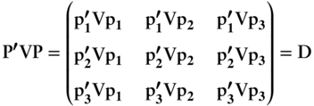
denote the ![]() identity matrix. Then, though not proved here, the construction of the PCs in the previous section guarantees that,
identity matrix. Then, though not proved here, the construction of the PCs in the previous section guarantees that,
where (A6.29) follows from (A6.27) and (A6.28).
Lemma 1: The PCs are uncorrelated.
Proof: In terms of its columns, ![]() . With this, rewrite Equation (A6.29) as,
. With this, rewrite Equation (A6.29) as,
Because ![]() is diagonal, the numbers
is diagonal, the numbers ![]() ,
, ![]() ,
, ![]() are all zero. This means that the pairwise covariances of the PCs are zero, or, equivalently, that the PCs are uncorrelated with each other.
are all zero. This means that the pairwise covariances of the PCs are zero, or, equivalently, that the PCs are uncorrelated with each other.
Lemma 2: The variance of rate ![]() equals the sum of the variance of each PC times the square of its
equals the sum of the variance of each PC times the square of its ![]() th component. Mathematically,
th component. Mathematically,
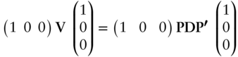
Proof: For ![]() , pre‐multiply each side of Equation (A6.27) by the
, pre‐multiply each side of Equation (A6.27) by the ![]() vector
vector ![]() and post‐multiply by the
and post‐multiply by the ![]() vector
vector ![]() . Then,
. Then,
Equation (A6.31) then follows by algebra. For ![]() , the proof is the same but with the vector
, the proof is the same but with the vector ![]() and its transpose, and for
and its transpose, and for ![]() with
with ![]() .
.
Lemma 3: The sum of the variances of the PCs equals the sum of the variances of the rates.
Proof: Adding together Equations (A6.31) for each ![]() and rearranging terms,
and rearranging terms,
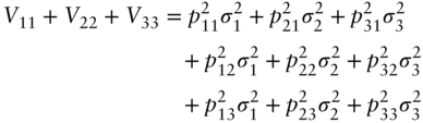
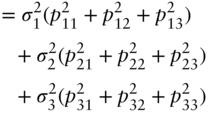
But by Equation (A6.28), the sum of squares of the elements of each PC in the brackets, ![]() , equals 1, thus proving the lemma.
, equals 1, thus proving the lemma.
Lemma 4: Defined a scaled principal component matrix, ![]() , with elements
, with elements ![]() . Then,
. Then,
Proof: This lemma follows directly from the definition of the ![]() and Equation (A6.31).
and Equation (A6.31).
To understand the significance of Lemma 4, interpret the element ![]() as the standard deviation of changes in the
as the standard deviation of changes in the ![]() th rate, in basis points, due to the scaled
th rate, in basis points, due to the scaled ![]() th PC. Then, because the PCs are uncorrelated, the standard deviation of the
th PC. Then, because the PCs are uncorrelated, the standard deviation of the ![]() th rate, with contributions from all three scaled PCs, equals the right‐hand side of Equation (A6.35). But the left‐hand side of the equation is exactly the volatility of the
th rate, with contributions from all three scaled PCs, equals the right‐hand side of Equation (A6.35). But the left‐hand side of the equation is exactly the volatility of the ![]() th rate. Hence, taken as a whole, Equation (A6.35) supports the interpretation of the elements of each scaled PCs as one standard deviation shifts in the three rates.
th rate. Hence, taken as a whole, Equation (A6.35) supports the interpretation of the elements of each scaled PCs as one standard deviation shifts in the three rates.
NOTE
- 1 Recall that for two random variables,
 and
and  , and two constants,
  and
and  , the variance of
  equals
  .
.