
CHAPTER 15
Mortgages and Mortgage‐Backed Securities
A mortgage is a loan collateralized by property. This chapter focuses on residential mortgages, through which prospective homeowners borrow money to purchase a home on the collateral of that home.
The most common mortgage loans in the United States are for 30 years and carry fixed rates of interest. They require equal monthly payments, with each allocated in part to interest (which in many cases is tax deductible) and in part to paying down principal. Mortgages also give homeowners the option to pay off or prepay all or part of the outstanding balance at any time. An implication of these contractual features is that, when mortgage rates fall, homeowners can profitably refinance their existing, high‐rate mortgages by prepaying them with money raised from new, lower‐rate mortgages. Homeowners also have to prepay when they sell a property, because the property is the collateral behind the mortgage. Details are discussed throughout the chapter, but the extent to which homeowners prepay is a key risk factor for lenders and investors: mortgages that carry an above‐market rate lose value when homeowners prepay, while those that carry a below‐market rate gain value with prepayments.
Another key risk factor is default. While mortgages are collateralized by homes, lenders can lose principal if a homeowner defaults when the value of the home is less than the outstanding balance on the mortgage. Lenders protect themselves against this scenario by lending less than the value of the home at the time of purchase, that is, by requiring that the original loan‐to‐value (LTV) ratio be less than some amount, typically 80%. The resulting buffer may not turn out to be sufficient, however, if the value of the home falls dramatically. Furthermore, with respect to any residual mortgage liability above the value of the home, lenders may or may not have recourse to the homeowner's other assets, depending on the laws of the relevant state.
The first section of the chapter describes the mortgage market in the United States, and the large role played by government agencies. Sections 15.2 to 15.4 introduce the payment conventions of mortgage loans, both fixed and floating rate, and the value of the prepayment option for fixed‐rate loans. Sections 15.5 to 15.7 discuss mortgage pools, the most basic mortgage‐backed security (MBS), along with their pricing and risk profiles. Sections 15.8 to 15.10 present the TBA and specified pools markets, and how they are used for hedging and financing. Section 15.11 deals with other types of MBS and Section 15.12 explains credit risk transfer (CRT) securities.
15.1 THE MORTGAGE MARKET IN THE UNITED STATES
Historically, banks dominated mortgage lending. They had existing relationships with potential borrowers (i.e., depositors, business owners) and their deposit base provided a relatively stable source of funds for making and holding mortgage loans. Since the Great Depression, however, US government policy has cultivated a secondary market in mortgages. The 1930s saw the creation of the Federal Housing Administration (FHA) and the Federal National Mortgage Administration, or Fannie Mae (FNMA). The FHA was created to insure lenders – for a fee – against the loss of principal or interest on approved mortgages, and FNMA was created to trade and hold FHA‐insured loans. The Veterans Administration (VA) was created in the 1940s to offer veterans federally insured mortgages, which were added to FNMA's remit. The Government National Mortgage Association – Ginnie Mae (GNMA) – and the Federal Home Loan Mortgage Corporation – Freddie Mac (FHLMC) – were created in 1968 and 1970, respectively. GNMA's mission is to package FHA‐, VA‐, and other government‐insured mortgages into MBS; to collect fees to insure those MBS; and to sell those MBS to investors. FHLMC's original purpose was to create, insure, and sell MBS from mortgages purchased from savings and loan associations.1
In their simplest form, MBS are large portfolios or pools of individual mortgages that pass through payments of interest and principal from borrowers to investors. There were several ideas behind the securitization of mortgages through MBS. First, enabling lenders to sell their mortgage loans facilitates the movement of investment funds from where they are to where they are needed. Second, a large and diversified pool of mortgages trades with much greater liquidity than would individual mortgages. Third, the guarantees described in the previous paragraph significantly increase the attractiveness of mortgages, because investors do not have to research the creditworthiness of individual homeowners nor bear that credit risk. Fourth, government can use its role in insurance and securitization to direct mortgage capital according to various policy goals, like affordable housing.
In the decades preceding the financial crisis of 2007–2009, FNMA and FHLMC were transformed into government‐sponsored enterprises (GSEs): they became privately owned, publicly traded corporations, but were heavily regulated, received many benefits from their quasi‐government status, and were required to pursue various public policy objectives. They had two business lines: the guarantee business, which made money by charging fees to package and insure MBS; and the portfolio business, which made money by borrowing in public debt markets at relatively low rates – available because of their quasi‐government status – and investing in mortgages and MBS.
GNMA, FHLMC, and FNMA are collectively called “the agencies,” and their MBS are all called “agency MBS,” even though GNMA is the only one of the three that is actually a government agency and explicitly backed by the “full faith and credit” of the federal government. In any case, from about 2000 to the financial crisis of 2007–2009, private banks, investment banks, and other mortgage lenders dramatically increased their issuance of non‐agency or private‐label MBS, particularly to pool together mortgages that were larger or less creditworthy than those acceptable for agency MBS. In fact, just before the crisis, non‐agency MBS issuance exceeded agency issuance.
During the financial crisis of 2007–2009, housing prices collapsed and many homeowners defaulted on their mortgages. Private‐label MBS, which held particularly low‐quality mortgages, suffered devastating losses, but the GSEs suffered as well. With losses on their guarantee and portfolio businesses threatening their viability, they were rescued by the US Treasury and put into conservatorship, in which state they remain to this day. Before the crisis, claims on the GSEs were not legally backed by government, but it was widely believed – and market prices reflected – that, in a crisis, the government would back those claims. And that belief was fulfilled: no holder of GSE debt or MBS lost principal or interest in the crisis.2 In this sense, the situation today is as it was before the crisis: even in conservatorship, GSE claims are not explicitly backed by the government but, should the need arise, markets expect these claims to be honored by the government.
Under conservatorship, the GSEs have continued to grow in overall size, but have been subject to a number of policy changes. First, their portfolio businesses are limited in size and scope to the facilitation of their guarantee businesses. Second, they offload some of their credit risk to the private sector through the sale of credit risk transfer securities, which are the subject of the last section of this chapter. Third, to increase liquidity, they are directed to keep their MBS similar enough to be fungible. In particular, since June 2019, MBS forward contracts, namely, TBAs, are written on uniform MBS (UMBS), which designation allows for the delivery of both FHLMC and FNMA MBS. Fourth, and most recently, provisions have been made for the GSEs to build capital in preparation for an exit from conservatorship. There are no plans in place, however, for actually effecting such an exit.
TABLE 15.1 First‐Lien Mortgages, Gross Issuance, in $Trillions.
| 2020 | Q1–Q3 2021 | |||
|---|---|---|---|---|
| Issuance | % | Issuance | % | |
| GSE MBS | 2.390 | 59.2 | 2.06 | 55.5 |
| GNMA MBS | 0.742 | 18.4 | 0.57 | 15.4 |
| Bank Portfolio | 0.869 | 21.5 | 1.02 | 27.5 |
| Private‐Label MBS | 0.038 | 0.9 | 0.06 | 1.6 |
Source: Ginnie Mae (2021), “Global Markets Analysis Report,” various months.
This brief history sets the stage for describing the US mortgage market as it stands today. Tables 15.1 and 15.2 show the extent to which agency MBS dominate the US residential mortgage market. Table 15.1 reports the gross issuance of first‐lien mortgages in 2020 and in the first three quarters of 2021.3 Starting with 2021, 70.9% of new mortgages are sold through agency MBS; 27.5% are made and held by banks; and only 1.6% are sold through private‐label MBS. The dominance of agency MBS was even greater in 2020, perhaps due to the pandemic and economic shutdowns, during which time private credit conditions were strained. Table 15.2 shows the prevalence of agency MBS with respect to amounts outstanding. About 67% of mortgages are held in agency MBS, and only 3.2% in private‐label MBS. The rightmost columns of the table separate outstanding agency MBS volumes by agency.
TABLE 15.2 Residential Mortgages Outstanding (1–4 Family), as of September 2021, in $Trillions.
| Outstanding | % | % | ||
|---|---|---|---|---|
| Agency MBS | 8.18 | 66.7 | FNMA | 40 |
| FHLMC | 34 | |||
| GNMA | 26 | |||
| Unsecuritized 1st Lien | 3.30 | 26.9 | ||
| Private‐Label MBS | 0.39 | 3.2 | ||
| Home Equity Loans (2nd Lien) | 0.40 | 3.3 | ||
| Total | 12.27 | 100.0 | 100 |
Sources: Federal Reserve Board, Financial Accounts of the United States; and Ginnie Mae (2021), “Global Markets Analysis Report,” December 2021.
Because the agencies play such a large role in the mortgage market, their underwriting criteria play an outsized role as well. Government‐insured mortgages, like those made by the FHA and VA, are called government loans. All other loans are called conventional loans. Mortgages eligible to be included in agency MBS are called conforming mortgages, while those not eligible are called nonconforming. For the GSEs, for example, at the time of this writing, conforming mortgages must have a FICO score greater or equal to 620; an LTV less than 97%; a debt‐to‐income ratio (DTI) no greater than 45%; and, for most geographical areas, a loan amount less than $647,200.4 The requisite characteristics for FHA and VA mortgages are different. In any case, jumbo mortgages, which have loan amounts greater than the “conforming balance limit,” along with mortgages of lower than conforming credit quality, have to be funded outside the agency ecosystem.5 In addition, to the extent that the GSEs limit purchases of mortgages with certain characteristics, like those funding second homes or investment properties, private markets have the opportunity to satisfy the residual demand.
Table 15.3 shows averages of selected characteristics of loans to first‐time homebuyers for the purposes of purchasing a home (rather than refinancing an existing mortgage). Loan characteristics do not vary much across FNMA and FHLMC, because, as mentioned before, their business models are converging. GNMA loans are smaller and, by standard metrics, less creditworthy, with significant variation across FHA, VA, and other government‐guaranteed loans.
Deposit franchises give banks competitive advantages in making and holding mortgage loans. These advantages are much less pronounced, however, for originating conforming mortgages, that is, for arranging mortgages with borrowers and then selling those mortgages into agency MBS. With the increasing dominance of agency MBS, therefore, the market share of nonbank originators has steadily increased, from less than 25% in 2007 to more than 75% toward the end of 2021.6 In fact, a rough calculation assuming a 25% bank share of agency MBS originations, and mortgage gross issuance as described in Table 15.1, that is, 71% for agency MBS and 27.5% for bank loan portfolios, gives an overall bank participation in mortgage issuance of 25% times 71% plus 27.5%, or about 45%.
TABLE 15.3 Average Characteristics of First‐Time Homebuyer Purchase Loans, as of December 2020.
| Within GNMA MBS | ||||||
|---|---|---|---|---|---|---|
| FNMA | FHLMC | GNMA | FHA | VA | Other | |
| Loan Amount ($) | 305,134 | 264,303 | 245,013 | 237,630 | 299,448 | 174,011 |
| FICO Score | 750.4 | 744.7 | 688.5 | 678.6 | 713.3 | 701.1 |
| LTV (%) | 87.7 | 88.0 | 96.8 | 95.5 | 99.6 | 99.4 |
| DTI (%) | 34.1 | 34.4 | 41.5 | 43.1 | 39.5 | 34.9 |
Source: Ginnie Mae (2021), “Global Markets Analysis Report,” February.
Nonbank origination channels are classified into three groups: retail, broker, and correspondent. Retail originators contact borrowers directly. Broker originators provide various services to independent brokers who seek out and find potential borrowers. And correspondent originators buy loans from smaller banks and credit unions.
This market overview concludes with mortgage servicers. Servicers receive ongoing fees to administer mortgage loans; keep in touch with borrowers; pass payments from borrowers to investors; help borrowers through loan modifications or forbearance; and, in the case of missed payments, temporarily advance funds to investors. Lenders can either keep the servicing rights to a loan or sell the rights to another entity. Arguments for keeping the rights include their performing as a hedge to an origination business. First, servicing provides steady income through periods of slow origination. Second, when refinancings decrease servicing income (by extinguishing existing mortgages), income from refinancing originations increases. Another reason originators keep servicing rights is to keep in touch with borrowers who may be contemplating refinancing. In that way, lenders can recapture refinancing, that is, market their own refinancing products with the goal of preventing borrowers from refinancing with a different originator.
15.2 FIXED‐RATE MORTGAGE LOANS
Though terms of 10, 15, and 20 years are also available, the most common mortgage is a 30‐year, fixed‐rate, level payment mortgage. For example, a homeowner might borrow $100,000 from a bank at 4.5% and agree to make payments of $506.6853 every month for 30 years. (The extra decimal places are given to help the reader reproduce the calculations to follow.) The loan rate and the monthly payment are related by,
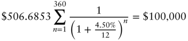
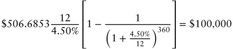
where Equation (15.2) follows by applying Equation (A2.16).
These equations say that, at a rate of 4.5%, the present value of the monthly payments on the mortgage over its 30‐year or 360‐month life equals the initial loan amount of $100,000. This relationship is simply a market convention to define a monthly payment from a mortgage rate, just as price is quoted given yield to maturity or vice versa. Truly pricing a mortgage loan is much more complicated, of course, with the need to account for a term structure of risk‐free rates, the value of the prepayment option, and a spread or term structure of spreads to reflect credit risk.
The market convention of a single rate to describe a mortgage loan is also used to divide its monthly payments into interest and principal components. Table 15.4 gives selected rows of the amortization table for the mortgage just described, with the monthly payment rounded to $506.69. The starting balance is $100,000. The interest component of the first payment is the interest on that starting balance at a rate of 4.50%, that is, ![]() . The principal component of the first payment is simply the total monthly payment, fixed at $506.69, minus the interest component of $375.00, or $131.69. Given this breakdown, the ending balance of the loan at the end of the first month is the starting balance minus the first principal payment, that is, $100,000 minus $131.69, or $99,868.31. For the second payment, interest on the outstanding balance at the end of the first month is
. The principal component of the first payment is simply the total monthly payment, fixed at $506.69, minus the interest component of $375.00, or $131.69. Given this breakdown, the ending balance of the loan at the end of the first month is the starting balance minus the first principal payment, that is, $100,000 minus $131.69, or $99,868.31. For the second payment, interest on the outstanding balance at the end of the first month is ![]() ; the principal payment is
; the principal payment is ![]() ; and the ending balance is
; and the ending balance is ![]() . Subsequent payments are handled analogously.
. Subsequent payments are handled analogously.
Appendix A15.1 shows that, using this method of amortizing principal, the ending balance at any time equals the present value of all remaining payments discounted at the original interest rate. Applied to the example, the balances at the end of five years, or 60 months (300 months remaining), and at the end of 10 years, or 120 months (240 months remaining), are shown in the table and can be computed, respectively, by the following equations,
TABLE 15.4 Selected Rows of a Mortgage Amortization Table for a 30‐Year $100,000 Mortgage at 4.5%. The Total Monthly Payment Is $506.69. Entries Are in Dollars.
| Payment | Interest | Principal | Ending |
|---|---|---|---|
| Month | Payment | Payment | Balance |
| 100,000.00 | |||
| 1 | 375.00 | 131.69 | 99,868.31 |
| 2 | 374.51 | 132.18 | 99,736.14 |
| 3 | 374.01 | 132.67 | 99,603.46 |
| 4 | 373.51 | 133.17 | 99,470.29 |
| 5 | 373.01 | 133.67 | 99,336.62 |
| 60 | 342.46 | 164.23 | 91,157.92 |
| 120 | 301.11 | 205.58 | 80,089.43 |
| 358 | 5.66 | 501.03 | 1,007.70 |
| 359 | 3.78 | 502.91 | 504.79 |
| 360 | 1.89 | 504.79 | 0.00 |
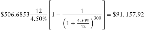
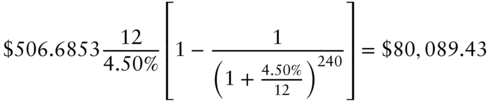
Figure 15.1 depicts the amortization of this mortgage graphically. For each month, against the left axis, the height of the dark‐shaded area represents the principal component of that month's payment; the height of the light‐shaded area represents the interest component; and the total height, or sum, equals the fixed total payment of $506.69. The black curve, against the right axis, gives the ending balance or principal outstanding at the end of each month. The figure clearly illustrates the banker's adage that “interest lives off principal,” that is, as principal is paid off, interest payments decline. Interest constitutes $375.00/$506.69 or 74.0% of the first monthly payment; $342.46/$506.69 or 67.6% of the 60th payment; $301.11/$506.69 or 59.4% of the 120th payment; etc.; and $1.89/$506.69 or 0.4% of the final payment. While not shown in the figure, the higher the loan rate, the greater the monthly payment, and the greater the proportion of each payment that is dedicated to interest.
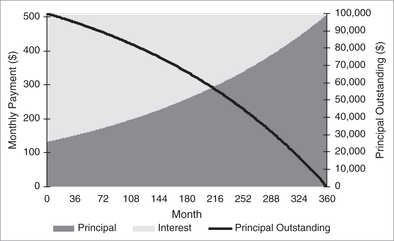
FIGURE 15.1 Amortization of a 30‐Year $100,000 Mortgage at 4.5%.
15.3 ADJUSTABLE‐RATE MORTGAGES
While the overwhelming majority of mortgages are fixed‐rate mortgages, adjustable‐rate mortgages (ARMs) are available as well. The distinguishing feature of an ARM is that the mortgage interest rate can vary over time, but the details of the loan contract can be relatively complex. To illustrate, consider one relatively common variety of ARMs, a 30‐year 5/1 hybrid ARM with a 2/2/5 cap structure.
The phrase “hybrid ARM” means that the mortgage rate is fixed for some number of years before it begins to vary according to some set of rules. In a 5/1 hybrid ARM, for example, i) the mortgage rate is fixed for the first five years; and ii) at the end of that time, and every one year thereafter, the mortgage rate is reset. The new mortgage rate at each reset equals some rate benchmark, like the one‐year rate on US Treasury bonds, plus a gross margin, which is set and fixed at the initiation of the mortgage. To put some numbers on this, say that the gross margin is 2.75%, the index is the one‐year Treasury rate, and the one‐year Treasury rate applied to the reset is 0.25%. In that case, the mortgage rate over the subsequent year is set to 3.00%. The Treasury rate is typically observed with a lookback, perhaps 45 days, so that the borrower knows the applicable mortgage rate sometime before it goes into effect.
Once the mortgage rate of an ARM is set, the monthly payments are calculated as in the case of a fixed‐rate mortgage. To be more specific, consider the 30‐year 5/1 hybrid ARM example at the end of year five. Say that the outstanding balance is $80,000 (computed based on the mortgage rate over the first five years) and that the mortgage rate is to be reset to 3%. The remaining maturity, of course, is 25 years. The mortgage payment is then computed such that the present value of that monthly payment over the next 25 years or 300 months equals $80,000. It is as if a new fixed‐rate mortgage for the outstanding balance and the remaining term is being offered at the new mortgage rate.
The 2/2/5 cap structure of the example limits the extent to which the mortgage rate can change over the life of the ARM. The three numbers refer to the initial adjustment rate cap, the periodic adjustment rate cap, and the lifetime adjustment rate cap, respectively. The initial adjustment rate cap of 2% says that the mortgage rate for the sixth year of the mortgage, set at the end of year five, cannot increase or decrease the rate by more than 2% (i.e., a rate of 3% can neither rise above 5% nor fall below 1%). The periodic adjustment rate cap of 2% says that, at the end of any year, the rate cannot increase or decrease by more than 2%. And the lifetime adjustment cap of 5% says that, over the life of the mortgage, the rate cannot increase by more than 5%. Furthermore, the mortgage rate is typically constrained to remain above the gross margin rate.
ARMs typically offer lower initial interest rates than fixed‐rate mortgages but expose homeowners to the risk that rates increase. The average loan size of ARMs is significantly higher than that of fixed‐rate mortgages, perhaps because wealthier, larger borrowers have more tolerance for interest rate risk. In recent years, the volume of ARMs, as a percentage of all mortgages, has fallen to the single digits. Perhaps, with mortgage rates near historic lows, borrowers perceive the risk of higher rates as exceeding the potential benefit of lower rates. Also, ARMs are still held in some disrepute from the financial crisis of 2007–2009. In the years leading up to the crisis, many people were tempted to buy into the housing boom by the relatively low initial payments of ARMs, accentuated by teaser rates, a practice at the time of offering particularly low rates over the first year or two of the ARM. Many homebuyers overextended themselves through these products and faced default as the rates on their ARMs reset higher and the housing market collapsed.
15.4 PREPAYMENTS
The prepayment option allows a homeowner to pay off or prepay a mortgage, in whole or in part, at any time, by paying the bank the outstanding balance. In the example of Table 15.4, the homeowner may pay the bank $80,089.43 at the end of 10 years and has no further obligations under the mortgage. But if the mortgage rate has fallen over those 10 years, say to 3.50%, then – using 3.50% instead of 4.50% in Equation (15.4) – the present value of the remaining payments will have risen to $87,365.60. Hence, in that scenario, the prepayment option is in‐the‐money: the homeowner may pay the bank $80,089.43 to extinguish a liability with a present value of $87,365.60. On the other hand, if the mortgage rate has stayed the same or risen above 4.50% after those 10 years, then the present value of the mortgage liability will be less than $80,089.43, and the homeowner will have no incentive to prepay.
In practice, of course, most homeowners with mortgages do not have the cash to pay off an existing mortgage. They can take advantage of an in‐the‐money prepayment option, however, by refinancing an existing mortgage. Continuing with the example, the homeowner might borrow $80,089.43 at the then‐prevailing mortgage rate of 3.50%, and then use that cash to prepay the existing 4.50% mortgage. In that case, one way to describe the savings to the homeowner is in terms of the reduction in monthly mortgage payments: using the math given earlier, the monthly payment on a 20‐year $80,089.43 mortgage at 3.50% is $464.48, which is $42.21 a month less than the $506.69 on the existing mortgage. Note that the homeowner is not constrained to refinance with the bank that extended the original mortgage. Another originator might have brought the refinancing opportunity to the attention of the homeowner and might be offering a lower rate or lower transaction costs.
Refinancing activity is usually constrained by the value of the home. Assume, in the example, that the homeowner can economically borrow only 80% of the value of the home; that is, the LTV has to be less than or equal to 80%. In that case, the value of the home when the existing $100,000 mortgage was extended had to have been greater or equal to $125,000, and 10 years later, at the time of the $80,089.43 refinancing, has to be above $100,112. In fact, if the value of the home after 10 years is greater than that $100,112, the homeowner might do a cash‐out refinancing, which means borrowing more money than the outstanding balance of the existing mortgage. In the example, if the home is still worth $125,000 at the time of the refinancing, the homeowner could borrow $100,000 in the refinancing mortgage, pay off the existing mortgage with $80,089.43, and take the residual $19,910.57 in cash to be used for other purposes. Increasing leverage in this way can, of course, be dangerous. Rising property values in the run up to the financial crisis of 2007–2009 encouraged significant volumes of cash‐out refinancings that left many homeowners with negative home equity when home values subsequently plummeted. In fact, in response to that experience, the GSEs currently do not accept cash‐out refinancing loans with LTVs greater than 80%.
When interest rates are low, refinancings can generate significant mortgage volumes. Over the most recent period of falling rates, refinancings as a percentage of residential mortgage originations increased from 33% in 2018, to 46% in 2019, and to 65% in the first half of 2020.7
Homeowners sometimes exercise prepayment options with curtailments, but these are not nearly so significant as refinancings. These prepayments take place mostly when homeowners pay off very old, low‐balance mortgages, simply to own a home free and clear of debt. Financial considerations, like the existing mortgage rates relative to market mortgage rates become secondary, lost in the excitement of literal or figurative mortgage‐burning parties.
Prepayments occur for other reasons as well, most notably turnover and defaults. Turnover refers to the ongoing economic activity of selling and buying homes. Turnover generates prepayments, because homes, which are the collateral for mortgages, cannot be sold until the mortgages are paid off. Disasters that destroy homes also generate turnover prepayments, because mortgages become due in those situations as well.
Defaults refer to cases in which homeowners fail to make contractual mortgage payments. In these cases, for mortgages packaged into MBS, interest and principal are advanced by the servicer and ultimately paid by the insurer. Hence, from the perspective of mortgage investors, defaults are economically equivalent to early payments of principal, rather than as losses to principal invested.
15.5 MORTGAGE POOLS
The simplest form of an MBS is a mortgage pool, which is a portfolio of individual mortgages through which payments of interest and principal are passed from borrowers to investors. Borrowers make payments by the first of each month, which servicers pay to investors on the 25th of each month, or on the first business day thereafter.8
Table 15.5 presents descriptive statistics as of December 2021 for three 30‐year FNMA pools, that is, portfolios of mortgages with approximately 30 years to maturity securitized by FNMA. Consider first the two pools, CA2797 and MA3538, which were both issued in November 2018 and mature 30 years and one month later, in December 2048. Metrics in the table can be shown as “current,” that is, as of the report date, in this case December 2021, or as “original,” that is, as of the issue date, in this case, November 1, 2018. The table shows the WAM or weighted‐average maturity of the loans in the pool and the WALA or weighted‐average loan age, where each loan is weighted by its balance or principal outstanding as a percentage of total pool balance. In the simplest possible case, every loan in a pool would mature in exactly 30 years or 360 months as of the date of issue – giving an original pool WAM of 360 and WALA of zero – and, as of the report date, 37 months later, a current WAM of ![]() and WALA of 37. Reality is more complex, however, because 30‐year pools may be issued containing mortgages ranging in maturity from 181 to 361 months, and many mortgages prepay and drop out of pools between the issue and report dates.9
and WALA of 37. Reality is more complex, however, because 30‐year pools may be issued containing mortgages ranging in maturity from 181 to 361 months, and many mortgages prepay and drop out of pools between the issue and report dates.9
The next row of Table 15.5 gives the coupons of the CA2797 and MA3538 pools as 4.5% and 5.0% respectively. The coupon of a pool is the mortgage rate paid to investors. As a pass‐through security, pool interest from the borrowers is paid to the investors, but only after subtracting a guarantee fee or g‐fee for the insurer, in this case FNMA, and a servicing fee for the servicer. The next row in the table, gives the WAC, or weighted‐average mortgage rate of the loans in the pool. As of the issue date, the WAC of CA2797 was 4.924%, leaving 42.4 basis points worth of fees above the 4.500% coupon paid to investors. The acronym WAC stands, for “weighted‐average coupon” and is unfortunate: the word “coupon” most often refers to the rate on a pool paid to investors, while WAC, as just mentioned, is a weighted average of the rates on the underlying loans. In any case, the current WAC of CA2797, at 4.198%, is marginally lower than the original WAC, which means that, on average, loans with marginally higher rates prepaid faster between the issue and report dates. For MA3538, however, the original WAC is slightly less than the current WAC, which means that loans with marginally lower rates prepaid faster.
The next section of Table 15.5 describes the principal amount of the pools, their underlying loans, and experienced prepayments. At issue, CA2797 had 943 loans at an average size or loan principal amount of $138,913, for a total pool balance of about $131 million. As of the report date, the number of loans had fallen to 339, and the pool balance to about $44 million. These numbers reveal a significant rate of prepayment. Using the formulae presented earlier, a $100,000 30‐year mortgage at a rate of 5% amortizes down to an outstanding balance after 37 months of $95,204. This scheduled amortization can be summarized with a factor, or remaining fraction of original principal, of ![]() or 0.952. The factor of CA2797 after 37 months, however, is
or 0.952. The factor of CA2797 after 37 months, however, is ![]() or 0.333. That CA2797 prepaid heavily is not particularly surprising, as mortgage rates fell significantly between November 2018 and December 2021. That the average loan size fell from $138,913 to $128,773 indicates that larger loans prepaid more rapidly than smaller loans. This aspect of prepayments is accepted as broadly applicable: homeowners with larger loan amounts are, on average, wealthier and more financially sophisticated and, therefore, more able to take advantage of refinancing opportunities.
or 0.333. That CA2797 prepaid heavily is not particularly surprising, as mortgage rates fell significantly between November 2018 and December 2021. That the average loan size fell from $138,913 to $128,773 indicates that larger loans prepaid more rapidly than smaller loans. This aspect of prepayments is accepted as broadly applicable: homeowners with larger loan amounts are, on average, wealthier and more financially sophisticated and, therefore, more able to take advantage of refinancing opportunities.
TABLE 15.5 Descriptive Statistics for Three 30‐Year FNMA Pools, as of December 2021.
| CA2797 | MA3538 | AI4813 | ||||
|---|---|---|---|---|---|---|
| Pool | Current | Original | Current | Original | Current | Original |
| Payment Terms | ||||||
| Issued | 11/1/2018 | 11/1/2018 | 6/1/2011 | |||
| Maturity | 12/1/2048 | 12/1/2048 | 6/1/2041 | |||
| WAM (months) | 314 | 360 | 319 | 359 | 214 | 359 |
| WALA (months) | 37 | 37 | 126 | |||
| Coupon (%) | 4.500 | 5.000 | 4.500 | |||
| WAC (%) | 4.918 | 4.924 | 5.772 | 5.768 | 4.935 | 4.942 |
| Loans and Prepayments | ||||||
| Amount ($mm) | 43.654 | 130.995 | 105.011 | 594.633 | 29.374 | 266.801 |
| Number | 339 | 943 | 422 | 2,050 | 311 | 2,037 |
| Avg. Size ($) | 128,773 | 138,913 | 248,841 | 290,065 | 94,451 | 130,977 |
| 1mo CPR (%) | 24.6 | 46.9 | 21.9 | |||
| Credit Quality | ||||||
| WAOCS | 740 | 678 | 758 | |||
| SATO (bps) | −6 | 78 | −6 | |||
| WAOLTV (%) | 79 | 80 | 70 | |||
| Additional Statistics | ||||||
| Own/2nd/Inv (%) | 91/6/3 | 86/3/11 | 86/9/5 | |||
| Buy/Refi (%) | 75/25 | 42/58 | 53/47 | |||
| R/C/B (%) | 63/25/13 | 42/46/12 | 38/58/4 | |||
| State (%UPB) | TX: 9.0 | CA: 20.6 | CA 10.6 | |||
| FL: 8.7 | TX: 13.5 | TX 10.0 | ||||
| PA: 6.5 | FL: 13.4 | FL 6.4 | ||||
| Pricing | ||||||
| Price | 109.783 | 108.963 | 110.309 | |||
| OAS | 90.1 | 113.0 | 86.5 | |||
| OAD | 3.98 | 3.18 | 4.26 | |||
WAM: weighted‐average maturity; WALA: weighted‐average loan age; WAC: weighted average coupon; CPR: conditional prepayment rate; WAOCS: weighted‐average original credit score; SATO: spread at origination; WAOLTV: weighted‐average original loan‐to‐value ratio; Own/2nd/Inv: owner‐occupied, second home, investment property; R/C/B: retail, correspondent, broker; UPB: unpaid balance.
The MA3538 pool could reasonably be expected to prepay faster than CA2797. First, the loans underlying MA3538 have higher loans rates, which – subject to a caveat discussed next – increase the incentive to refinance. Second, the average loan size of MA3538 is much higher and, as just mentioned, larger loans tend to prepay faster. And, indeed, MA3538 has prepaid much faster. Its factor of ![]() or 0.177 is a lot lower than the 0.333 factor of CA2797.
or 0.177 is a lot lower than the 0.333 factor of CA2797.
The next row of the table gives the CPR, the conditional prepayment rate or the constant prepayment rate, over the most recent month. CPR is an annualized measure of the speed of prepayments, which is intricately related to another measure, the SMM or single monthly mortality rate. Define ![]() as the percentage of principal outstanding that is prepaid during month
as the percentage of principal outstanding that is prepaid during month ![]() . Note that prepaid principal does not include scheduled or amortized principal payments, like those described in Table 15.4. CPR then annualizes SMM by assuming that SMM is constant over the year. Under that assumption, the principal not prepaid over one month is
. Note that prepaid principal does not include scheduled or amortized principal payments, like those described in Table 15.4. CPR then annualizes SMM by assuming that SMM is constant over the year. Under that assumption, the principal not prepaid over one month is ![]() ; principal not repaid over 12 months is
; principal not repaid over 12 months is ![]() , and prepayments over 12 months are given by,
, and prepayments over 12 months are given by,
While CPR is an annualized rate, it is reported monthly based on the prepayments during that month. For example, if a pool prepaid 2% of its outstanding principal above its amortizing principal in a given month, it is prepaying at an annualized speed or CPR given by Equation (15.5), that is, 21.53%. CPR is less than 12 times the monthly rate of 2%, or 24%, because of the compounding in Equation (15.5): the amount remaining each month is not 98% of the original principal balance, but only of the principal balance after some number of months of prepayments. A CPR can be computed over several months as well. Say, for example, that the SMMs for a particular pool over three months were 2%, 2.5%, and 3%. Then the CPR of that pool over that three‐month period is,
where raising the product of the three monthly survival rates to the fourth power gives the annual survival rate. Finally, then, returning to Table 15.5, the most recent monthly CPR of MA3538, at 46.9%, is much greater than the 24.6% CPR of CA2797.
The next three rows of the table relate to pool credit quality. The first, WAOCS (weighted‐average original credit score), gives the weighted‐average credit or FICO scores of the borrowers with loans in the pool. The second, SATO or spread at origination, gives the weighted‐average spread of the loan rates over a mortgage index rate at the time of origination. By these two metrics, the loans in MA3538 are significantly less creditworthy than those in CA2797. In fact, the 84.4‐basis‐point difference between the original WACs of the pools is approximately equal to the 84‐basis‐point difference in their SATOs. This, then, is the caveat in attributing faster prepayments of MA3538 to its higher coupon rate. Because that higher coupon is most likely due to inferior credit, refinancing the loans in MA3538 will likely require a higher rate as well, meaning that the incentive to refinance – which is closely related to the difference between the existing mortgage rate and the available refinancing rate – may not be much greater for MA3538 than for CA2797. Furthermore, lower credit loans are thought to prepay relatively slowly, because homeowners with lower credits might find it more difficult to obtain refinancing loans. In any case, with respect to the other metric of loan quality, WAOLTV (weighted‐average original LTV), the two pools are quite similar, at 79% and 80%.
The next several rows of Table 15.5 report a selection of additional pool statistics. These and other statistics, not shown here, are studied in great detail by market participants in an attempt to determine the speed at which a pool will prepay. The first row of this section of the table gives the percentages of loans for owner‐occupied homes, for second homes, and for investment properties. The second gives the percentage of loans used to purchase the home and the percentage used to refinance. The third gives the percentages in each of origination channels described earlier, and the fourth gives the largest percentages of unpaid balance by state. Exactly how these statistics predict prepayments is part of the art of prepayment modeling, but some broad outlines are described here. Rates on loans for investment properties are typically higher than for owner‐occupied properties, reflecting the greater propensity of investors to walk away from distressed situations. Across mortgages with the same coupon, therefore, investor properties, which have to be refinanced at relatively high rates, face a lower refinancing incentive and, consequently, refinance at lower speeds. With respect to turnover, however, investor properties prepay relatively fast: investors are on the lookout for opportunities to sell properties at a profit, and they do not bear the costs of changing residences to do so. Loans for the purpose of refinancing might prepay faster, because homeowners who have refinanced already might have greater propensity to do so. Brokered originations might refinance faster, because, with no stake in the servicing fees, that is, with no losses from extinguishing existing mortgages, brokers might have the greatest incentive to generate new refinancing originations. This effect is countered, however, by the efforts of originators, mentioned earlier, to recapture refinancings. Finally, loans in some states seem to prepay faster than others, controlling for the other effects discussed so far. These differences across states are usually attributed to differences in the costs of closing mortgages, which are composed of various taxes and fees. For example, average closing costs in New York are among the highest, and prepayments there are particularly slow, while average closing costs in California are relatively low and prepayment speeds there are particularly fast.
15.6 PREPAYMENT MODELING
The complex behavior of prepayments, combined with their importance in mortgage valuation, has given rise to a large industry of building models to predict prepayments as a function of interest rates and other variables. While some highlights are presented in this section, and Appendix A15.2 presents some of the more technical issues encountered, a fuller description is beyond the scope of this chapter.
Prepayment models are often divided into separate modules, one for each driver of prepayments. The most notable drivers, mentioned earlier, are refinancing, turnover, defaults, and curtailments. Traditionally, a module makes a set of assumptions that depend on various parameters. These parameters are then estimated historically, using the vast amount of data available on the prepayment behavior of mortgage pools. Some parameters might also be implied from prevailing market prices of various pools. Most recently, artificial intelligence and machine learning technologies have also been brought to bear on the problem of predicting prepayments.
At the heart of most refinancing modules is an S‐curve, which describes refinancings, often in terms of CPR, as a function of some incentive function. The incentive function might be the difference between the existing mortgage rate and the current mortgage rate; the ratio of the existing rate to the current rate; the present value of the savings from refinancing; or even the monthly savings from such a refinancing. The S‐curve than maps the refinancing incentive into a CPR. Figure 15.2 shows the S‐curves of a particular model for the three pools summarized in Table 15.5. The horizontal axis here is simply the change in the current mortgage rate. Because existing mortgage rates are fixed, of course, rising current mortgage rates imply less of an incentive to prepay, while falling current mortgage rates imply more of an incentive to prepay.
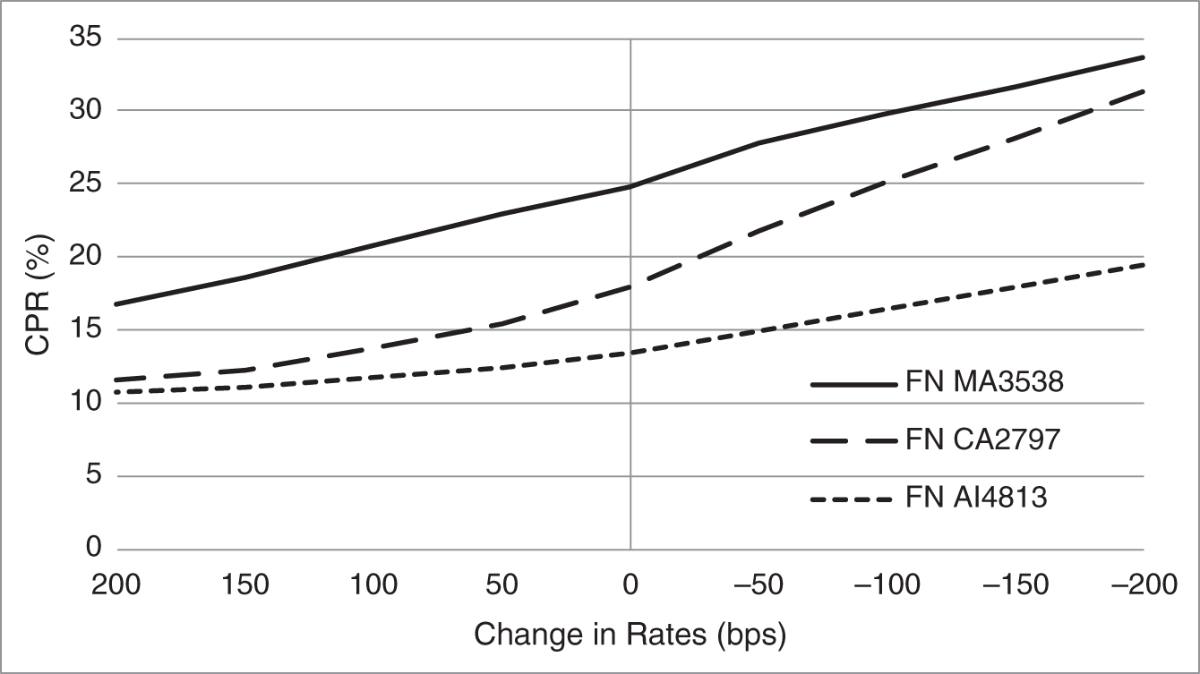
FIGURE 15.2 Refinancing S‐Curves for Three Mortgage Pools.
The name “S‐curve” comes from the shape of the functions. For large increases in rates, or, equivalently, very low incentives and high current mortgage rates, CPR is very low, while for large decreases in rates, or very high incentives and low current mortgage rates, CPR is very high. The curves in the figure do not look much like an “S,” but the faster a curve moves from low to high CPR, the more the curve looks like something like an “S.” In any case, the shape of the S‐curve is different for each pool, and can depend on all of the characteristics discussed in the context of Table 15.5 (e.g., average loan size, creditworthiness). According to the models behind Figure 15.2, MA3538 prepays faster than CA2979, but, for a large enough decrease in mortgage rates, the CPR of CA2797 comes close to catching up. Figure 15.3 shows some empirical evidence with which these two S‐curves might have been estimated. As the current coupon mortgage rate (which is defined herein) declined dramatically from between 3.50% and 4.00% at the time of origination to less than 1.50% in fall 2020, the CPR of both pools rose dramatically. But MA3538 prepaid faster. As rates stayed low and increased somewhat, prepayments on both remained relatively high, but MA3538, on average, continued to prepay faster. By the way, this figure also shows why refinancing models are not cast as an optimization problem. If homeowners exercised their prepayment options with the efficiency of bond issuers exercising their call options, the pools in the figure would have experienced such dramatic prepayments through September 2020 that little to no principal would remain outstanding.
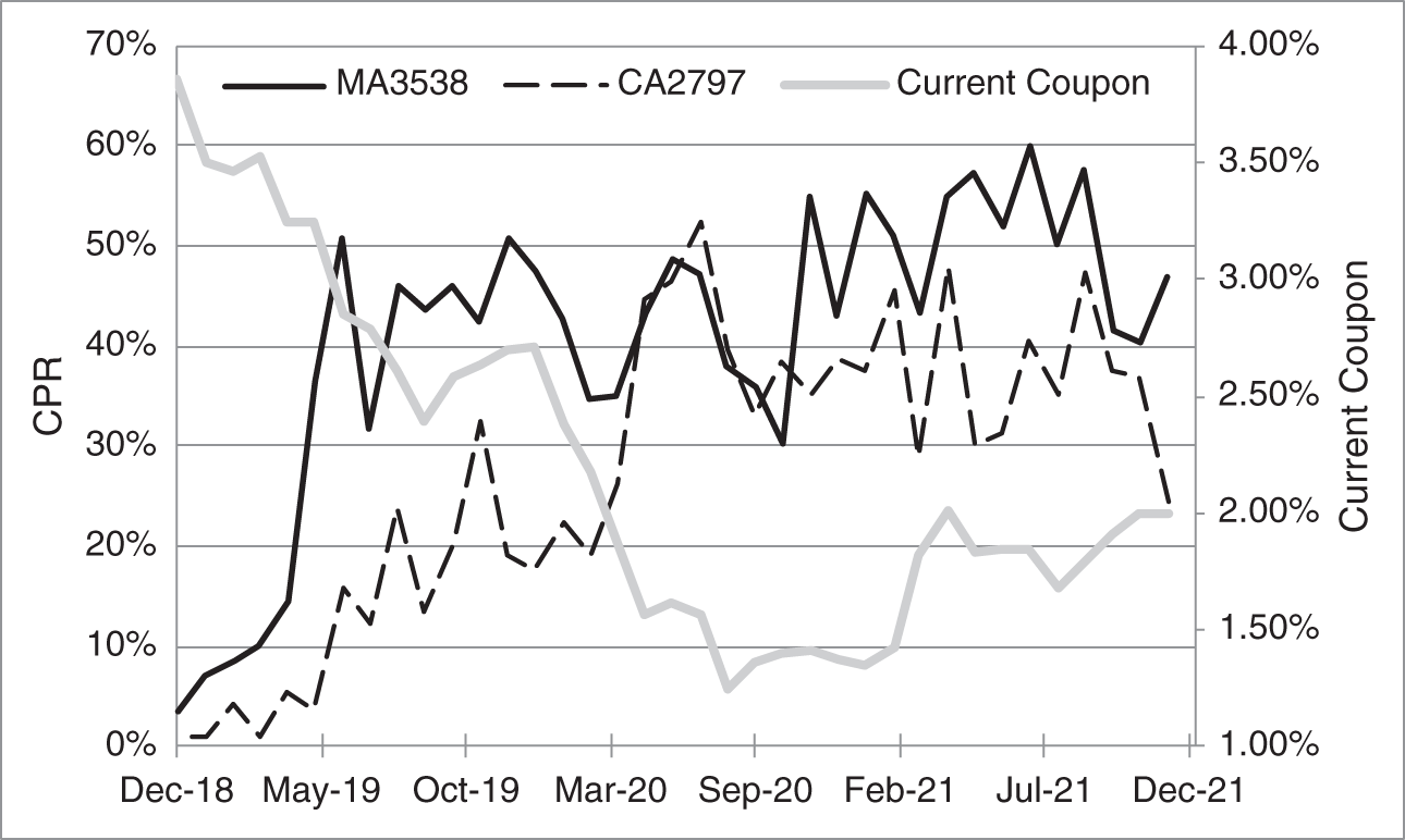
FIGURE 15.3 One‐Month CPR for FN MA3538 and FN CA2797 and the 30‐Year Current Coupon Rate.
Returning to Figure 15.2, the CPR of AI4813 is much lower than that of the other pools and picks up relatively slowly as rates decline. Contrasting its characteristics with those of CA2797 and MA3538, Table 15.5 reports that AI4813 was issued in June 2011, with a correspondingly shorter current WAM and WALA than the other pools. Its current WAC is essentially the same as that of CA2797. The current average loan size of AI4813 is significantly smaller than that of either of the other pools, while its creditworthiness is marginally higher than that of CA2797. AI4813 is between the other two pools with respect to loan purpose, and the percentage of brokered originations is somewhat lower. The most likely explanation for the lower S‐curve of AI4813, therefore, is not these loan characteristics but rather a prepayment phenomenon known as burnout.
When a seasoned or older pool has been through a period of relatively low rates and experienced significant prepayments, it is most likely that the homeowners with the greatest propensity to prepay have already prepaid and are no longer in the pool. With the remaining loans in the pool less likely to prepay, the pool experiences some degree of burnout. Figure 15.4 illustrates burnout in the case of AI4813. As the mortgage rate fell from about 4.00% at the time of origination to between less than 2.00% and about 2.50% from late 2012 through the first hal of 2013, CPR increased dramatically, to a peak of about 34%. Rates then rose and fell again to between 2.00% and 2.50%, and CPR reached a similar peak of over 30% in fall 2016. Rates subsequently rose a second time, peaking in November 2018, before starting on a third and more dramatic decline. This time, however, even when rates fell to 2.00%, CPR never rose above 20%. As a burned‐out pool, it was not until sometime after mortgage rates has fallen to new lows of below 1.50% that prepayments rose again, this time to a peak above 40%. From a modeling standpoint, burnout introduces the significant complication that the S‐curve depends not only on the current characteristics of a pool but also on the history of rates experienced by the pool.
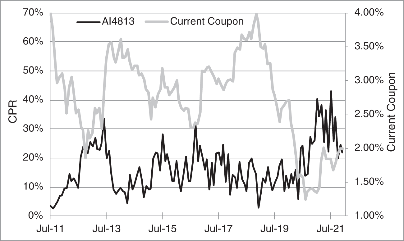
FIGURE 15.4 One‐Month CPR for FN AI4813 and the 30‐Year Current Coupon Rate.
Mortgage professionals might also take the surge of AI4813 prepayments in 2021, as depicted in Figure 15.4, as evidence of a media effect. After a precipitous decline in mortgages rates, or after a decline in which mortgage rates reach new lows, media reports and party conversations encourage even those borrowers with low propensities to refinance to do so. Once again, this effect considerably complicates the determination of the S‐curve.
Another module of prepayment modeling captures turnover. A common approach to these modules is to start, at issue, from some base rate of turnover, which increases over time according to a seasoning ramp. This choice reflects the empirical regularity that homeowners are unlikely to move soon after taking out a mortgage. The exact specification of the seasoning ramp can depend on factors other than mortgage age, most obviously the season, as homeowners are more likely to move at certain times of the year, like soon before schools open rather than soon after. While prepayments due to turnover are for the most part independent of mortgage rates, there is a significant interaction. Borrowers are less likely to move if they have below‐market mortgage rates, that is, if they would pay significantly higher mortgage rates after selling their homes and buying new ones. This phenomenon is known as the lock‐in effect.

FIGURE 15.5 Prices of FN CA2797 Versus the Five‐Year Treasury Rate, from November 30, 2018, to February 28, 2020, and from May 18, 2020, to December 21, 2021.
As for modules for default, only a few observations are recorded here. Investors in agency MBS experience defaults as prepayments, but defaults are nevertheless tracked and modeled separately, as involuntary rather than voluntary prepayments. Inputs to these models include credit scores at the time of origination, because credit scores are typically not updated after issuance. While LTVs are not updated either, they can be estimated over time, at the loan level, by using data on home prices in a relevant region. Home prices are important in determining defaults, because a homeowner without cash – but with a home valued in excess of its mortgage balance – can sell the home and pay off the mortgage rather than default.
15.7 MORTGAGE PRICING, SPREADS, AND DURATION
Combining a prepayment model with a risk‐neutral model of the term structure, MBS can be computed as the expected discounted value of their cash flows. Because the model price of a given MBS typically does not perfectly match its market price, an option‐adjusted spread (OAS) is defined as the spread that, when added to the initial, benchmark term structure, results in a model MBS price that equals the market price. OAS is the equivalent of bond spread introduced in Chapter 3 and discussed in Chapter 7. In particular, the OAS can be interpreted as the extra return earned when interest rate risk is correctly hedged by the model with securities that are fairly priced by the model.
A straightforward use of OAS is to buy cheap securities, those with high OAS; to sell rich securities, those with low OAS; and, more aggressively, to engage in relative value trades that simultaneously buy high‐OAS and short low‐OAS securities. A practical challenge to investing and trading with OAS is model error or misspecification. It is unusual for a model to find that a particular MBS is cheap or rich, while other MBS, with similar characteristics, are fair. More usual is to find that a particular sector, for example, pools with high loan balances, is cheap or rich relative to other MBS. In that case, the success of any trades based on those OAS depends crucially on whether the model is really better than the market at valuing pools with different loan sizes. Another challenge, particularly for relative value trades, is whether OAS are mean reverting. A model may be correctly specified in concluding that a sector is cheap, so that buying and holding MBS in that sector outperforms other sectors over time. But if the sector stays cheap for an extended period of time, a relative value strategy of buying that sector and shorting another might not profit quickly enough to compensate for the use of capital and the costs of financing over time.
Another important use of mortgage pricing models is to estimate the risk sensitivities of MBS. Calculating the duration of the mortgage in Table 15.4 as if its cash flows were fixed, that is, by shifting the discount rate alone, along the lines of Chapter 4, gives a duration of about 11.7. But this fixed cash flow or static duration greatly overstates the extent to which the value of a 30‐year MBS increases as rates fall. While the value of surviving cash flows does increase as rates fall, all balances prepaid by homeowners are worth only par. To illustrate, Figure 15.5 graphs the price of CA2797 as a function of the five‐year Treasury rate from November 30, 2018, to December 21, 2021, excluding the worst of the market turmoil from the pandemic and economic shutdowns, from March 2, 2020, to May 15, 2020.10 For intermediate and higher rates in the graph, the price of the pool behaves like that of a fixed‐rate security: price falls with rates in a close to linear or slightly positively convex manner. But as rates fall, price does not rise monotonically, but levels off at between about 111 and 112 per 100 face amount. Price does not increase further, despite the 4.500% coupon, because of prepayments. But the price does rise significantly about 100, because many homeowners do not prepay, and the present values of their 4.500% cash flows increase significantly in the markedly lower rate environment. Note too that the price–rate curve implicit in Figure 15.5 is negatively convex when rates are below 1.25% or so, that is, as defined in Chapter 4, interest rate sensitivity falls as rates fall.
A mortgage model, with its prepayment modules, can calculate duration meaningfully by shifting both discount factors and cash flows in response to a shift in the benchmark curve. In other words, as benchmark rates increase, discount factors decrease, and prepayments decrease. Along these lines, the percentage change in price scaled for a 100‐basis‐point decrease in rates gives an option‐adjusted duration or OAD.11 Using one particular model, Figure 15.6 graphs the OAD of an index of 30‐year FNMA MBS, along with the five‐year Treasury rate, over a 10‐year period. The OAD in the graph averages 4.3 and ranges from 1.5 to 6.3. As expected, all of these values are significantly less than the static duration of a 30‐year 4.5% mortgage, calculated earlier as 11.7. The negative convexity of MBS can be seen clearly from this graph as well. For most time periods, OAD increases as the five‐year Treasury rate increases, and OAD decreases as the five‐year rate decreases.
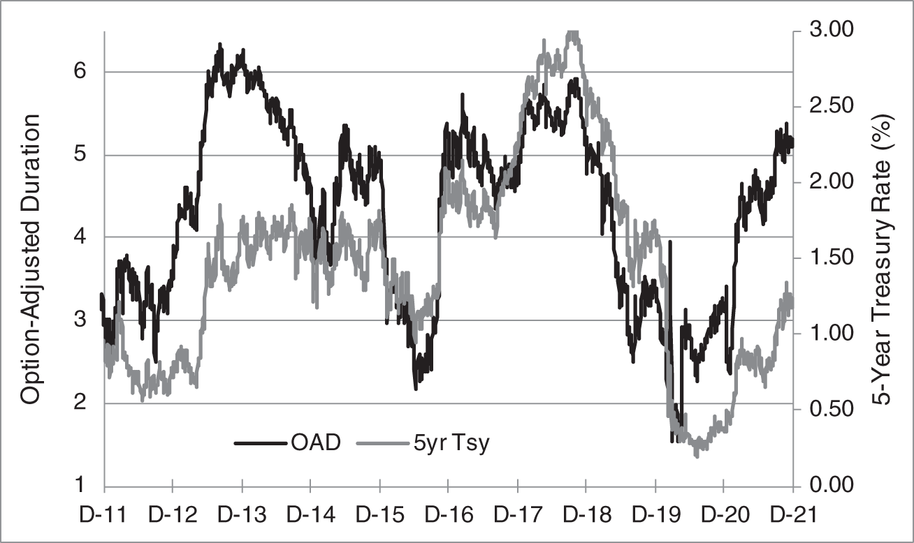
FIGURE 15.6 OAD for a FNMA 30‐Year Index and the Five‐Year Treasury Rate, December 21, 2011, to December 21, 2021.
15.8 TBA AND SPECIFIED POOLS MARKETS
The vast majority of secondary trading of pass‐through securities takes place in the very liquid TBA market, while the rest takes place in the less liquid specified pools market. The TBA market is a forward market in securitized mortgage pools, in which the seller has a delivery option. Table 15.6 shows a snapshot of TBA prices for UMBS 30‐year pools from late December 2021. The rows correspond to different delivery months, the columns correspond to different mortgage pool coupons, and the entries give the corresponding forward prices. Most of the liquidity in the TBA market is concentrated in a few coupons, although a fuller stack of coupons do trade. Most of the liquidity is also in the front or first contract and the second contract, but later delivery months trade as well. The front contract with the greatest price less than par is called the current contract. The current coupon, or current coupon rate, which is often quoted as a description of the prevailing mortgage rate, is defined as the coupon that would give a TBA contract priced at par, calculated by interpolating the coupon of the current contract and the coupon of the front‐month contract with a price just above par. From Table 15.6, the current contract is the January 2.0% TBA, and the current coupon, calculated from the coupons and prices of the January 2.0% and January 2.5% TBAs, is about 2.11%.
A seller of $1 million face amount of the January UMBS 30‐year 2.5% TBA commits to sell $1 million principal amount of a 30‐year 2.5% UMBS pool (i.e., one issued by FNMA or FHLMC) at 101–28 for settlement or delivery in January 2022. The TBA buyer commits to buy the pool delivered by the seller. The exact settlement date is published well in advance, and is always in the stated delivery month, but varies over time and by product.12 With respect to Table 15.6, the settlement dates for the three months are January 13, 2022, February 14, 2022, and March 14, 2022.
TABLE 15.6 Bid Prices for UMBS 30‐Year TBAs as of December 30, 2021.
| Coupon | 1.5% | 2.0% | 2.5% | 3.0% |
|---|---|---|---|---|
| Jan | 96−13 | 99−15+ | 101−28 | 103−13 |
| Feb | 96−08 | 99−08+ | 101−20 | 103−08+ |
| Mar | 96−03 | 99−02 | 101−12+ | 103−03+ |
Prices are given as a handle and a number of ticks or 32nds; for example, 101–12+ is a price of![]() , or 101.390625.
, or 101.390625.
The seller of a TBA has a delivery option in the sense of being able to deliver any pool that falls within the general parameters just described.13 For this purpose, a “30‐year” pool is defined as one with a remaining maturity of between 15 years and one month to 30 years and one month. The name TBA is an acronym for to be announced, and comes from the seller's option to choose the pool to be delivered after the trade date. More specifically, the seller must notify the buyer of the exact pool to be delivered on the notification date or 48‐hour day, which is two business days before the settlement date. For the contracts in the table, the notification dates are January 11, 2022, February 10, 2022, and March 10, 2022. Note, by the way, that market practitioners always say TBA, never to be announced.
Chapters 11 and 14 describe how the pricing of Treasury note and bond futures and of credit default swaps (CDS) reflect seller choices to deliver the least valuable or “cheapest‐to‐deliver” (CTD) securities. Similarly, TBA prices reflect seller choices to deliver the least valuable eligible mortgage pools, which are typically those that refinance with the greatest speed and least predictability. The analogy to Treasury futures and CDS is not perfect, however. There is typically one security that is clearly CTD into a Treasury futures or CDS contract, while many mortgage pools might be delivered into a TBA. In fact, an important part of trading in this market is forecasting the pools likely to be delivered into TBAs given the supply and characteristics of deliverable pools outstanding. In the case of the January 2.5% TBA, for example, one dealer forecasts the delivery of pools with a WAC of 3.35%, a WALA of three months, and an average loan size of $340,000. While much analysis is needed to explain the precision of this prediction, it makes sense that pools with these characteristics have less value than other 30‐year 2.5% pools: higher WACs typically prepay faster (with the credit score caveat mentioned previously); relatively new pools typically prepay faster and have more prepayment uncertainty than seasoned, somewhat burned‐out pools; and pools with high average loan balances prepay faster as well. (Note that an average loan balance of $340,000 is large relative to the averages presented in Table 15.3.)
The other secondary market for pass‐through trading is the specified pools market. Because the least valuable pools are delivered into TBAs, which is reflected in TBA prices, sellers with more valuable collateral, along with buyers wanting more valuable collateral, prefer to trade particular or specified pools. Prices of pools traded in this market are quoted as a pay‐up relative to the comparable TBA. Table 15.7 shows a sample of pay‐ups for UMBS 30‐year specified pools as of December 2021. The first four rows are pools with loan balances in particular ranges. Pools with a coupon of 2.5% and average loan balances between $125,000 and $150,000, for example, sell at a pay‐up of 37 ticks, that is, for ![]() or 1.15625 over the price of the UMBS 30‐year 2.5% front contract TBA. The pay‐ups in each of the three coupon columns decrease with average loan balance, consistent with the empirical regularity that pools with higher loan balances refinance faster. That pools with average loan balances between $200,000 and $250,000 command a pay‐up reflects the expectation, mentioned in the previous paragraph, that CTD pools have an even larger average loan balance of $340,000. For any given balance range, the pay‐up increases with coupon: relatively low loan balances and slower refinancing speeds are more valuable the higher the coupon, that is, the greater the incentive to prepay and the greater the loss in value to investors as a result of refinancings.
or 1.15625 over the price of the UMBS 30‐year 2.5% front contract TBA. The pay‐ups in each of the three coupon columns decrease with average loan balance, consistent with the empirical regularity that pools with higher loan balances refinance faster. That pools with average loan balances between $200,000 and $250,000 command a pay‐up reflects the expectation, mentioned in the previous paragraph, that CTD pools have an even larger average loan balance of $340,000. For any given balance range, the pay‐up increases with coupon: relatively low loan balances and slower refinancing speeds are more valuable the higher the coupon, that is, the greater the incentive to prepay and the greater the loss in value to investors as a result of refinancings.
TABLE 15.7 Representative Pay‐ups for Selected Specific UMBS 30‐Year Pools, in Ticks (32nds), as of December 2021.
| Coupon | |||
|---|---|---|---|
| Specified Pool Description | 2.0% | 2.5% | 3.0% |
| Average Loan Balance | |||
| Less than $85,000 | 36 | 58 | 109 |
| Between $85,000 and $110,000 | 31 | 49 | 88 |
| Between $125,000 and $150,000 | 23 | 37 | 71 |
| Between $200,000 and $225,000 | 10 | 16 | 44 |
| 100% NY Loans | 9 | 28 | 75 |
| 100% Investor Property | 3 | 14 | 34 |
| Jumbo | −14 | −18 | −38 |
The next row of Table 15.7 gives the pay‐ups for pools made up of loans in New York State, which, as mentioned earlier, refinance slowly relative to loans in other states. And, once again, those lower refinancing speeds are worth more the greater the coupon. The next row is for pools composed of loans for investor property. As discussed already, investor properties face higher refinancing rates, and, therefore, refinance more slowly, resulting in positive pay‐ups that increase with coupon.
The last row of the table gives pay‐ups for pools containing jumbo loans, that is, loans of size greater than agency conforming limits. This row differs from others in that jumbo pools are not deliverable into TBAs. In any case, jumbo pools trade at a negative pay‐up, that is, at lower prices than TBAs, because these extremely large loans are expected to prepay faster than any conforming pool delivered into TBAs.
Table 15.7 gives only a sample of specified pools. Other specified pools, with other defining characteristics, trade as well, like low FICO loans, high SATO loans, and loans serviced by certain banks. As for this last category, certain origination channels and servicing arrangements are more aggressive than others in encouraging homeowners to refinance. As a result, a pool of loans in less aggressive settings, like those serviced by certain banks, are expected to prepay more slowly and, therefore, command a pay‐up in the specified pools market.
15.9 RISK FACTORS AND HEDGING AGENCY MBS
Participants in agency MBS face and have to manage a number of risks: interest rate risk, which includes convexity and volatility risks; mortgage spread risk; prepayment risk; and credit risk. Interest rate risk is discussed extensively in earlier chapters of the book. Mortgages are clearly exposed to the risk that rates rise and fall, and, as described before, exhibit negative convexity. Furthermore, negatively convex positions are also short interest rate volatility.14
Mortgage spread risk refers to the risk of changes in the spread between mortgage rates and benchmark rates, that is, Treasury or swap rates. If an MBS is hedged by selling Treasury futures and then mortgage spreads increase, the MBS falls in value relative to the Treasury hedge and the overall position loses money. If, on the other hand, one MBS is hedged by another, perhaps a TBA, then changes in value due to mortgage spreads can offset. Prepayment risk, following earlier discussions, is the risk that prepayments are higher than anticipated for premium mortgages or lower than anticipated for discount mortgages. Finally, the credit risk from agency MBS, the risk of interest and principal loss due to homeowner default, is borne by the agencies that guarantee the underlying mortgages or the MBS.
Various groups of market participants face these risks in different permutations. Originators, who make mortgage loans in order to sell them into MBS, are exposed to pipeline risk. Originators offer firm rates to borrowers, called rate locks, but it then takes time to close or complete the mortgage deal. A possible hedge against the risk that rates rise before the mortgage can be sold is to short Treasuries or pay fixed in swaps, with hedge ratios calculated as OADs to account for prepayment risk. But this strategy has three problems. First, borrowers can walk away from rate locks at their discretion. While a deal might not close for many reasons, borrowers do tend to abandon offers when rates subsequently decline, while they tend to close on mortgages when rates subsequently increase. Accurate hedging of pipeline risk, therefore, has to account for the exercise of this borrower option. Second, because mortgages are negatively convex, hedging them with positively convex Treasuries or swaps leaves an overall negatively convex and short volatility position. One solution is to buy short‐term payer swaptions to manage convexity and to buy longer‐term swaption straddles to hedge the volatility.15 Third, because mortgage values and this borrower option depend on prevailing mortgage rates, rather than on Treasury or swap rates, hedges with Treasuries or swaps are subject to mortgage spread risk.
An alternative hedge of originator pipeline risk is to sell TBAs rather than Treasuries or swaps. Prepayment models are still needed to calculate hedge ratios, and the problem of modeling rate‐lock optionality remain. But because TBAs are also negatively convex and short volatility, selling them can offset the negative convexity and short volatility properties of the mortgages being originated. In that case, swaptions are necessary only to address any residual exposures. Furthermore, because both TBAs and the mortgages being originated clearly depend on mortgage spreads, that risk can be mitigated by the TBA hedge as well.
Originators that hedge pipeline risk by selling TBAs have another decision to make when the originated pools are ready for sale. If the pools are significantly more valuable than TBA prices, the originator can buy back the TBA hedge and sell the pools in the specified pool market. If the pools are about as valuable as TBA prices, the originator can deliver the pools into the short TBA hedges. And if the pools are worth somewhat more than TBA prices, there is a trade‐off of value and liquidity: the pools may be worth somewhat more if sold as specified pools, but they can be sold with more liquidity in the TBA market.16
Mortgage servicers lose revenue when mortgage rates decline and homeowners refinance. This effect tends to dominate the increase in value of the remaining servicing flows due to discounting at lower rates. Mortgage servicing rights, therefore, usually have significant negative duration. They are also negatively convex. Their interest rate sensitivity increases as rates increase: from very negative at low rates, when homeowners are prepaying fast, to less negative at high rates, when homeowners are prepaying slowly. One possible hedge of servicing revenue is to buy Treasuries or receive fixed in swaps. The determination of hedge ratios requires a prepayment model, of course, but the resulting, overall position is negatively convex, short volatility, and subject to mortgage spread risk. The alternative of hedging by buying TBAs is not as appealing a solution as it is for originators. True, buying TBAs across the stack of coupons can increase the effectiveness of prepayment hedging. And true, buying TBAs against servicing rights hedges mortgage spread risk. But with both mortgage servicing rights and long TBA positions negatively convex and short volatility, the overall “hedged” position is even more negatively convex and short volatility. If that result is unacceptable from a risk management perspective, swaptions can be bought – at a cost – to flatten out the exposure.
As mentioned earlier in the chapter, some servicers are also originators, and servicing and origination businesses, at least to some extent, hedge each other. It might be cheapest, at least in theory, for entities with both businesses to rely on this operational hedge and hedge only residual risk with Treasuries or swaps, TBAs, and swaptions. In practice, however, organizational efficiencies might lead each business to hedge its risk independently. In that case, a middle ground might be to save on transaction costs by crossing hedging trades internally.
The various market participants that invest in mortgages can decide which risks to bear and which risks to hedge. A mortgage exchange‐traded fund is likely to buy MBS and take all of the associated risks, in the expectation of earning commensurate return. A more actively managed mortgage portfolio might hedge out interest rate risk with Treasuries or swaps, and even negative convexity and volatility with swaptions, but keep mortgage spread risk and prepayment risk, possibly to earn appropriate compensation for bearing those risks over time, or possibly to take advantage of perceived skill in timing exposures to those risks. Finally, a relative value mortgage desk might bet on prepayment speeds alone, essentially depending on its prepayment model outperforming the market consensus and implied pricing. This strategy is most likely implemented by buying relatively cheap specified pools and selling relatively rich TBAs, or vice versa, or by trading one TBA coupon against another in the stack.
Last but not least are the agencies. They manage the default risk arising from their guarantees in two ways. First, they collect g‐fees that are designed to be sufficient, in aggregate, to make up for experienced losses. Second, agencies sell off some of their default risk to the private sector through credit risk transfer securities, which are discussed presently. The extent to which the agencies bear other mortgage risks depends on the method by which the MBS are issued. In lender swap transactions, which are the most common, an agency exchanges mortgage loans from originators for MBS made up of those loans. The loans move directly into a trust backing the MBS without ever residing on the agency's balance sheet. Therefore, in this kind of issuance, all risks (other than default) remain with the originator. In portfolio securitization transactions, by contrast, an agency buys mortgages for its own portfolio, packages them into MBS, and sells those MBS in the secondary market. In this method of issuance, the agency bears interest rate risk, prepayment risk, and mortgage spread risk from the time the mortgages are purchased until the time they are sold through MBS. Along the lines of the earlier discussion about private originators, an agency can hedge these risks by selling Treasuries or swaps, or by selling TBAs, and by supplementing these hedges with the purchases of swaptions. Also, like other originators, agencies can decide whether to buy back TBA hedges and sell originated pools in the specified pools market or to deliver originated pools into their short TBA hedges.
This section concludes with a further observation about the TBA and specified pools markets. On the one hand, the TBA delivery option means that TBA prices track those of the least valuable pools. But on the other hand, from a primary market that produces a huge number of distinct pools, the TBA delivery option creates extremely liquid secondary market trading in a handful of TBA contracts. This liquidity allows market participants to hedge their specified pool exposures with TBAs; that is, the liquidity of the TBA market easily compensates for any basis risk arising from differences between changes in specified pool prices and changes in TBA prices. Furthermore, the liquidity of the TBA market is so attractive that many pools are, in fact, physically delivered – and thus sold – through TBA contracts, despite relatively low TBA prices due to the delivery option, and despite the general preference of derivatives users to unwind derivatives hedges and to trade physical or cash product with their regular business counterparties.
15.10 DOLLAR ROLLS
Because TBA liquidity is concentrated in contracts that mature in one of the next several months, market participants often need to roll their positions in maturing contracts to contracts that mature at later dates. For example, originators and investors that are short January 2022 TBAs to hedge exposures but wish to keep those short positions past the January settlement date, can buy the roll, that is, buy (back) the front month contract (January) and sell contracts expiring in later months, perhaps in February. Similarly, servicers and investors who are long January 2022 TBAs, but wish to maintain those longs past January, can sell the roll, that is, sell (out of) the front month contract (January) and buy contracts expiring in later months. These TBA rolls are also called dollar rolls.
A natural question that arises in the context of dollar rolls is whether TBA prices are fair relative to one another. Because TBAs are forward contracts, several of the insights of Chapters 10 and 11 apply here. First, a long TBA position is similar to a long position in the underlying pool and a short repo position (i.e., borrowing money on the collateral of the pool). Second, TBA prices will exhibit forward drops so long as the carry on the pool exceeds the repo rate. This is illustrated, in fact, in Table 15.6. The repo rate at the time is 10 basis points; all the TBA coupons shown significantly exceed that repo rate; and TBA prices are lower for later expiration months. Third, just as each TBA has implicit financing from the trade date to settlement, a TBA roll embeds implicit financing from the expiration of the front contract to the expiration of the deferred contract.
Market practitioners calculate the value of a roll and the implied financing rate or breakeven financing rate of a roll along the lines of the cash‐and‐carry arbitrage for forward contracts on coupon bonds discussed in Chapter 11. In that context, however, the forward contract is on a particular bond and that bond's coupon is known with certainty. In the TBA context, because of the delivery option, the forward contract is on an unknown pool. Furthermore, because of prepayments, the cash flows of pools are not known with certainty. An industry standard roll analysis puts these issues aside, essentially assuming that rolls are perfectly equivalent to mortgage repo. After presenting this analysis, the text returns to the differences between TBA and repo financing.
Consider an investor who holds $1,000,000 of a 30‐year 2.5% pool in early January 2022. Assume that TBA prices are as in Table 15.6 and that the mortgage repo rate of 10 basis points is the relevant risk‐free rate. Also, consistent with the discussion in the previous paragraph, assume for the purposes of this analysis that the February cash flow from the pool (payable to investors on February 25) is known and equal to $10,850.00, which includes $8,800.00 of principal (both scheduled payments and prepayments).
The investor holding the pool is considering two strategies, both of which leave the investor with the same outstanding balance of the pool on 2/14: i) hold the pool to February 14, the settlement date of the February TBA, at which point the principal outstanding balance is $1,000,000 minus $8,800.00, or $991,200; ii) sell the pool through the January TBA for 101–28 (101.875) and buy back $991,200 of the pool through the February TBA at 101‐20 (101.625). The assumption that the investor will get back the same pool that had been sold in January is again consistent with the simplifications of this analysis. Figure 15.7 summarizes these two strategies: holding the pool, below the line, and ii) rolling, above the line.
The cash flows from holding the pool are very simple. The February payment of $10,850.00 is received on 2/25, but, for comparison purposes, is discounted 11 days, back to 2/14, for a present value of ![]() .
.
The cash flows from rolling are as follows. The pool is sold through the January TBA for flat proceeds of ![]() , plus 12 days of accrued interest, that is,
, plus 12 days of accrued interest, that is, ![]() , for total proceeds of $1,019,583.33. These proceeds are invested at the repo rate from 1/13 to 2/14, that is, for 32 days, to earn interest of
, for total proceeds of $1,019,583.33. These proceeds are invested at the repo rate from 1/13 to 2/14, that is, for 32 days, to earn interest of ![]() . The next part of this strategy is to buy $991,200.00 face amount of the pool through the February TBA at a flat cost of
. The next part of this strategy is to buy $991,200.00 face amount of the pool through the February TBA at a flat cost of ![]() , plus accrued interest of 13 days of
, plus accrued interest of 13 days of ![]() , for a total cost of $1,008,201.83. Finally, subtracting this cost from the invested proceeds of the January sale leaves a net of $11,472.13.
, for a total cost of $1,008,201.83. Finally, subtracting this cost from the invested proceeds of the January sale leaves a net of $11,472.13.
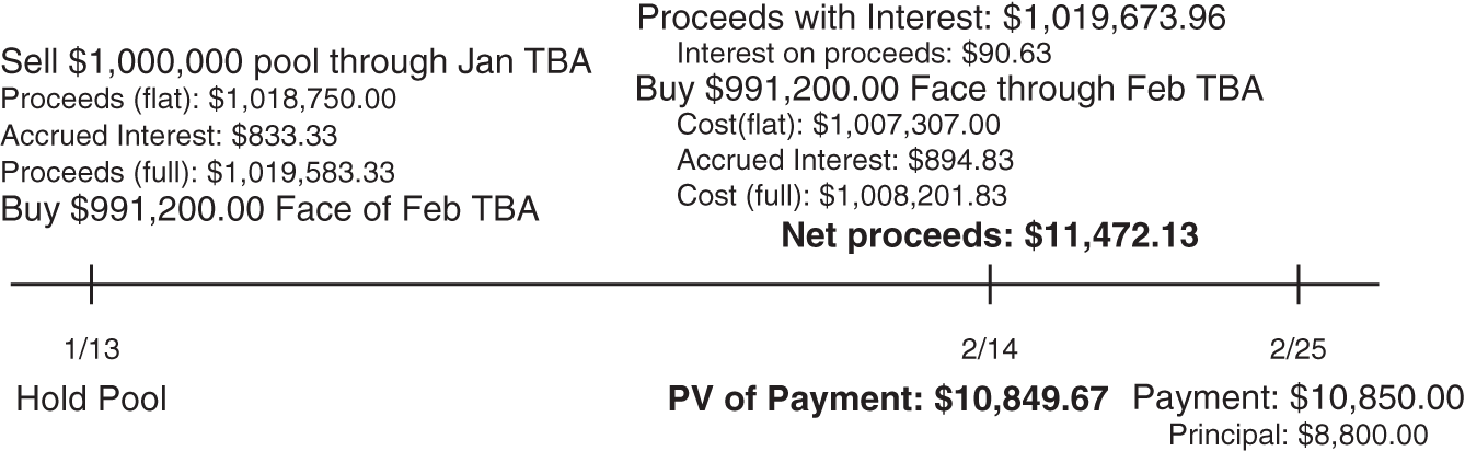
FIGURE 15.7 Dollar Roll Example, UMBS 30‐Year 2.5% Jan−Feb TBAs, as of January 2022.
Putting the pieces together, both the hold and roll strategies leave the investor with $991,200 of the pools as of 2/14. But the roll strategy also leaves the investor with net proceeds of $11,472.13 on 2/14, while the hold strategy leaves the investor with $10,849.67. The value of the roll, defined as the difference between these two amounts, is $622.46. Hence, according to this analysis, the January TBA is rich relative to the February TBA, or, in other words, investors are willing to pay up to have the 2.5% pools now.
The advantage of the roll is often expressed as an implied or breakeven financing rate, which, replacing the repo rate, sets the value of the roll to zero. In this example, the implied financing rate is ![]() 58.4 basis points. The difference between the actual repo rate of 10 basis points and this implied rate, or about 68 basis points, is known as the specialness of the pools. From a rates perspective, owners of the 2.5% pools can earn 68 basis points over repo by giving up their pools for a month.
58.4 basis points. The difference between the actual repo rate of 10 basis points and this implied rate, or about 68 basis points, is known as the specialness of the pools. From a rates perspective, owners of the 2.5% pools can earn 68 basis points over repo by giving up their pools for a month.
While the numbers in this example are rounded for easy reading, the implied financing rate of ![]() 58 basis points is consistent with the analysis circulated by market professionals at the time. The discussion circles back then, to the simplifying assumptions behind the standard dollar roll analysis. First, the assumption that the same pool will be returned to the owner in February overstates the desirability of the roll to the owner of the pool: the TBA delivery option opens the roll seller to the risk of receiving a pool of lower value. Second, the prepayment assumption is critical in the calculation of the breakeven rate. Slower prepayments make holding the pool more valuable, or equivalently, reduce the value of the roll and increase the implied financing rate. Third, the assumption of known prepayments overstates the desirability of holding the pool, or equivalently, understates the value of the roll, because prepayments are, in fact, uncertain, and prepayment risk is borne by the holder of the pool.
58 basis points is consistent with the analysis circulated by market professionals at the time. The discussion circles back then, to the simplifying assumptions behind the standard dollar roll analysis. First, the assumption that the same pool will be returned to the owner in February overstates the desirability of the roll to the owner of the pool: the TBA delivery option opens the roll seller to the risk of receiving a pool of lower value. Second, the prepayment assumption is critical in the calculation of the breakeven rate. Slower prepayments make holding the pool more valuable, or equivalently, reduce the value of the roll and increase the implied financing rate. Third, the assumption of known prepayments overstates the desirability of holding the pool, or equivalently, understates the value of the roll, because prepayments are, in fact, uncertain, and prepayment risk is borne by the holder of the pool.
In summary, financing in the mortgage market is available directly, through repo, and indirectly, through TBAs. The liquidity of the TBA market is a factor in its favor. Repo financing keeps the prepayment risk of intermediate payments with the owner of the collateral, while TBA positions avoid that risk. Repo financing keeps control of the collateral; long TBA positions give up control of collateral; and short TBA positions are long a delivery option.
15.11 OTHER MBS
This section briefly describes MBS other than individual pools. As mentioned earlier, because pass‐through securities are relatively large, diversified, and insured portfolios of mortgages, they are owned by a broader investor base and trade with more liquidity than individual mortgages. Taking this another step, the agencies combine pools into larger MBS, to create even more diversified and, if successful, more liquid securities. These conglomerated MBS with FNMA collateral are called Megas; with FHLMC collateral, Giants; and with collateral from both agencies, Supers.
Another type of MBS of significant size are REMICs (Real Estate Mortgage Investment Conduits) or CMOs (Collateralized Mortgage Obligations). While pass‐through MBS have proved popular with many investors, others are less comfortable with prepayment risk, that is, with securities whose duration can fluctuate widely, as illustrated in Figure 15.6. Some CMO and REMIC classes or tranches address this problem. SEQs (sequential pay classes), for example, are structured as follows. The cash flows from an underlying portfolio of pools are passed through to a number of distinct SEQ classes. All classes receive monthly interest payments, but principal payments from the underlying pools are directed first to pay off the A class. Once the principal amount of the A class is fully paid off, principal payments from the pools are directed to the B class, and so forth. While SEQ classes still bear significant prepayment risk, their effective maturities can be bucketed with somewhat more granularity than standard pass‐through MBS.
PACs, or planned amortization classes, are further along in the spectrum of creating more complicated structures so as to create some securities with less prepayment risk. Once again, the cash flows of an underlying portfolio of pools are divided across a number of classes. PAC classes, however, promise fixed schedules of principal payments so long as prepayment rates stay within set ranges. Making this possible are support or companion classes that absorb prepayment fluctuations within these ranges. If prepayments are relatively fast, then the support classes get paid principal quickly, enabling the PAC classes to maintain their fixed payment schedule. Conversely, if prepayments are relatively slow, the support classes absorb the shock by being paid principal particularly slowly. If prepayment rates move outside the set ranges, however, the PAC bonds will experience faster or slower principal payments as well. Similar to PACs are TACs (targeted amortization classes), which protect only against faster prepayments, and which are usually included in structures that include PACs as well. The issuance of CMOs offering PACs and TACs is viable, because their classes can be sold for more than the underlying pools. In other words, some investors are willing to pay up enough for MBS with prepayment protection so as to more than compensate the investors who buy and take on the amplified risks of the support classes.
Interest‐only (IO) and principal‐only (PO) strips are another well‐known set of MBS products. The cash flows of an underlying portfolio of pools are directed into these two classes by a simple rule: all interest payments are paid to the IOs and all principal payments to the POs. The price sensitivities of these strips are larger than many other fixed income products. As rates fall and prepayments increase, the cash flows of the IOs begin to vanish. This loss of value more than offsets any gains from higher discount factors on remaining cash flows, and IO prices decline. Hence IOs, like mortgage servicing rights, have negative durations at low levels of rates. Conversely, POs gain dramatically in value as rates decline. They have the relatively high interest rate sensitivity of zero coupon bonds, with the added effect of early repayment of principal when rates are low.
15.12 CREDIT RISK TRANSFER SECURITIES
One reform following the 2008 government rescue of the GSEs was to have the GSEs sell some of the mortgage default risk from their MBS guarantees to the private sector. To this end, GSEs started to offer credit risk transfer (CRT) securities to the public in 2013, called Connecticut Avenue Securities (CAS) at FNMA and Structural Agency Credit Risk (STACR) securities at FHLMC.17 The basic idea is that investors buy bonds at par; earn a spread over a short‐term rate; and, in exchange for that spread, bear some of the default risk on a reference pool of mortgages. More specifically, as defaults on that pool reach certain thresholds, investors lose some or even all of the principal on their bonds. A somewhat simplified explanation of how CRTs work is presented in this section, with reference to a recent offering, CAS 2020‐R01, summarized in Table 15.8. The notes actually offered to the public through CAS 2020‐R01 are highlighted in bold, namely, the M1, M2, and B1 classes. The A and B2 classes, along with the M1, M2, and B1 amounts in the FNMA column, are fictional: they are included in the description of CRTs only to explain how the cash flows of the actual notes are determined.
TABLE 15.8 Connecticut Avenue Securities (CAS) 2020‐R01, Issued in January 2020 and Maturing in January 2040. Spread Is Over One‐month LIBOR.
| Reference‐Pool Balance ($mm): | 28,996 | |||||
|---|---|---|---|---|---|---|
| Class | Notes | FNMA | Credit Support | Thickness | Rating | Spread |
| ($mm) | ($mm) | (%) | (%) | (Fitch) | (bps) | |
| A | 27,851 | 3.95 | ||||
| M1 | 303 | 16 | 2.85 | 1.10 | BBB‐ | 80 |
| M2 | 523 | 28 | 0.95 | 1.90 | B | 205 |
| B1 | 207 | 11 | 0.20 | 0.75 | NR | 325 |
| B2 | 58 | 0.00 | 0.20 | |||
| Total | 1,033 | |||||
The first step in creating a CRT is to select a group of mortgage loans for inclusion in the reference pool. All candidate loans are conforming but are further scrutinized to exclude those with “underwriting defects” and “performance deficiencies.” This screening is one of several ways the GSEs seek to assure CRT investors that they are taking representative mortgage default risk, rather than default risk of a particularly weak group of loans. In any case, the reference pool chosen for CAS 2020‐R01, at the time of issue, had over 100,000 loans and a total balance of about $29 billion.
At issuance, investors buy a total of $1.033 billion principal amount of notes at par, $303 million in the M1 class, $523 million in the M2 class, and $207 million in the B1 class. The proceeds from this sale are deposited into a trust that earns enough to pay investors a short‐term rate on their principal, here one‐month LIBOR. In addition, the GSE commits to contribute some of the g‐fees it earns to pay the CRT investors a spread over that short‐term rate, in particular, 80, 205, and 325 basis points on the M1, M2, and B1 classes, respectively. In exchange for that spread, the investors bear some of the default risk of the reference pool of mortgages, in a manner to be described presently.
The return of principal to CRT noteholders depends on the principal cash flows of the reference pool. It is important to emphasize, however, that cash flows from the reference pool do not, in any sense, flow to CRT investors. The owner of each loan in the reference pool, whether a GSE or some MBS investor, receives all of the interest and principal cash flows from that loan. The interest and principal paid to CRT investors comes from the CRT trust, with the interest supplemented by the GSE contributions mentioned in the previous paragraph.
As the reference pool makes voluntary principal payments (i.e., scheduled principal payments and prepayments that are not due to default), principal is returned to the CRT notes. The A or senior class receives principal in proportion to its outstanding balance relative to the remaining balance of the reference pool. At issuance, for example, the A class is $27,851/$28,996, or about 96% of the outstanding reference‐pool balance. Therefore, the A class is allocated 96% of the voluntary principal payments from the reference pool. Of course, as mentioned earlier, the A class does not really exist, and is just used for calculating cash flows due to the actual notes. But, along those lines, the principal balance of the A class is reduced by these fictional returns of principal. The remainder of principal payments from the reference pool, or about 4% at the time of issuance, is allocated to the M1, M2, B1, and B2 or subordinate classes, in order of seniority. This means that, so long as the M1 class has an outstanding principal balance, all of the principal payments to the subordinate classes are allocated to M1. When the M1 notes are completely paid off, these principal payments are allocated to M2 and so on. Note that the principal payments to the M1, M2, and B1 classes are real. The calculation of the payments are as described, based on the principal payments of the reference pool, but the payments themselves come from the CRT trust into which the original sale proceeds were deposited.
The text now turns to the crux of the structure, namely, the allocation of default losses in the reference pool to CRT note investors. Once again, to assure CRT investors, the issuing agency holds the first‐loss tranche, which, for CAS 2020‐R01, is the fictional B2 class. According to Table 15.8, FNMA held $58 million of this class, which is assigned losses starting from a credit support of 0% to a total thickness of 0.20% of the original $28.996 billion reference‐pool balance, which is also $58 million.18 If the reference pool suffers $1 million of losses, the principal of the B2 class falls from its original $58 million to $57 million. If the pool experiences another $5 million of losses, another $5 million of B2 principal is written down, to $52 million, and so forth. If cumulative losses ever reach $58 million, the B2 class is written down to zero.19
If losses are large enough to burn through the first‐loss tranche, the real CRT investors start to lose principal. According to Table 15.8, the original principal of the B1 class was $218 million, of which 95% or $207 million was held by private investors, and 5% or $11 million was assigned to FNMA. FNMA holds 5% of the B1 class, as well as 5% of the M1 and M2 classes, as “skin‐in‐the‐game,” to assure investors of each class that their interests and FNMAs are aligned. These 5% holdings of each class are examples of vertical slices, because they are treated just as investor holdings in the same class. Horizontal slices, by contrast, are treated better or worse than other classes, like the B2 and A classes.
With credit support of 0.2%, B1 does not suffer any principal write‐downs until reference‐pool losses exceed 0.2% or $58 million, or, equivalently, until the B2 class has been wiped out. Any further losses, however, are for the most part borne by B1 noteholders. If the reference pool experiences $1 million of losses beyond $58 million, 95% of those losses or $950,000 result in a write‐down of B1 principal from the original $207 million to $206,050,000, and 5% or $50,000 of those losses result in a write‐down of FNMA's fictional B1 principal from $11 million to $10,950,000. Operationally, the CRT trust sends $950,000 to FNMA, which uses those funds either to compensate MBS investors, or, if the loans are held in its own portfolio, to avoid suffering losses on its own account.
The B1 class is wiped out itself if losses beyond $58 million equal the class thickness of 0.75% of the original reference pool, that is, 0.75% times $28.996 billion, or $218 million. In that case, further losses hit first the M2 and then the M1 classes, in the same way as just described for the more junior classes. All in all, FNMA's B2 class bears the first 0.2% of losses; the B1, M2, and M1 classes bear the next 3.75% of losses, with $1.033 billion borne by private investors and $55 million by FNMA; and any further losses are retained by FNMA. With long‐term, historical losses rarely exceeding 4.00%, this structure, which resembles that of most other CRTs, is designed to protect FNMA against losses other than those from its first‐loss class and its skin‐in‐the‐game vertical slices.
Finally, circle back to the relative ratings and spreads of the various CRT classes in Table 15.8. The more junior the class, the more exposed the principal to loss, the lower the rating, and the higher the spread. CRTs are bought mostly by money managers and hedge funds, with money managers favoring the more senior and hedge funds the more junior classes. Across some recent issues, about 80% to 95% of M1 classes were bought by money managers, and between about 60% and 75% of B2 classes were bought by hedge funds.20
The pandemic and economic shutdowns starting in 2020, bringing heightened concerns about homeowner defaults and the effects of forbearance programs, have challenged the CRT market. Both GSEs, in fact, stopped issuance for a time, but FHLMC re‐entered the market in summer 2020, as did FNMA in the last quarter of 2021.
NOTES
- 1 For a concise history, see, for example, Federal Housing Finance Agency (2011), “A Brief History of the Housing Government‐Sponsored Enterprises,” in Inaugural Semiannual Report to the Congress, March 31, pp. 47–54.
- 2 The establishment of the conservatorship itself did trigger a credit default swap auction on GSE debt, and final auction prices were less than par. Nevertheless, bonds issued by the GSE made timely payments of all interest and principal.
- 3 “Gross” issuance includes refinancings. But because refinancings extinguish existing mortgages, they do not necessarily add to net outstanding mortgage principal. In a first‐lien mortgage, the lender has first or senior rights to the property. A homeowner's primary mortgage is a first lien, while any additional loans taken on the same property, like loans to make the required down payment and home equity loans, are second liens and junior to the first lien.
- 4 FICO is a credit metric created by the Fair Isaac Corporation that increases with measured borrower creditworthiness, to a maximum of 850. DTI is defined as monthly debt payments divided by monthly income.
- 5 Jumbo loans were between 3% and 4% of all loans from 2018 through the first half of 2020. See Federal Housing Finance Agency (2021), “What Types of Mortgages Do Fannie Mae and Freddie Mac Acquire?” April 14, pp. 2–3.
- 6 See Fritzdixon, K. (2019), “Bank and Nonbank Lending over the Past 70 Years,” FDIC Quarterly 13(4), pp. 31–39; and Ginnie Mae (2021), “Global Markets Analysis Report,” December, p. 26.
- 7 Federal Housing Finance Agency (2021),“What Types of Mortgages Do Fannie Mae and Freddie Mac Acquire?” April 14.
- 8 The rest of this chapter ignores this payment delay, but practitioners do account for it, of course, when pricing MBS.
- 9 By way of illustration, the WAMs and WALA of CA2797 can conceivably be reproduced as follows. Say that, at issue, the pool has 90% of its balance in new loans maturing in 361 months and 10% of its balance in new loans – perhaps used for refinancing – maturing in 351 months. Then assume that, by the report date, all of the 361‐month loans prepaid and none of the 351‐month loans prepaid. That would leave, as of the report date, a pool with a WAM of
 and a WALA of 37.
 - 10 In the excluded period, mortgage prices fell dramatically – and their OAS relative to Treasuries increased dramatically – because of market stress and increased volatility rather than because of changes in the level of interest rates.
- 11 As explained in Chapter 4, duration is computed using smaller rate perturbations, but quoted in units that correspond to a percentage change in price for a 100‐basis‐point decrease in rate.
- 12 “Class A” settlement dates apply to 30‐year UMBS TBAs; “Class B” to 15‐year UMBS and GNMA; “Class C” to 30‐year GNMA; and “Class D” to an assortment of other products.
- 13 Some TBA trades include stipulations or stips that add restrictions on deliverable pools.
- 14 The discussions about interest rate risk in this section rely heavily on the material about convexity from Chapter 4 and material about swaptions in Chapter 16.
- 15 Swaptions are discussed in Chapter 16. Like any option, a swaption has a positively convex price–rate profile, which can be used to manage the convexity of other positions. Also, like any options, swaptions increase in value with volatility. Shorter‐term swaptions, however, are less exposed to volatility than long‐term options.
- 16 An originator can also sell pools into other securitizations, like CMOs, discussed in a later section.
- 17 The GSEs have additional programs, not discussed in the text, through which they sell off default risk to insurance companies, called credit insurance risk transfer (CIRT) at FNMA and agency credit insurance structure (ACIS) at FHLMC.
- 18 The assignment of losses in CRTs is similar to that of collateralized loan obligations, described in Chapter 14, but the nomenclature is different. The “attachment point” of CLOs corresponds to the credit support percentage here, and the “detachment point” of CLOs equals the sum of the credit support and thickness percentages here.
- 19 The text abstracts from the fact that recoveries in the event of default are uncertain. Therefore, losses assigned to tranches can be subsequently reversed if recoveries are greater than anticipated.
- 20 Freddie Mac (2021), “Credit Risk Transfer Handbook,” October, p. 23.