
APPENDIX TO CHAPTER 16
Fixed Income Options
A16.1 THEORETICAL FOUNDATIONS FOR APPLYING BLACK‐SCHOLES‐MERTON (BSM) TO SELECTED FIXED INCOME OPTIONS
The justification for applying BSM in each of the cases of the text takes the following form:
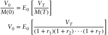
- Given the functional form of a probability distribution (e.g., normal, lognormal), there exist parameters of that distribution such that
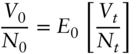
 , the arbitrage‐free price of any asset today, is given by,
where
, the arbitrage‐free price of any asset today, is given by,
where  is the price at time
  of an asset chosen as the numeraire;
  is value at time
  of an asset being priced today, including reinvested cash flows; and
  gives expectations as of time
  under the appropriately parameterized probability distribution. Equation (A16.1) is known as the martingale property of asset prices. This claim is proved in a special case in Section A16.2 but used more generally here.
 - Say that the rate or security price underlying an option at time
 is
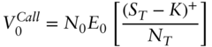
is  . It follows from the previous point that the value of a call option with strike
  and time to expiry
  is,
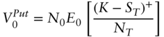
while the value of a put is,
is,
while the value of a put is,
- In the contexts of the text, it is possible to choose the numeraire such that,
and such that Equations (A16.2) and (A16.3) can be written as, respectively,
(A16.5)for some
 that is known as of time 0. This is proven in Section A16.3.
 - If
 has a normal distribution with volatility parameter
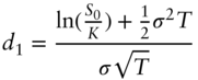
  , then Section A16.4 shows that (A16.4) through (A16.6) become the normal BSM‐style formulae,
(A16.7)
, then Section A16.4 shows that (A16.4) through (A16.6) become the normal BSM‐style formulae,
(A16.7) (A16.8)for the functions
 and
and  defined in that section. On the other hand, if
  has a lognormal distribution with volatility parameter
  , Section A16.4 shows that (A16.4) through (A16.6) become the lognormal BSM‐style formulae,
(A16.9)and
, Section A16.4 shows that (A16.4) through (A16.6) become the lognormal BSM‐style formulae,
(A16.9)and (A16.10)for the functions
 and
and  defined in that section.
A16.2 NUMERAIRES, PRICING MEASURES, AND THE MARTINGALE PROPERTY
Define the following:
- Gains process. The gains process of an asset at any time equals the value of that asset at that time plus the value of all its cash flows reinvested to that time. For this purpose, all cash flows are reinvested and then rolled at prevailing short‐term interest rates.
- Numeraire asset. Given a particular numeraire asset, the gains process of any other asset can be expressed in terms of the numeraire asset by dividing that gains process by the gains process of the numeraire asset. The gains process of a security in terms of the numeraire asset is called the normalized gains process of that asset.
For concreteness, Table A16.1 gives an example of these concepts. The asset under consideration is a long‐term, 4% coupon bond with a face amount of 100. The numeraire is a two‐year zero coupon bond with a unit face amount. The gains process is observed today, after one year, and after two years.
The realization of the short‐term rate, which in this example is the one‐year rate, is given in row (i). The realization of the bond price over time is given in row (ii). A 4% coupon on 100 is paid on dates 1 and 2 and shown in row (iii) and row (iv). The payment on date 1 is reinvested for one year at the short‐term rate on date 1, that is, 2%. The gains process of the bond given in row (v) is the sum of its price and reinvested cash flows, i.e., the sums of rows (ii) through (iv). The price realization of the two‐year zero coupon bond, which is the chose numeraire, is given in row (vi). Finally, the normalized bond gains process, given in row (vii), is the bond gains process divided by the price of the numeraire, i.e., row (v) divided by row (vi).
These definitions allow for the statement of the main result of this section: in the absence of arbitrage opportunities, there exists a parameterization of a given probability distribution, or a pricing measure, such that the normalized gains of any asset today equals the expected value of that asset's normalized gains in the future. Technically, there exist probabilities such that the normalized gains process is a martingale. As the goal here is intuition rather than mathematical generality, this result is proven in the context of a single‐period, binomial process.
TABLE A16.1 Example of the Calculation of a Normalized Gains Process
| End‐of‐Year Realizations | ||||
|---|---|---|---|---|
| 0 | 1 | 2 | ||
| (i) | Short‐Term/1‐Year Rate | 1% | 2% | 1.5% |
| (ii) | Bond Price | 100 | 95 | 97.50 |
| (iii) | Date 1 Reinvested Coupon | 4 | 4(1.02)=4.08 | |
| (iv) | Date 2 Reinvested Coupon | 4 | ||
| (v) | Gains Process | 100 | 99 | 105.58 |
| (vi) | Price of 2‐Year Zero/Numeraire | 0.9612 | 0.9804 | 1.0 |
| (vii) | Normalized Bond Gains Process | 104.04 | 100.98 | 105.58 |
The starting point is state 0 of date 0, after which the economy moves to either state 0 or state 1 of date 1. Three assets will be considered, A, B, and C, with current prices ![]() ,
, ![]() , and
, and ![]() , and date 1, state
, and date 1, state ![]() prices of
prices of ![]() ,
, ![]() , and
, and ![]() . Without loss of generality here, the date 1 prices include any cash flows of the securities on date 1.
. Without loss of generality here, the date 1 prices include any cash flows of the securities on date 1.
In this framework, any asset can be priced by arbitrage relative to the other two assets. The method is just as in Chapter 7. To price asset C by arbitrage, construct its replicating portfolio, in particular, a portfolio with ![]() of asset A and
of asset A and ![]() of asset B such that,
of asset B such that,
Then, to rule out risk‐free arbitrage opportunities, it must be the case that,
Now let asset A be the numeraire and rewrite equations (A16.11) through (A16.13) in terms of the normalized gains processes of assets B and C. To do this, simply divide each of the equations by the corresponding value of the numeraire asset A, that is, divide (A16.11) by ![]() , (A16.12) by
, (A16.12) by ![]() , and (A16.13) by
, and (A16.13) by ![]() . Furthermore, denote the normalized gains process of the assets by
. Furthermore, denote the normalized gains process of the assets by ![]() and
and ![]() . Then, equations (A16.11) through (A16.13) become,
. Then, equations (A16.11) through (A16.13) become,
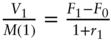
Furthermore, solving (A16.14) and (A16.15) for ![]() and
and ![]() ,
,
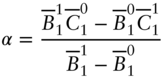
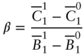
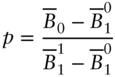
In the framework just described, it is now shown that there exists a pricing measure such that the expected normalized gains process of each security is a martingale. More specifically, there is a probability ![]() of moving to state 1 of date 1 (and
of moving to state 1 of date 1 (and ![]() of moving to state 0 of date 1) such that the expected value of the normalized gain of each security on date 1 equals its normalized gain on date 0. Mathematically, it has to be shown that there is a
of moving to state 0 of date 1) such that the expected value of the normalized gain of each security on date 1 equals its normalized gain on date 0. Mathematically, it has to be shown that there is a ![]() such that,
such that,
Solving (A16.20) for ![]() gives,
gives,
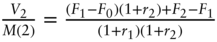
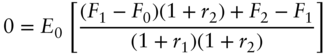
But this value of ![]() also solves (A16.19). To see this, start by substituting
also solves (A16.19). To see this, start by substituting ![]() from (A16.21) into the right‐hand side of (A16.19),
from (A16.21) into the right‐hand side of (A16.19),
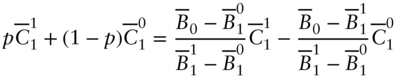
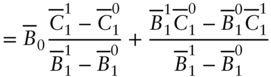
Equation (A16.23) just rearranges the terms of (A16.22); combining (A16.23) with (A16.17) and (A16.18) gives (A16.24); and (A16.24) with (A16.16) gives (A16.25). Hence, as was to be shown, there is a pricing measure, in this case the probability ![]() , such that the normalized gains processes of B and C are martingales. And, of course, since nothing distinguishes A from the other assets, a probability with the same properties could have been found had B or C been chosen as the numeraire instead.
, such that the normalized gains processes of B and C are martingales. And, of course, since nothing distinguishes A from the other assets, a probability with the same properties could have been found had B or C been chosen as the numeraire instead.
A16.3 CHOOSING THE NUMERAIRE AND BSM PRICING
In the contexts of this chapter, it is possible to choose a numeraire such that the underlying is a martingale and such that the value of a call is given by ![]() or
or ![]() , in the normal or lognormal cases, respectively, and the value of a put by
, in the normal or lognormal cases, respectively, and the value of a put by ![]() or
or ![]() in the normal or lognormal cases, where those functions are defined in Section A16.4. This section gives the appropriate definition of the underlying, the appropriate numeraire, and the resulting quantity
in the normal or lognormal cases, where those functions are defined in Section A16.4. This section gives the appropriate definition of the underlying, the appropriate numeraire, and the resulting quantity ![]() .
.
A16.3.1 Bond Options
Start with a European‐style option, expiring on date ![]() , written on a longer‐term bond. The underlying of this option is a forward position in the bond for delivery on date
, written on a longer‐term bond. The underlying of this option is a forward position in the bond for delivery on date ![]() . It is first shown that taking the zero coupon bond maturing at time
. It is first shown that taking the zero coupon bond maturing at time ![]() to be the numeraire makes this forward bond price a martingale. Proving this is somewhat complex, because the gains process of a bond includes reinvested coupons. Therefore, to keep the presentation simple, the martingale result is derived in a three‐date, two‐period setting. The current date is date 0, and the expiration or forward delivery date is date 2. The bond is assumed to pay a coupon
to be the numeraire makes this forward bond price a martingale. Proving this is somewhat complex, because the gains process of a bond includes reinvested coupons. Therefore, to keep the presentation simple, the martingale result is derived in a three‐date, two‐period setting. The current date is date 0, and the expiration or forward delivery date is date 2. The bond is assumed to pay a coupon ![]() on each of dates 1 and 2, and its price at time
on each of dates 1 and 2, and its price at time ![]() is denoted
is denoted ![]() . The numeraire is the zero coupon bond maturing on date 2 with a price, on date
. The numeraire is the zero coupon bond maturing on date 2 with a price, on date ![]() , of
, of ![]() (2). Lastly, let
(2). Lastly, let ![]() denote the current one‐period rate;
denote the current one‐period rate; ![]() the one‐period rate, realized one period from now; and
the one‐period rate, realized one period from now; and ![]() the current one‐period rate, one‐period forward.
the current one‐period rate, one‐period forward.
Under these assumptions, and the expression of the zero coupon bond price on various dates in terms of the prevailing one‐period rates, the gains process of the bond on the three dates is given by the expressions,
- Date 0:
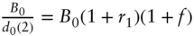 ;
; - Date 1:
 ;
; - Date 2:
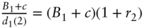
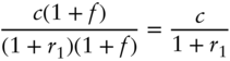
Therefore, the martingale property for the bond says that,
The term ![]() in the expectation on the right‐hand side of (A16.26) requires some attention, because
in the expectation on the right‐hand side of (A16.26) requires some attention, because ![]() is not known as of date 0. The date‐0 value of a payment of
is not known as of date 0. The date‐0 value of a payment of ![]() on date 2 is, however, by the definition of forward rates,
on date 2 is, however, by the definition of forward rates,
So, applying the martingale property under the numeraire to a payment of ![]() on date 2 requires that,
on date 2 requires that,
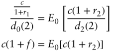
With this result, the discussion returns to the martingale property of the bond in (A16.26). Substituting (A16.28) into (A16.26),
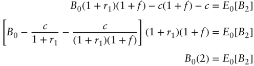
The left‐hand side of the second line of (A16.29) is the date 0 forward price of the bond for delivery on date 2. The third line, then, simply denotes this forward price by ![]() . Hence, taking the zero coupon bond of maturity
. Hence, taking the zero coupon bond of maturity ![]() as a numeraire, the forward price of a bond for delivery on date
as a numeraire, the forward price of a bond for delivery on date ![]() is a martingale.
is a martingale.
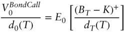
Turning now to the price of an option on the bond, consider a call with payoff ![]() . Applying the martingale property to the option price and assuming that the forward bond price is lognormal with volatility parameter
. Applying the martingale property to the option price and assuming that the forward bond price is lognormal with volatility parameter ![]() , the call option is priced as,
, the call option is priced as,
An analogous argument for a put shows that,
A16.3.2 Euribor Futures Options
The terminal payoff of a Euribor futures call option with strike ![]() and expiration time
and expiration time ![]() is, per unit notional,
is, per unit notional,
Given the daily settlement feature of Euribor futures options, the numeraire of choice is the money market account, the value of one unit of currency invested and then rolled every period, at the prevailing short‐term rate. Denoting the money market account by ![]() and the short‐term rate from time
and the short‐term rate from time ![]() to
to ![]() by
by ![]() ,
,
The first point to make about the money market account is that it is the numeraire of the risk‐neutral short‐term rate process used in the term structure models presented earlier in the book. To see this, apply the martingale property with the numeraire to an arbitrary gains process ![]() at time
at time ![]() ,
,
But the second line of (A16.37) is just the condition that the value of a claim today equals its expected discounted value.
The second point to make about the money markets as numeraire is that futures prices are martingales under this numeraire. This is proved in Section A16.5.
Turning now to Euribor futures options, because they are subject to daily settlement and are futures contracts, their prices are also martingales with the money market account as numeraire. Furthermore, if ![]() is the underlying futures price at time
is the underlying futures price at time ![]() , then at the expiration of a put option on the futures price (call on rates) at time
, then at the expiration of a put option on the futures price (call on rates) at time ![]() , the option is worth
, the option is worth ![]() . Putting together the martingale property of the futures, (A16.38), the martingale property of futures options, (A16.39), and the final settlement price of the futures options, (A16.40), results in the price of the Euribor futures put option at time
. Putting together the martingale property of the futures, (A16.38), the martingale property of futures options, (A16.39), and the final settlement price of the futures options, (A16.40), results in the price of the Euribor futures put option at time ![]() , denoted
, denoted ![]() ,
,
Assuming now that ![]() is normally distributed, applying Section A16.4 to Equations (A16.38) and (A16.40) shows that,
is normally distributed, applying Section A16.4 to Equations (A16.38) and (A16.40) shows that,
Similarly, for the Euribor futures call option (put on rates),
A16.3.3 Bond Futures Options
As shown in Section A16.5, futures prices are a martingale in the risk‐neutral measure, that is, when the numeraire is the money market account, ![]() . Hence, with
. Hence, with ![]() the underlying bond futures price at time
the underlying bond futures price at time ![]() ,
,
By the martingale property, the price of a put option on the futures is,
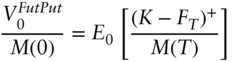
Then, by the definition of the money market account,

To continue, make the assumption – defended in the text – that the discount factor is uncorrelated with the futures price. Then, Equation (A16.45) becomes,
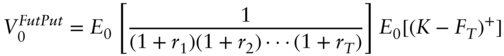
where (A16.47) follows from the risk‐neutral pricing of a zero coupon bond.
Finally, applying Section A16.5 to (A16.43), (A16.47) with the assumption that the bond futures price has a lognormal distribution,
For calls, the analogous result is,
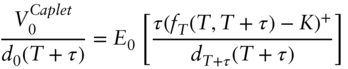
A16.3.4 Caplets
Caplets that mature at time ![]() are written on a forward rate from time
are written on a forward rate from time ![]() to
to ![]() , whose value, at time
, whose value, at time ![]() , is denoted by
, is denoted by ![]() . It is first shown that taking a
. It is first shown that taking a ![]() ‐year zero coupon bond as the numeraire makes this forward rate a martingale. Let
‐year zero coupon bond as the numeraire makes this forward rate a martingale. Let ![]() be the time‐
be the time‐![]() price of a zero coupon bond maturing at time
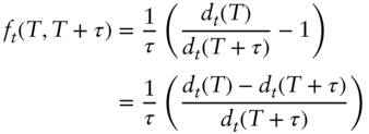
price of a zero coupon bond maturing at time ![]() . By the definition of a forward rate of term
. By the definition of a forward rate of term ![]() ,
,
Next, consider a portfolio that is long a ![]() ‐year zero and short a
‐year zero and short a ![]() ‐year zero. Taking the
‐year zero. Taking the ![]() ‐year zero as the numeraire, the normalized gains process of this portfolio is a martingale. Mathematically,
‐year zero as the numeraire, the normalized gains process of this portfolio is a martingale. Mathematically,
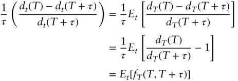
where the last line of (A16.51) just uses the definition of the forward rate. Combining (A16.50) and (A16.51) shows that the forward rate is a martingale under the chosen numeraire,
Turning to the valuation of the caplet, its normalized gains process is a martingale as well. Hence, taking expectations of its normalized gain as of ![]() ,
,
Finally, assuming that the forward rate ![]() is normal with variance
is normal with variance ![]() , and knowing from (A16.52) with
, and knowing from (A16.52) with ![]() that its mean is
that its mean is ![]() , the results of Section A16.4 apply and,
, the results of Section A16.4 apply and,
A16.3.5 Swaptions
The underlying of a ![]() ‐year into
‐year into ![]() ‐year swaption is the forward par swap rate from
‐year swaption is the forward par swap rate from ![]() to
to ![]() , which, at time
, which, at time ![]() , is denoted by
, is denoted by ![]() . It is first shown that taking an annuity from
. It is first shown that taking an annuity from ![]() to
to ![]() as the numeraire makes this forward par swap rate a martingale. Denote the price of this annuity by
as the numeraire makes this forward par swap rate a martingale. Denote the price of this annuity by ![]() .
.
Consider receiving the fixed‐rate ![]() on a swap from
on a swap from ![]() to
to ![]() . Its value at time
. Its value at time ![]() is,
is,
Applying the martingale property with this annuity as numeraire,

Hence, as claimed, the forward par swap rate is a martingale under this numeraire.
To price a receiver swaption, note that the payoff is ![]() ×
× ![]() . Therefore, its value can be calculated as the expectation of its normalized payoff using the same numeraire,
. Therefore, its value can be calculated as the expectation of its normalized payoff using the same numeraire,
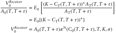
The last line of (A16.58) follows from (A16.57), the assumption that the forward par swap rate is normal with variance ![]() , and the appropriate result from Section A16.4.
, and the appropriate result from Section A16.4.
Similarly, a payer option under the assumption of normality has the value,
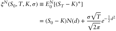
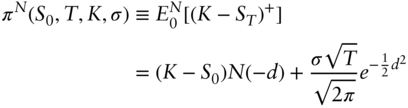
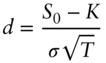
A16.4 EXPECTATIONS FOR BLACK‐SCHOLES‐MERTON STYLE OPTION PRICING
As the results in this section are part of the option pricing literature, they are presented here for easy reference but without proof. Let ![]() and
and ![]() denote the expectations operators under the normal and lognormal distributions, respectively, and let
denote the expectations operators under the normal and lognormal distributions, respectively, and let ![]() denote the standard normal cumulative distribution.
denote the standard normal cumulative distribution.
If ![]() is normally distributed with means
is normally distributed with means ![]() and variance
and variance ![]() , then,
, then,
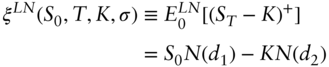
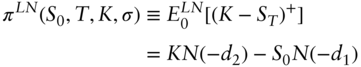
If ![]() is lognormally distributed with mean
is lognormally distributed with mean ![]() and variance
and variance ![]() , then,
, then,
A16.5 FUTURES PRICES ARE MARTINGALES WITH THE MONEY MARKET ACCOUNT AS A NUMERAIRE
The initial value of a futures contract is zero; subsequent cash flows are from daily settlements; and at maturity, the futures price is determined by some final settlement rule. Consider a two‐period, three‐date framework for simplicity, and let the futures price on date ![]() be
be ![]() . Then, the normalized gains process is,
. Then, the normalized gains process is,
- Date 0:
 ;
; - Date 1:
 ;
; - Date 2:
Since the value of a futures contact on date 0 is zero, the martingale property implies that the expectation of the normalized gains at any future date is zero. In particular, for date 1,

But since ![]() is known as of date 0, it follows from (A16.67) that,
is known as of date 0, it follows from (A16.67) that,
As of date 2, the martingale property says that
Using the law of iterated expectations, and the fact that ![]() is known as of date 0,
is known as of date 0,
But, since ![]() is known as of date 1, (A16.70) implies that,
is known as of date 1, (A16.70) implies that,
Finally then, combine (A16.68) and (A16.71) to see that,
Together with (A16.68), (A16.72) shows that the futures price is a martingale under the money‐market account or risk‐neutral measure, as desired.