APPENDIX TO CHAPTER 14
Corporate Debt and Credit Default Swaps
A14.1 CUMULATIVE DEFAULT AND SURVIVAL RATES
Proposition: If the hazard rate is constant at ![]() , then the cumulative survival probability to time
, then the cumulative survival probability to time ![]() ,
, ![]() , is
, is ![]() , and the cumulative default probability,
, and the cumulative default probability, ![]() , is
, is ![]() .
.
Proof: The probability of no default to time ![]() ,
, ![]() , is the probability that there is no default to time
, is the probability that there is no default to time ![]() and no default from then to time
and no default from then to time ![]() . Mathematically,
. Mathematically,
Taking the limit of the right‐hand side of (A14.2) as ![]() approaches zero is the derivative of
approaches zero is the derivative of ![]() , denoted
, denoted ![]() . Therefore,
. Therefore,
where Equation (A14.4) is the solution to Equation (A14.3). The cumulative default probability is just one minus the cumulative survival probability, which gives ![]() .
.
A14.2 UPFRONT AMOUNTS
Continue with the notation of the previous section, and add the following:
 : CDS spread
 : CDS coupon
 : maturity of the CDS, in years
 : number of CDS premium payments per year
 : time of CDS premium payment
  ,
,  , with
 : discount factor at time
  , at risk‐free or benchmark rates
 : recovery rate
 : upfront amount
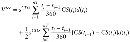
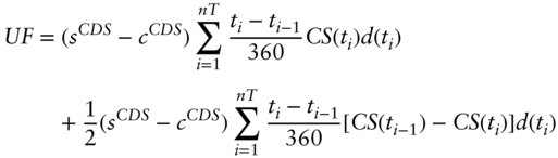
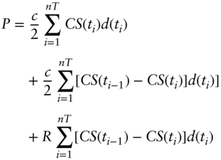
Then, following the logic described in the text, with the detail that premium payments follow the actual/360 day‐count convention, the expected discounted value of the fee leg, ![]() , is,
, is,
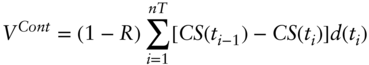
The value of the contingent leg, ![]() , again following the logic described in the text, is,
, again following the logic described in the text, is,
A CDS with a premium of ![]() is fair if the hazard rate is such that the values of the fee and contingent legs, as given in Equations (A14.5) and (A14.6), are equal.
is fair if the hazard rate is such that the values of the fee and contingent legs, as given in Equations (A14.5) and (A14.6), are equal.
The upfront amount, following the logic of the text, equals the expected discount value of paying the CDS coupon as a premium payment rather than the CDS spread. Essentially, the upfront amount is computed like the fee leg, with ![]() or
or ![]() replacing
replacing ![]() . Hence,
. Hence,
A14.3 AN APPROXIMATION FOR CDS SPREADS
For the purposes of this section, assume that premium payments of the CDS are all ![]() years apart, that is,
years apart, that is, ![]() for all
for all ![]() . Substituting that relationship into Equations (A14.5) and (A14.6) and setting the two equations equal, gives the following,
. Substituting that relationship into Equations (A14.5) and (A14.6) and setting the two equations equal, gives the following,
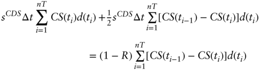
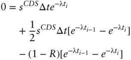
Substituting in from Equation (A14.4), each term of (A14.8) can be simplified as follows,
Furthermore, because ![]() for all
for all ![]() , it is easy to show that, if Equation (A14.9) holds for
, it is easy to show that, if Equation (A14.9) holds for ![]() , then it also holds for
, then it also holds for ![]() . Hence, in this special case,
. Hence, in this special case, ![]() can be solved from any one date. Proceeding then from Equation (A14.9), multiply through by
can be solved from any one date. Proceeding then from Equation (A14.9), multiply through by ![]() and simplify to see that,
and simplify to see that,
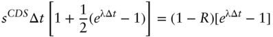
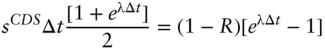
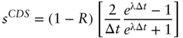
Finally, take the limit as ![]() approaches zero of the terms in the hard bracket on the right‐hand side of (A14.12) to obtain,
approaches zero of the terms in the hard bracket on the right‐hand side of (A14.12) to obtain,
A14.4 CDS‐EQUIVALENT BOND SPREADS
Following the logic of the text and this appendix, the expected discounted value of a bond's coupons can be computed along the lines of the fee leg of a CDS. Similarly, the expected discounted value of a bond's principal payment can be computed along the lines of the contingent leg, except that the payment from the bond upon default is ![]() times the principal amount, while the payment due to the buyer of protection upon default is
times the principal amount, while the payment due to the buyer of protection upon default is ![]() times the principal amount. Therefore, using Equations (A14.5) and (A14.6) – simplified here to assume that coupon payments are exactly one‐half years apart – the price of a bond,
times the principal amount. Therefore, using Equations (A14.5) and (A14.6) – simplified here to assume that coupon payments are exactly one‐half years apart – the price of a bond, ![]() , with a coupon rate,
, with a coupon rate, ![]() , given a hazard rate, is given by,
, given a hazard rate, is given by,
To solve for the CDS‐equivalent bond spread, find the hazard rate that solves Equation (A14.14). Then, using that hazard rate, find the ![]() that sets the fee leg in Equation (A14.5) equal to the contingent leg in Equation (A14.6).
that sets the fee leg in Equation (A14.5) equal to the contingent leg in Equation (A14.6).
A14.5 BOND SPREAD WITH MARKET RECOVERY
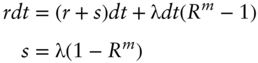
From the definition of bond spread, if the bond does not default (and rates do not change), then the return on the bond equals the risk‐free or benchmark rate, ![]() , plus the spread. If the bond defaults and recovers
, plus the spread. If the bond defaults and recovers ![]() of its market price, then the return over the moment of default is
of its market price, then the return over the moment of default is ![]() or
or ![]() . Therefore, over a short time interval
. Therefore, over a short time interval ![]() years, over which the probability of no default and default are
years, over which the probability of no default and default are ![]() and
and ![]() , respectively, the expected return on the bond is,
, respectively, the expected return on the bond is,
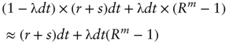
where the approximation follows from ignoring the very small terms, that is, those that are multiplied by ![]() .
.
Assuming that investors are risk neutral or that the hazard rate is a risk‐neutral pricing rate, investors are indifferent between buying a corporate bond and buying a bond without default risk if the expected return of the former, given in Equation (A14.15), is equal to the risk‐free rate. Mathematically, then,