
Chapter 11
Making Queries Work Together
In This Chapter
![]() Reusing query steps
Reusing query steps
![]() Consolidating data with the Append feature
Consolidating data with the Append feature
![]() Understanding join types
Understanding join types
![]() Using the Merge feature
Using the Merge feature
Data is frequently analyzed in layers, with each layer of analysis using or building on the previous layer. You may not know it, but you already build layers all the time. For instance, when you build a pivot table using the results of a Power Query output, you’re layering your analysis. When you build a query based on a table created by a SQL Server view, you’re also creating a layered analysis.
Sure, you would probably love to be able to analyze a single data source and call it a day. But that’s not how data analysis works. You often find the need to build queries on top of other queries to get the results you’re looking for. That’s what this chapter is all about. In this chapter, I help you examine a few ways you can advance your data analysis by making your queries work together.
Reusing Query Steps
Data analysts commonly rely on the same main data tables for all kinds of analysis. Even the simple table shown in Figure 11-1 can be used to create different views: sales by employee, sales by business segment, or sales by region, for example.
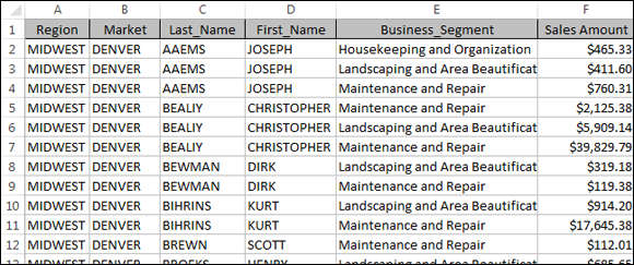
Figure 11-1: This data can be used as the source for various levels of aggregated analysis.
Of course, you can build separate queries, each performing different grouping and aggregation steps, but that would mean repeating all the data clean-up steps you needed before performing any kind of analysis.
To get a better understanding of how query steps can help save time, take a moment to follow these steps:
- Open the Sales By Employee.xlsx workbook, found in the sample files for this book.
Place the cursor anywhere inside the table, and then choose Data ⇒ From Table.
Power Query opens the Query Editor.
- While in the Query Editor, click the Filter drop-down list for the Market field and filter out the Canada market. (Remove the check mark next to Canada.)
Select the Last_Name and First_Name fields, and then choose Transform ⇒ Merge Columns.
The Merge Columns dialog box appears.
- Create a new Employee field, joining Last_Name and First_Name and separating them by a comma, as shown in Figure 11-2.
Click the Group By command on the Transformation tab.
The Group By dialog box opens, as shown in Figure 11-3.
The goal is to Group By the Employee field to get the Sum of Sales Amount, as shown in Figure 11-3. Name the new aggregated column Revenue.
At this point, you’ve successfully created a view that shows total revenue by employee. As you can see in Figure 11-4, the query steps include all the preparation work you did before grouping.
What happens if you want to create another analysis using the same data? For instance, what if you want another view that shows Employee sales by business segment?
You could always start from Step 1 and import another copy of the source data, but you’d have to repeat the preparation steps (the steps for Filtered Rows and Merged Columns, in this case).
A better way is to reuse the steps you’ve already created by extracting them into a new query. The idea is to first decide what steps you want to reuse and then right-click the step immediately below it. In this scenario (refer to Figure 11-4), you keep all query steps until Grouped Rows.
Right-click the Grouped Rows step and select Extract Previous.
The Extract Steps dialog box opens.
- Name the new query SalesByBusiness, as shown in Figure 11-5. Click the OK button confirm.
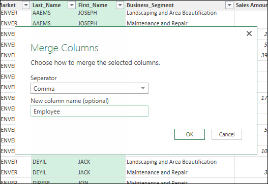
Figure 11-2: Merge the Last_Name and First_Name columns to create a new Employee field.
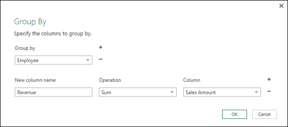
Figure 11-3: Group the Employee field and Sum Sales Amount to create a new Revenue column.
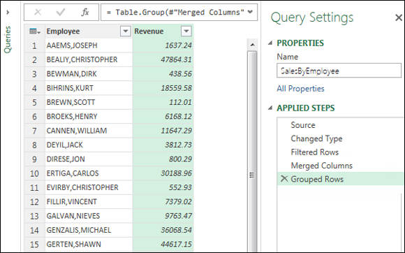
Figure 11-4: All the query steps before Grouped Rows are needed in order to prepare the data for grouping.

Figure 11-5: Naming the new query SalesByBusiness.
After you click OK, Power Query does two things:
- Moves all extracted steps to the newly created query
- Ties the original query to the new query
That is to say, both queries are sharing the extracted steps. You can see the new SalesByBusiness query in the pane on the left, as shown in Figure 11-6.
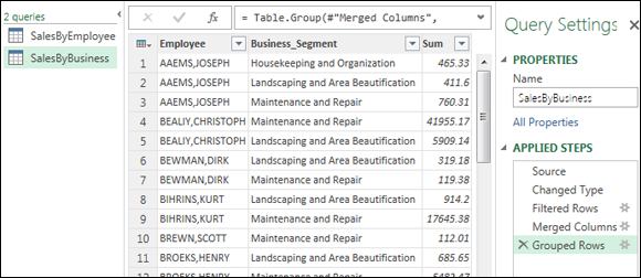
Figure 11-6: The two queries are now sharing the extracted steps.
You now can click on the SalesByBusiness query and start applying any needed transformations. In Figure 11-6, a Group By step has been added to create a view of sales by employee and by business segment.
This concept of extracting steps can be a bit confusing. The bottom line is that instead of starting from square one with a brand-new query, you’re telling Power Query you want to create a new query that uses the steps you’ve already created.
 When two or more queries share extracted steps, the query that contains the extracted steps serves as the data source for the other queries. Because of this link, the query that contains the extracted steps cannot be deleted. You have to first delete all dependent queries before deleting the query that holds the extracted steps.
Understanding the Append Feature
Power Query’s Append feature allows you to add the rows generated from one query to the results of another query. In other words, you copy records from one query and add them to the end of another.
The Append feature comes in handy when you need to consolidate multiple identical tables into one table. For example, if you have tables from the North, South, Midwest, and West regions, you can consolidate the data from each region into one table using the Append feature.
To help you better understand the Append feature, I’ll walk you through an exercise that consolidates data from four different regions into one table. In this walk-through, I use the region data found on four different tabs in the Appending_Data.xlsx sample file, shown in Figure 11-7.
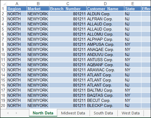
Figure 11-7: The data found on each region tab needs to be consolidated into one table.
 You can find the Appending_Data.xlsx workbook in the sample files for this book.
Creating the needed base queries
The Append feature works on only existing queries. That is to say, no matter what kind of data sources you have, you need to import them into Power Query before you can append them together. In this case, it means importing all the region tables into queries.
Follow these steps to import the needed base queries:
Go to the North Data worksheet, place the cursor anywhere inside the table, and then choose Data ⇒ From Table.
The Query Editor activates, showing you the contents of the table you just imported.
To finalize the creation of the query, you need to close and load the query. Now, because you’re creating this query simply for the purpose of appending it to other queries, you don’t need to close and load to the workbook. You can choose instead to close and load the data as connection-only.
- On the Home tab of the Query Editor, click the drop-down arrow under the Close & Load command and select Close & Load To.
- In the Load To dialog box, choose the option Only Create Connection, and then click the Load button.
- Repeat Steps 1 through 3 for the other worksheets in the workbook.
After you’ve created queries for each region, open the Workbook Queries pane (choose Data ⇒ Show Queries) to see all queries. As you can see in Figure 11-8, each query is a connection-only query.
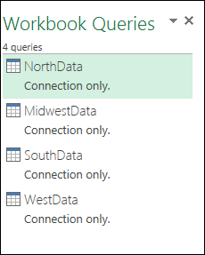
Figure 11-8: Create a connection-only query for each region.
Now that your data is in queries, you can start appending.
Appending the data
In a perfect world, this section is where you would read about the nifty button that appends all your queries at one time. Unfortunately, Power Query doesn’t have a nifty button that lets you append many tables all in one shot. You can append only one table at a time.
To append data, follow these steps:
- In the Workbook Queries pane, right-click on the NorthData query and select Edit to open the Query Editor.
On the Home tab of the Query Editor, click the Append Queries command.
The Append dialog box opens.
- The drop-down menu contains a list of all queries in the current workbook, as shown in Figure 11-9. The idea is to select the query you want to append to the query you’re editing. Select one of the region queries, and then click the OK button.
- Repeat Steps 2 and 3 until you’ve appended the SouthData, MidwestData, and WestData queries.
After all queries have been appended, click the Close & Load command to save the data and exit the Query Editor.
At this point, the NorthData query contains the data for all regions. To see the full consolidated table, you need to change the load destination of the NorthData query to the workbook instead of the connection only.
In the Workbook Queries pane, right-click the NorthData query and select Load To.
The Load To dialog box opens.
- Select the option for Table, and then click OK.
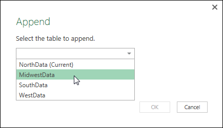
Figure 11-9: Select the query that you want appended to the query you’re editing.
Figure 11-10 illustrates the final output. You’ve successfully created a consolidated table of region data.
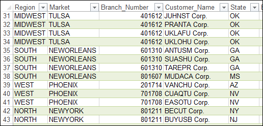
Figure 11-10: The final consolidated table of all region data.
 Note in Figure 11-9 the option for NorthData (Current). You see the term (Current) next to the NorthData query because you’re editing that query. Be careful not to select any query with (Current) next to it. Otherwise, you’ll append the query to itself, effectively duplicating all records within the query. Unless you have some strange requirement where creating exact copies of records is beneficial, avoid appending the current query to itself.
As you append each query, you may be tempted to scroll down to the bottom of the data to see the newly added records. Unfortunately, the data preview in the Query Editor shows only a truncated sample set of records. Even if you scroll to the bottom of the preview, you’re unlikely to see the appended data.
Understanding the Merge Feature
In your data adventures, you often find the need to build queries that join the data between two tables. For example, you may want to join an employee table to a transaction table to create a view that contains both transaction details and information on the employees who logged those transactions.
In this section, I describe how you can leverage the Merge feature in Power Query to join data from multiple queries.
Understanding Power Query joins
Similar to VLOOKUP in Excel, the Merge feature joins the records from one query to the records in another by matching on a unique identifier. An example of a unique identifier is Customer ID or Invoice Number.
You can join two datasets in one of several ways. The kind of join you apply is important because it determines which records are returned from each dataset.
Power Query supports six kinds of joins, as described in the following list and shown in Figure 11-11:
- Left Outer: Tells Power Query to return all records from the first query, regardless of matching, and only those records from the second query that have matching values in the joined field.
- Right Outer: Tells Power Query to return all records from the second query, regardless of matching, and only those records from the first query that have matching values in the joined field.
- Full Outer: Tells Power Query to return all records from both queries, regardless of matching.
- Inner: Tells Power Query to return only those records from both queries that have matching values.
- Left Anti: Tells Power Query to return only those records from the first query that don’t match any of the records from the second query.
- Right Anti: Tells Power Query to return only those records from the first query that don’t match any of the records from the second query.

Figure 11-11: The kinds of joins supported by Power Query.
Merging queries
To better understand the Merge feature, I’ll walk you through an exercise that merges interview questions and answers. In this walk-through, I use the predefined queries found in the Merging_Data.xlsx sample file available online at www.dummies.com/go/excelpowerpivotpowerqueryfd.
As you can see in Figure 11-12, two existing queries are in the Workbook Queries pane: Questions and Answers. These queries represent the questions and answers from the interview. The goal is to merge these two queries to create a new table showing questions and answers side-by-side.
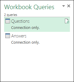
Figure 11-12: You need to merge the Questions and Answers queries into one table.
The Merge feature can be used only with existing queries. That is to say, no matter what kind of data sources you have, you need to import them into Power Query before you can use them in a merge.
Follow these steps to perform the merge:
Choose Data ⇒ New Query ⇒ Combine Queries ⇒ Merge (see Figure 11-13).
This step opens the Merge dialog box.
In this dialog box, you use the drop-down boxes to select the queries you want to merge and then choose the columns that defined the unique identifier for each record. In this case, the InterviewID and QuestionID/AnswerID fields make up the unique identifier for each record.
- Select the Questions query in the top drop-down box.
- Hold down the Ctrl key on the keyboard, and then click InterviewID and QuestionID — in that order.
- Select the Answers query in the lower drop-down box.
- Hold down the Ctrl key on the keyboard, and then click InterviewID and AnswerID — in that order.
- Use the Join Kind drop-down box to select the kind of join you want Power Query to use. In this case, the default, Left Outer, works.
Click the OK button to finalize and open the Query Editor.
In Figure 11-14, note the small numbers 1 and 2 in the InterviewID and QuestionID fields. These small numbers are assigned based on the order in which you selected them (refer to Steps 3 and 5).
The order in which you selected the unique identifiers in each query matters. The two columns tagged with the small number 1 will be joined regardless of column labels. The two columns tagged with the small number 2 will also be joined.
At the bottom of the Merge dialog box, Power Query shows you how many records from the lower query match the top query, based on the unique identifiers you selected. In this case, about 17,600 answer records match the 26,910 question records.
You don’t need a 100 percent match for the merge to be valid. There might be a good reason that the records in the two queries don’t all match up. In this case, not all questions were answered in all interviews, so the Answers query has fewer records.With the new merged query open in the Query Editor, click the Expand icon in the NewColumn field and choose the fields you want included in the final output (as shown in Figure 11-15). In this case, just choose the Answer field.
At this point, you can apply more transformations, if needed.
When you’re happy with the way things look, click the Close & Load command to output the results to the workbook.
Figure 11-16 shows the final merged query.
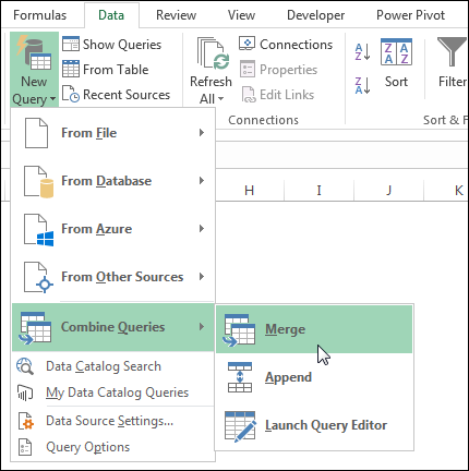
Figure 11-13: Activating the Merge dialog box.
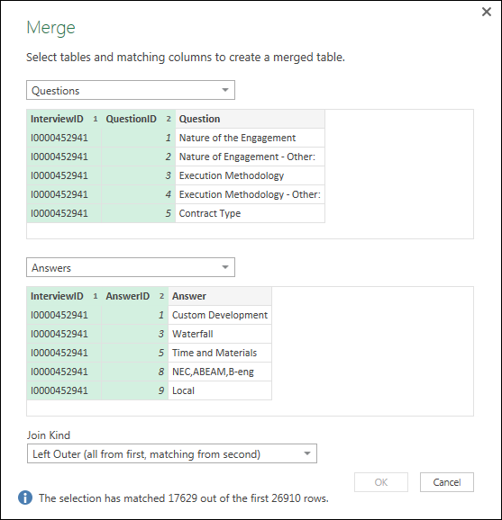
Figure 11-14: The Merge dialog box.
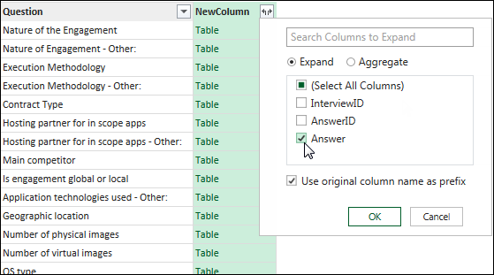
Figure 11-15: Expand the NewColumn field and choose the merged fields you want to output.
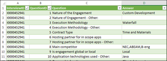
Figure 11-16: The final table with merged questions and answers.
If you need to adjust or correct a merged query, right-click the query in the Workbook Queries pane and select Edit. In the Query Editor, click the Gear icon next to the Source query step, as shown in Figure 11-17. This action opens the Merge dialog box, where the necessary changes can be applied.
Figure 11-17: Click the Gear icon next to the Source query step to reopen the Merge dialog box.