
Chapter 10
Transforming Your Way to Better Data
In This Chapter
![]() Performing common transformations
Performing common transformations
![]() Creating your own custom columns
Creating your own custom columns
![]() Understanding data types
Understanding data types
![]() Understanding Power Query formulas
Understanding Power Query formulas
![]() Applying conditional logic
Applying conditional logic
![]() Grouping and Aggregating Data
Grouping and Aggregating Data
Wouldn’t it be great if all the data sources you work with were clean and ready to use? Unfortunately, that’s not the case — you often receive data that is unpolished, or raw. That is to say, the data may have duplicates or blank fields or inconsistent text, for example.
Data transformation generally entails certain actions that are meant to “clean” your data — actions such as establishing a table structure, removing duplicates, cleaning text, removing blanks, and even adding your own calculations.
In this chapter, I introduce you to some of the tools and techniques in Power Query that make it easy for you to clean and massage your data.
 You can follow along with the examples in this chapter by downloading the LeadList.txt sample file from
 www.dummies.com/go/excelpowerpivotpowerqueryfd. After you download it, you can import the sample file into Power Query: Select Data ⇒ New Query ⇒ From File ⇒ From Text and then point to LeadList.txt.
Completing Common Transformation Tasks
Many of the unpolished datasets that come to you will require other types of transformation actions. This section covers some of the more common transformation tasks you will have to perform, such as removing duplicates, finding and replacing text, filling empty cells, and splitting or joining text values.
Removing duplicate records
Duplicate records are absolute analysis killers. The effect that duplicate records have on your analysis can be far-reaching, corrupting almost every metric, summary, and analytical assessment you produce. It is for this reason that finding and removing duplicate records should be your first priority when you receive a new dataset.
Before you begin examining the dataset to find and remove duplicate records, consider how you define a duplicate record. Look at the table shown in Figure 10-1, where you see 11 records. Of the 11 records, how many are duplicates?

Figure 10-1: Does this table have duplicate records? It depends on how you define them.
If you were to define a duplicate record in Figure 10-1 as a duplication of only the SicCode, you would find 10 duplicate records. That is, of the 11 records shown, 1 record has a unique SicCode, and the other 10 are duplications. Now, if you were to expand your definition of a duplicate record to a duplication of both SicCode and PostalCode, you would find only two duplicates: the duplication of postal codes 77032 and 77040. Finally, if you were to define a duplicate record as a duplication of the unique value of SicCode, PostalCode, and CompanyNumber, you would find no duplicates.
This example shows that having two records with the same value in a column doesn’t necessarily mean that you have a duplicate record. It’s up to you to determine which field or combination of fields best defines a unique record in the dataset.
After you have a clear idea of which field or fields best make up a unique record in the table, you can remove duplicates easily by using the Remove Duplicates command.
Figure 10-2 illustrates the removal of duplicate rows based on three columns. Note the importance of selecting the columns that define a duplicate. In this case, the combination of Address, CompanyNumber, and CompanyName defines a duplicate record. You select these columns before clicking the Remove Duplicates command on the Home tab of the Power Query ribbon.

Figure 10-2: Removing duplicate records.
 The Remove Duplicates command essentially looks for distinct values in the columns you selected and then removes all records necessary to end up with a unique list of values. If you select only one column before giving the Remove Duplicates command, Power Query uses only one column you selected to determine the unique list of values, which undoubtedly removes too many records — records that aren’t truly duplicates. For this reason, be sure to select all columns that define a duplicate.
If you make a mistake and remove duplicates based on the wrong set of columns, don’t worry: You can always use the Query Settings pane to delete that step. Right-click on the Removed Duplicates step and select Delete (see Figure 10-3). Alternatively, you can click the X next to the Remove Duplicates step.

Figure 10-3: Undo the removal of records by deleting the Removed Duplicates step.
 If you don’t see the Query Settings pane, select View ⇒ Query Settings to activate the Query Settings pane.
Filling in blank fields
There are two kinds of blank values: null and empty string. A null is essentially a numerical value of nothing, whereas an empty string is equivalent to entering two quotation marks (“”) in a cell.
Blank fields aren’t necessarily a bad thing, but having an excessive number of blanks in your data can lead to unexpected problems when analyzing it.
Your job is to decide whether to leave the blanks in the dataset or fill them with actual values. Consider the following best practices:
- Use blanks sparingly: Working with a dataset is a much less daunting task when you don't have to test continually for blank values.
- Use alternatives whenever possible: Represent missing values with some logical missing-value code whenever possible.
- Never use null values in number fields: Use zero instead of null in a currency or a number field that will be used in calculations.
Replacing null values
Power Query shows the word null for any null value in your data. Replacing the null values is as simple as selecting the column or columns you want to fix and then selecting the Replace Values command, as shown in Figure 10-4.

Figure 10-4: Activating the Replace Values dialog box.
The Replace Values dialog box, shown in Figure 10-5, opens. After you enter the word null as the value to find, you can then enter the value you want to use instead. In this case, enter 0 as the Replace With value.
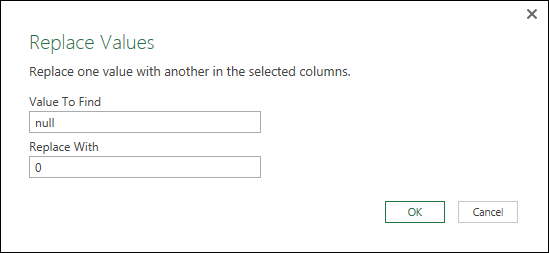
Figure 10-5: Replacing null with 0.
Filling in empty strings
To follow best practices, represent missing values in a field with some logical value code whenever possible. For example, in Figure 10-6, I want to tag with the word Undefined any record with a missing title in the ContactTitle field.

Figure 10-6: Replacing empty strings with the word Undefined.
You can do so by clicking on ContactTitle, selecting the Replace Values command, and then entering the word Undefined in the Replace Values dialog box. As you can see in Figure 10-6, because you’re replacing an empty string, there’s no need to enter anything in the Value to Find input box.
If you need to adjust or correct the step where you replace values, you can reopen the Replace Values dialog box by clicking the Gear icon next to the name for that step. This is true for any action that requires a dialog box to complete. Clicking on the Gear icon next to any step name opens the appropriate dialog box for that step.
Concatenating columns
You can easily concatenate (join) the values in two or more columns. In Power Query, you do this by using the Merge Columns command. The Merge Columns command concatenates the values in two or more fields and outputs the newly merged values into a new column.
First choose the columns you want to concatenate, and then select the Transform tab and then the Merge Columns command, as shown in Figure 10-7.

Figure 10-7: Merging the Type and Code fields.
The Merge Columns dialog box opens, as shown in Figure 10-8. You have the option of choosing from a list of the most commonly used delimiters (comma, space, tab, etc.). You can also select the Custom option to enter your own delimiter. In Figure 10-8, a hyphen (-) is used.
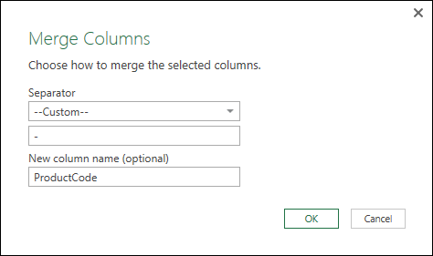
Figure 10-8: The Merge Columns dialog box.
As you can see, you can also name the new column that will be created.
The reward for your efforts is a new field containing the concatenated values from the original column (see Figure 10-9). The resulting column will be named Merged. You can rename the column by right-clicking it and selecting the Rename option.

Figure 10-9: The original columns are removed and replaced with a new, merged column.
This feature is nifty, but notice that Power Query removes the original Type and Code columns. In some instances, you’ll definitely want to concatenate values but retain the source columns. In those instances, the answer is to create your own, custom column. Later in this chapter, I describe how to use custom columns to solve this and other transformation problems.
Changing case
Making sure that the text in your data has the correct capitalization may sound trivial, but it’s important. Imagine that you receive a customer table that has an address field where all addresses are lowercase. How will that look on labels, form letters, or invoices? Fortunately, Power Query has a few built-in functions that make changing the case of your text a snap.
For example, the ContactName field (see Figure 10-10) contains names that are formatted in all uppercase letters. To change these names to the more appropriate proper case, you can use the Format command found on the Transform tab. The Format command has options for lowercase, uppercase and proper case (capitalize each word).

Figure 10-10: Reformatting the ContactName field to proper case.
 Selecting the Capitalize Each Word option reformats all values in the selected column to proper case.
Finding and replacing specific text
Imagine that you work in a company named BLVD, Inc. One day, the president of your company informs you that the abbreviation blvd on all addresses is now deemed an infringement of your company’s trademarked name and must be changed to Boulevard as soon as possible. How would you go about meeting this new requirement?
The Replace Values function is ideal in a situation like this. Select the Address field, and then click the Replace Values command on the Home tab.
In the Replace Values dialog box (shown in Figure 10-11), simply fill the Value to Find input box with the value you want to find, and then fill the Replace With input box with the value you want to use as a replacement.

Figure 10-11: Replacing text values.
Note that clicking on Advanced Options reveals two optional settings, which are described in this list:
- Match entire cell contents: Selecting this option tells Power Query to replace values that contain only the text entered into the Value to Find field. This option comes in handy when you want to replace zeros (0) with n/a but not affect any zeros that are part of a number — only those that are alone in a cell.
- Replace Using Special Characters: Selecting this option allows you to use special invisible characters such as line feed, carriage return, or tab as replacement text. This option is useful when you want to force an indent or reposition the text so that it shows up on two lines.
Trimming and cleaning text
When you receive a dataset from a mainframe system, a data warehouse, or even a text file, it isn’t uncommon to have field values that contain leading and trailing spaces. These spaces can cause some abnormal results, especially when you’re appending values with leading and trailing spaces to other values that are clean. To demonstrate this concept, look at the dataset in Figure 10-12.

Figure 10-12: Leading spaces can cause issues in analysis.
This view is intended to be an aggregate view that displays the sum of the dollar potential for California, New York, and Texas. However, the leading spaces are forcing each state into two sets, preventing you from discerning the accurate totals.
You can easily remove leading and trailing spaces by using the Trim function in Power Query. Figure 10-13 demonstrates how you would update a field to remove the leading and trailing spaces by using the Trim command found on the Transformation tab.

Figure 10-13: The Trim command.
Again, the Trim command is applied to any column or columns you select. So, you can fix multiple columns at a time by simply selecting them before selecting the Trim command.
Figure 10-13 also shows the Clean command (beneath Trim). Whereas Trim removes leading and trailing spaces, the Clean command removes any invisible characters, such as carriage returns and other nonprintable characters that may slip in from external source systems. These characters are typically rendered in Excel as question marks or square boxes. But in Power Query, they show up as spaces.
If the source system that supplies your data has a nasty habit of including strange characters and leading spaces, you can apply the Trim and Clean functions to sanitize the dataset.
You may already know that the TRIM function in Excel removes the leading spaces, trailing spaces, and excess spaces within the given text. Power Query’s Trim function removes leading and trailing spaces, but doesn’t touch the excess spaces in the text. If excess spaces are a problem in your data, you can deal with them by using the Replace Values function to replace a given number of spaces with only one space.
Extracting the left, right, and middle values
In Excel, the RIGHT function, the LEFT function, and the MID function allow you to extract portions of a string starting from different positions:
- Left: Returns a specified number of characters, starting from the leftmost character of the string. The required arguments for the Left function are the text you’re evaluating and the number of characters you want returned. For example, Left(“70056-3504”, 5) would return five characters starting from the leftmost character (“70056”).
- Right: Returns a specified number of characters starting from the rightmost character of the string. The required arguments for the Right function are the text you’re evaluating and the number of characters you want returned. For example, Right(“Microsoft”, 4) would return four characters starting from the rightmost character (“soft”).
- Mid: Returns a specified number of characters starting from a specified character position. The required arguments for the Mid function are the text you’re evaluating, the starting position, and the number of characters you want returned. For example, Mid(“Lonely”, 2, 3) would return either three characters starting from the second character or character number 2 in the string (“one”).
Power Query has equivalent functions exposed through the Extract command, found on the Transformation tab (see Figure 10-14). The Extract command allows you to get specified characters from a value.

Figure 10-14: The Extract command allows you to pull out parts of the text found in a column.
The options under the Extract command are described in this list:
- Length: Transforms a given column into numbers that represent the number of characters in each row (similar to Excel’s LEN function).
- First Characters: Transforms a given column to show a specified number of characters from the beginning of text in each row (similar to Excel’s LEFT function).
- Last Characters: Transforms a given column to show a specified number of characters from the end of text in each row (similar to Excel’s RIGHT function).
- Range: Transforms a given column to show a specified number of characters starting from a specified character position (similar to Excel’s MID function).
Applying the Extract command to a column effectively replaces the original text with the results of the operation you choose to apply. That is to say, the original text isn’t visible in the table after you apply the Extract command. For this reason, you may want to first copy the column and perform the extraction on the duplicate column.
You can create a copy of a column by right-clicking on the column and selecting Duplicate Column. When the duplicate column is created, it’s the last (rightmost) column of the table.
Extracting first and last characters
To extract the first N characters of text, highlight the column, select Extract ⇒ First Characters, and then use the dialog box shown in Figure 10-15 to specify the number of characters you want to extract. In this case, the first three characters of the Phone field are extracted.

Figure 10-15: Extracting the first three characters of the Phone field.
To extract the last N characters of text, highlight the column, select Extract ⇒ Last Characters, and then use the dialog box to specify the number of characters you want extracted.
Extracting middle characters
To extract the middle N characters of text, highlight the column and select Extract ⇒ Range. The dialog box shown in Figure 10-16 opens.

Figure 10-16: Extracting the two middle characters of the SicCode.
The idea here is to tell Power Query to extract a specific number of characters starting from a certain position in the text. For example, the SicCode field is a 4-digit field. If you want to extract the two middle numbers of the SicCode, you would tell Power Query to start at the second character and extract two characters from there.
As you can see in Figure 10-16, the starting index is set to 2 (starting at the second character) and the number of characters is set to 2 (extract two characters from the starting index).
Splitting columns using character markers
Have you ever gotten a dataset where two or more distinct pieces of data were jammed into one field and separated by commas? For example, a field labeled Address may have a single text value that represents address, city, state, and postal code. In a proper dataset, this text would be split into four fields.
In Figure 10-17, you can see that the values in the ContactName field are strings that represent Last name, First name, and Middle initial. Imagine that you need to split this column string into three separate fields.

Figure 10-17: The Split Column command can easily split the ContactName Field into three separate columns.
Although this isn’t a straightforward undertaking in Excel, it can be done fairly easily with the Split Column command (found on the Transformation tab).
Selecting the Split Column command reveals two options; this list describes what you can do with them:
- By Delimiter: Split a column based on specific characters such as commas, semicolons, or spaces. This option is useful for parsing names or addresses or any field that contains multiple data points separated by delimiting characters.
- By Number of Characters: Split a column based on a specified number of characters — useful for parsing uniform text at a defined character position.
In the example (refer to Figure 10-17), the contact names are made up of last names, first names, and middle initials, all separated (delimited) by commas. So the By Delimiter option is the one I show you how to use.
You can highlight the ContactName field and select Split Column ⇒ By Delimiter to open the Split by Column Delimiter dialog box, shown in Figure 10-18.

Figure 10-18: Splitting the ContactName column at every occurrence of a comma.
This list describes the inputs:
- Select or Enter Delimiter: Use the drop-down menu to choose the delimiter that will define where the values should be split. If the delimiter isn’t listed as a choice on the drop-down list, you can select the Custom option and define your own.
- Split: Select how you want Power Query to use the specified delimiter. Power Query can split the column only on the first occurrence of the delimiter (the leftmost delimiter) — effectively creating two columns. Alternatively, you can tell Power Query to split the column only on the last occurrence of the delimiter (the rightmost delimiter) — again, creating two columns. The third option is to tell Power Query to split the column at each occurrence of the delimiter.
- Advanced Options: By default, selecting the option to split the column at each occurrence of the delimiter creates as many columns as there are delimiters. You can use the advanced options to override the default and limit the number of columns to create.
Figure 10-19 shows the new columns created after the ContactName column is split at each comma. As you can see, three new fields are created. You can rename a field by right-clicking the field name and selecting the Rename option.

Figure 10-19: The ContactName field has been split successfully into three columns.
Pivoting and unpivoting fields
You often encounter data sets like the one shown in Figure 10-20, where important headings (like Month) are spread across the top of the table, pulling double duty as column labels and actual data values. This matrix layout is easy to look at in a spreadsheet, but it causes problems when attempting to perform any kind of data analysis that requires aggregation or grouping, for example.

Figure 10-20: Matrix layouts are problematic for data analysis.
Power Pivot offers an easy way to unpivot and pivot columns, allowing you to quickly convert matrix-style tables to tabular datasets (and vice versa).
Unpivot Columns command
The Unpivot Columns command lets you select a set of columns and convert those columns into two columns: one column consisting of the old column labels and another containing the old column data.
For instance, in Figure 10-21, the month columns can be unpivoted by selecting the months and then clicking the Unpivot Columns command.

Figure 10-21: Unpivoting a matrix-style Month report.
The resulting table is shown in Figure 10-22. Note that the month labels are now entries in a new column named Attribute. The month values are now in a new column named Value. You can, of course rename these columns to Month and Revenue, for example.

Figure 10-22: All months are now in a tabular format.
Unpivot Other Columns command
As helpful as the Unpivot Columns command is, it has a flaw: You have to explicitly select the months that you want unpivoted. But what if the number of columns is ever growing? What if you unpivot January through June, but next month a new dataset will arrive with July and then August and then September? Because the Unpivot Columns command forces you to essentially hard-code the columns you want unpivoted, you have to redo the unpivot each and every month.
Fortunately, you can avoid this problem with the Unpivot Other Columns command. This nifty command allows you to unpivot by selecting the columns that you want to remain static and telling Power Query to unpivot all other columns.
For instance, Figure 10-23 demonstrates that rather than select the month columns, you can select the Market and Product_Description columns and then select Unpivot Other Columns from the Unpivot Columns drop-down menu.

Figure 10-23: Use Unpivot Other Columns when the number of matrix columns is variable.
Now, it doesn’t matter how many new month columns are added or removed each month. Your query always unpivots the correct columns.
Always use the Unpivot Other Columns option. Even if you don’t anticipate new matrix columns, it’s always a good bet to use the option that offers more flexibility for those unexpected changes in data.
Pivot Columns command
If you find that you need to transform your data from a tabular layout to a matrix-style layout, you can use the Pivot Columns command.
Simply select the columns that will make up the header labels and values for the new matrix columns, and then select the Pivot Column command, shown in Figure 10-24.

Figure 10-24: Pivoting the Month and Value columns.
Before finalizing the pivot operation, Power Query opens a dialog box (shown in Figure 10-25) to confirm the value column and the aggregation method. By default, Power Query uses the Sum operation to aggregate the data into the matrix format. You can override this default setting by selecting a different operation (count, average, or median, for example). You can even specify that you don’t want aggregation performed. Clicking the OK button finalizes the pivot operation.

Figure 10-25: Confirm the aggregation operation to finalize the pivot transformation.
Creating Custom Columns
When transforming your data, you sometimes have to add your own columns to extract key data points, create new dimensions, or even create your own calculations.
You start a new custom column by going to the Add Column tab and clicking the Add Custom Column command (see Figure 10-26). This opens the Add Custom Column dialog box.

Figure 10-26: Adding a custom column.
The Add Custom Column dialog box (shown in Figure 10-27) is your workbench for adding your own functionality to the query by using Power Query formulas. That’s right: When you add a new custom column, it doesn’t do anything until you provide a formula that gives it some utility.

Figure 10-27: The Add Custom Column dialog box.
As for the Add Custom Column dialog box, there’s not much to it. The inputs are described in this list:
- New column name: An input box where you enter a name for the column you’re creating.
- Available columns: A list box that contains the names of all columns in the query. Double-click any column name in this list box to automatically place it in the formula area.
- Custom column formula: The area where you type the formula.
As in Excel, a formula can be as simple as =1 or as complicated as an if statement that applies some conditional logic. Over the next few sections, I walk you through a few examples of creating custom columns to go beyond the functionality provided via the user interface.
But before diving into building Power Query formulas, you should understand how Power Query formulas differ from those in Excel. Here are some high-level differences to be aware of:
- No cell references. You can’t reach outside the Add Custom Column dialog box to select a range of cells. Power Query formulas work by referencing columns, not cells.
- Excel functions don’t work. The Excel functions you’re used to don’t work in Power Query. Power Query has many of the same kinds of functions as Excel, but it has its own formula language.
- Everything is case sensitive. In Excel, you can type in all lowercase or all uppercase letters and your formulas will work. Not so in Power Query. To Power Query, sum, Sum, and SUM are three different items, and only one of them is acceptable.
- Data types matter. Some fields are text fields, other fields are number fields, and still others are date fields. Excel does a good job of handling formulas that mix fields of differing data types. The Power Query formula language, which is extremely sensitive to data types, doesn’t have the built-in intelligence to gracefully handle data type mismatches. Data type issues are resolved with conversion functions, as covered later in this chapter.
- No tool tips or intelligence help. Excel is quick to throw up a tool tip or a menu of options when you start entering a new formula. Power Query has none of that. As of this writing, Power Query offers only a Learn About Power Query Formulas link to a Microsoft site dedicated to Power Query.
Don’t panic. Power Query formulas are not as gloomy as they sound. Let’s start with a simple custom column.
Concatenating with a custom column
Earlier in this chapter, I tell you how to concatenate values from two or more columns by using the Merge Columns command. Although this command is easy to use, it results in the original source columns being removed. You will likely want to concatenate values but still retain the source columns.
In these instances, you can create your own custom column. Follow these steps to create a new column that merges the Type and Code columns:
- While in the Query Editor, choose Add Column ⇒ Add Custom Column.
- Place the cursor in the Custom Column Formula area (after the equal sign).
Find the Type column in the Available Columns list and double-click on it.
You see [Type] pop into the formula area.
After [Type], enter the following text: & “-” &.
This step ensures that the values in the two columns are separated by a hyphen.
Enter Number.ToText().
Number.ToText() is a Power Query function that converts a number to text format on the fly so that it can be used with other text. In this case, because the Code field is formatted as a number, you need convert it on the fly to join it to the Type field. I tell you more about data type conversions later in this chapter.
Place the cursor between the parentheses for the Number.ToText function. Then find the Code column in the Available Columns list and double-click on it.
You see [Code] pop into the formula area.
In the New Column Name input, enter MyFirstColumn.
At this point, the dialog box should look similar to the one shown in Figure 10-28. Note the message at the bottom of the dialog box: No syntax errors have been detected. This message refers to the syntax you entered. Every time you create or adjust a formula, you’ll want to ensure that this message states that no errors have been detected.
- Click OK to add the custom column.

Figure 10-28: A formula to merge the Type and Code columns.
If all goes well, you have a new custom column that concatenates two fields. In this basic example, you see the basic foundation of how Power Query formulas work.
Understanding data type conversions
When working with formulas in Power Query, you inevitably need to perform some action on fields that have differing data types, as in the exercise in the previous section, where I show you how to merge the Type column (a text field) with the Code column (a numeric field). In that example, you use a conversion function to change the data type of the Code field so that it can be temporarily treated as a text field.
A conversion function does exactly what it sounds like: It converts data from one data type to another.
Table 10-1 lists common conversion functions. As demonstrated in the previous section, you simply wrap these functions around the columns that need converting.
Table 10-1 Common Conversion Functions
Convert From |
To |
Function |
Date |
Text |
Date.ToText() |
Time |
Text |
Time.ToText() |
Number |
Text |
Number.ToText() |
Text |
Number |
Number.FromText() |
Text Dates |
Date |
Date.FromText() |
Numeric Dates |
Date |
Date.From() |
To find and change the data type for a field, place the cursor in the field and then select the Data Type drop-down menu on the Transform tab (see Figure 10-29). The data type at the top is the type of field the cursor is in. You can edit the data type for the field by selecting a new type from the drop-down list.

Figure 10-29: Use the Data Type drop-down menu to discover and select the data type of a given field.
Spicing up custom columns with functions
With a few basic fundamentals and a little knowledge of Power Query functions, you can create transformations that go beyond what you can do by using the Query Editor. In this example, I show you how to use a custom column to pad numbers with zeros.
You may encounter a situation where key fields are required to have a certain number of characters to make the data able to interface with peripheral platforms such as ADP or SAP. Suppose that the CompanyNumber field must be 10 characters long. Those company numbers that aren’t ten characters long must be padded with enough leading zeros to create a 10-character string.
The secret to this supplying the proper number of character is to add ten zeros to every company number, regardless of the current length, and then pass them through a function similar to the RIGHT function, which extracts only the rightmost ten characters.
For example, you would first convert company number 29875764 to 000000000029875764; then you would use the RIGHT function to extract only the rightmost ten characters, leaving you with 0029875764.
Although you follow essentially two steps, you can accomplish the same result with only one custom column. Here’s how:
- While in the Query Editor, choose Add Column ⇒ Add Custom Column.
- Place the cursor in the Custom Column Formula area (after the equal sign).
- Enter ten zeros in quotes (as in “00000000000”) followed by an ampersand (&).
- Enter Number.ToText().
Place the cursor between the parentheses for the Number.ToText function. Then find the CompanyNumber column in the Available Columns list and double-click on it.
You see [CompanyNumber] pop into the formula area.
At this point, the formula area should contain this syntax:
"0000000000"&Number.ToText([CompanyNumber])This formula results in nothing more than a concatenation of ten zeros and the CompanyNumber. The goal is to go further and extract only the rightmost ten characters. Unfortunately, the RIGHT function is an Excel function that doesn’t work in Power Query. However, Power Query does have an equivalent function named Text.End( ). Like the RIGHT function, the Text.End function requires a couple of parameters: the text expression and the number of characters to extract:
Text.End([MyText], 10)In this example, the text expression is the formula, and the number of characters to extract is 10.
Enter Text.End before your existing formula, and then follow the formula with ,10.
Here’s the final syntax:
Text.End("0000000000"&Number.ToText([CompanyNumber]), 10)In the New Column Name input, enter TenDigitCustNumber.
At this point, the dialog box should look similar to the one shown in Figure 10-30. Again, note the message at the bottom of the dialog box. This message will tell you if you have a syntax error in your formula Make sure that the message at the bottom of the dialog box reads No syntax errors have been detected.
- Click OK to apply the custom column.

Figure 10-30: A formula to create a consistent 10-digit padded CompanyNumber.
Table 10-2 lists other Power Query functions that are useful in extending the capabilities of custom columns. Take a moment to examine the list of functions and note how they differ from their Excel equivalents. Remember that Power Query functions are case sensitive.
Table 10-2 Useful Transformation Functions
Excel Function |
Power Query Function |
LEFT([Text], [Number]) |
Text.Start([Text], [Number]) |
RIGHT([Text], [Number]) |
Text.End([Text], [Number]) |
MID([Text], [StartPosition], [Number]) |
Text.Range([Text], [StartPosition], [Number]) |
FIND([Find], [Within]) |
Text.PositionOf([Within], [Find])+1 |
IF([Expression], [Result1], [Result2]) |
if [Expression] then [Result1] else [Result2] |
IFERROR([Procedure], [FailResult]) |
try [Procedure] otherwise [FailResult] |
Adding conditional logic to custom columns
As you might notice in Table 10-2, Power Query has a built-in if function. The if function is designed to test for conditions and provide different outcomes based on the results of those tests. In this section, you’ll see how you can control the output of your custom columns by utilizing Power Query’s if function.
As in Excel, Power Query’s if function evaluates a specific condition and returns a result based on a true or false determination:
if [Expression] then [Result1] else [Result2]
In Excel, you think of commas in an if function as Then and Else statements. The formula if(Babies = 2 , “Twins”, “Not Twins”) would translate to this: If Babies equals 2, then Twins, else Not Twins In Power Query, you don’t use commas. You spell out the entire expression.
You can also use the if function to save steps in your analytical processes and, ultimately, save time. For example, you may need to tag customers as either large customers or small customers, based on their dollar potential. You decide to add a custom column that contains either “LARGE” or “SMALL” based on the revenue potential of the customer.
With the help of the if function, you can tag all customers with one custom column that uses this formula:
if [2016 Potential Revenue]>=10000 then "LARGE" else "SMALL"
This function tells Power Query to evaluate the [2016 Potential Revenue] field for each record. If the potential record is greater than or equal to 10,000, use the word LARGE; if not, use the word SMALL.
Figure 10-31 demonstrates this if statement as it is applied in the Add Custom Column dialog box.

Figure 10-31: Applying an If statement in a custom column.
Power Query pays no attention to white space, so you can add as many spaces and carriage returns as you want. As long as the correct case and spelling are used, Power Query doesn’t complain.
Figure 10-31 illustrates how separating formulas into separate lines can make them much easier to read.
Grouping and Aggregating Data
In some cases, you may need to transform your data set into compact groups in order to get it into a manageable size of unique values. You may even need to summarize numerical values into an aggregate view. An aggregate view is a grouped snapshot of your data that shows sums, averages, counts, and more.
Power Query offers a Group By feature that enables you quickly group data and create aggregate views. Follow these steps to use the Group By feature:
While in the Query Editor, select the Group By command on the Transform tab.
The Group By dialog box opens.
From the Group By drop-down menu, select the field you want to group by. Click the plus sign (+) above the Group By drop-down list to add additional fields to grouping.
Figure 10-32 shows grouping by State and City.
- Use the New Column Name input box to give the new aggregate column a name (for example, 2016 Total Potential).
- From the Operation drop-down list, select the kind of aggregation you want to apply (Sum, Count, Avg, Min, Max, and so on).
- Use the Column drop-down list to choose the column that will be aggregated (for example, 2016 Potential Revenue).
Click the OK button to confirm and apply your changes.
Figure 10-33 illustrates the resulting output.

Figure 10-32: Using the Group By dialog box to create a view of 2016 Total Potential by State and City.

Figure 10-33: The resulting aggregate view by State and City.
When you apply the Group By feature, Power Query removes all columns that were not used when configuring the Group By dialog box. This leaves you with a clean view of just your grouped data.