15. An Introduction to Using Macros and UDFs

Excel has a great tool called the Macro Recorder. It records your mouse and keyboard actions in Excel, allowing you to play them back at a later time. It does this by turning your actions into programming code, using a language called Visual Basic for Applications, or VBA. You can also use VBA to write User-Defined Functions (UDFs), functions that you can use on sheets, similar to how you use the SUM function.

VBA macros enable you to automate any process in Excel. For example, every day you import data that you apply formatting to, place formulas, and move columns. It can be time consuming to repeat these steps. A macro can reduce the work to the push of a button.

You don’t need to be a programmer to record macros or create UDFs. Just follow the rules in this chapter and you’ll successfully record simple macros that can deal with data sets of any size. This chapter also introduces you to user-defined functions, which are useful when a built-in function doesn’t exist for your needs.

Enabling VBA Security

Security settings can be set for all workbooks or for specific, trusted locations. Workbooks stored in a folder that are marked as a trusted location automatically have their macros enabled.

Macro settings are found under File, Options, Trust Center, Trust Center Settings, Macro Settings. The four macro settings options are as follows:

• Disable All Macros Without Notification—Prevents all macros from running. With this setting, only macros in the Trusted Locations folders can run.

• Disable All Macros with Notification—Displays a message in the Message Area that macros have been disabled. This is the recommended setting as it allows you to choose to enable content by clicking that option, as shown in Figure 15.1.

Figure 15.1. The Disable All Macros with Notification setting gives you control over whether to allow macros to run.

• Disable All Macros Except Digitally Signed Macros—Requires you to obtain a digital signing tool from VeriSign or another provider. This setting is appropriate if you are going to be selling add-ins to others, but a bit of a hassle if you just want to write macros for your own use.

• Enable All Macros (Not Recommended: Potentially Dangerous Code Can Run)—Allows all macros to run without warning. Although this option requires the least amount of hassle, it opens your computer to attacks from malicious viruses. Microsoft suggests that you do not use this setting.

The recommended macro setting is Disable All Macros with Notification. With this setting, if you open a workbook that contains macros, you’ll see a security warning in the area just above the formula bar, as shown in Figure 15.1. Assuming you were expecting macros in this workbook, click Enable Content.

If you do not want to enable macros for the current workbook, dismiss the security warning by clicking the X at the far right of the message bar.

If you forget to enable the macros and attempt to run a macro, a message informs you that you cannot run the macro because all macros have been disabled. You must close the workbook and reopen it to access the message bar again and enable the macros.

After you enable macros for a workbook stored on a local hard drive and then save the workbook, Excel remembers that you previously enabled macros in this workbook. The next time you open this workbook, macros will be automatically enabled.

Developer Tab

By default, the Developer tab is hidden in Excel. The Developer tab contains useful tools such as buttons for recording macros and adding controls to sheets. To access it, do the following:

1. Go to File, Options, Customize Ribbon.

2. In the rightmost list box, select the Developer tab, which is near the bottom.

3. Click OK to return to Excel. Excel displays the Developer tab shown in Figure 15.2.

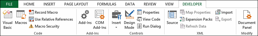
Figure 15.2. You’ll need the Developer tab to access tools specific to working with macros.

The buttons in the Code group on the Developer tab are used for recording and playing back macros:

• Visual Basic—Opens the Visual Basic Editor (VB Editor or VBE).

• Macros—Displays the Macro dialog box, where you can choose to run or edit a macro from the list of macros.

• Record Macro—Begins the process of recording a macro.

• Use Relative Reference—Toggles between using relative or absolute recording. With relative recording, Excel records that you move down three cells. With absolute recording, Excel records that you selected cell A4 (if you started in A1).

• Macro Security—Opens the Trust Center, where you can choose to allow or disallow macros to run on this computer.

Introduction to the Visual Basic Editor

Click the Visual Basic button in the Code group of the Developer tab. This will open the VB Editor, shown in Figure 15.3, which is the interface used for writing and editing macros. On the left side is the Project Explorer, which lists all the workbooks and add-ins and their components. On the right side is the Code pane, where you view and edit the macros you create.

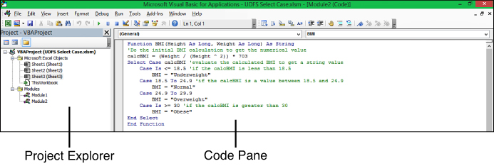
Figure 15.3. The Project Explorer on the left side of the screen is the primary method of navigating through the components of the workbook in the editor.

Project Explorer

The Project Explorer lists any open workbooks and add-ins that are loaded, as shown in Figure 15.3. If you click the + icon next to VBAProject, it becomes a - icon and opens up to show a folder with Microsoft Excel objects. There can also be folders for Forms, Class Modules, and (standard) Modules. Each folder includes one or more such components. If the Project Explorer is not visible, select View, Project Explorer from the menu.

A module is a component in the Project Explorer where you enter code. A userform, or form, is a pop-up window, for example a window that asks you to type in more information. Forms also include code.

Right-clicking a component, such as Module1, and selecting View Code or just double-clicking the desired component brings up any code in the module in the Code pane. The exception is userforms, where double-clicking displays the userform in Design view.

Inserting Modules

A project consists of sheet modules for each sheet in the workbook and a single ThisWorkbook module. Code specific to a sheet, such as controls or sheet events, is placed on the corresponding sheet. Workbook events—code that runs automatically when something happens, for example when the workbook is opened—is placed in the ThisWorkbook module. The code you record and the UDFs you create will be placed in standard modules.

To insert a standard module, follow these steps:

1. Right-click the project you need to insert the module into.

2. From the context menu, select Insert, Module.

3. The module is placed in the Modules folder.

You can insert a module from the menu by selecting the project and going to Insert, Module.

Understanding How the Macro Recorder Works

This section is about the difference between recording a macro that will run successfully on a new data set and one that will make you cry in frustration when it fails on a new data set. You’ll rarely be able to record all of your macros and have them work on different data sets, but with the tips in the following subsections, you’ll greatly improve your chances.

The macro recorder is very literal, especially with the default settings. For example, if you have cell A1 selected and then begin the macro recorder and use the mouse to select your entire data set in range A1:B10, this is what will be recorded:

Range("A1:B10").Select

If the next time you run the macro, the data set is A1:B20, your macro won’t run on rows 11–20 because the macro only covers rows 1–10. There are two things you need to change to make the recorded macro work properly. First, don’t use the mouse when selecting ranges. Second, don’t use the default settings of the macro recorder.

Navigating While Recording

To get the most out of the macro recorder, you should use keyboard shortcuts to navigate the sheet, not the mouse. The reason is that some of the keyboard shortcuts translate to commands instead of specific cell selections. For example, if you record pressing Ctrl+down-arrow to jump to the last row in a column, you will get

Selection.End(xlDown).Select

If your data set changes in size the next time you run the macro, the preceding line of code will be much more useful than if you’d recorded the macro by using the mouse. That’s because the line doesn’t mention a specific cell. Instead what it says is that, from the currently selected cell, select the last row of data before an empty cell, which is what the keyboard shortcut did.

Relative References in Macro Recording

The second rule to successful macro recording is to know when to turn relative referencing on and off. By default, it is off, which has its uses, but you’ll often want it on. You can turn relative referencing on and off as needed while recording a macro.

When relative referencing is off, the macro records specific cell addresses. Imagine you have a list of addresses similar to Figure 15.4. Each address is exactly three rows, and a blank row separates each address. To transpose an address to a single row, you would follow these steps:

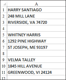
Figure 15.4. Transposing this long list of addresses to multiple columns and rows would make it easier to use them in a mail merge.

1. Start in cell A1.

2. Press the down-arrow key.

3. Press Ctrl+X to cut the address.

4. Press the up-arrow key and then the right-arrow key (to move to cell A2, remember to use the keyboard to navigate).

5. Press Ctrl+V to paste the address next to the name.

6. Press the left-arrow key once and the down-arrow key twice to move to the cell containing the city, state, and ZIP Code.

7. Press Ctrl+X to cut the city.

8. Press the up-arrow key twice and the right-arrow key twice to move to the right of the street cell.

9. Press Ctrl+V to paste the city.

10. Press the left-arrow key twice and the down-arrow key once to move to the new blank row just beneath the name.

11. Hold down the Shift key while pressing the down-arrow key twice to select the three blank cells.

12. Press Ctrl+- to bring up the Delete dialog box.

13. Press R to select the Entire Row option and then press Enter to accept the command.

If you record these steps with relative referencing off, you will get code that is cell specific, A2, B1, A3, etc., as shown in the text box in Figure 15.5. The results of running this code repeatedly on the data from Figure 15.4 are shown in Figure 15.5. A couple of repetitions of the code overwrite the first address line, ruining the record.

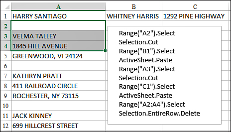
Figure 15.5. Recording the macro with relative referencing off recorded the specific cell address for processing the first address, making the code useless for subsequent addresses.

If this example was your first recorded macro, you might despair, as many before you have, at the uselessness of the recorder. But there is a way to make it work, and that’s to turn on the Use Relative References option found in the Code group on the Developer tab. Performing the same steps with relative referencing on returns the results shown in Figure 15.6. As the active (or selected) cell moves down the column, the correct fields are cut and pasted to the proper row and column.

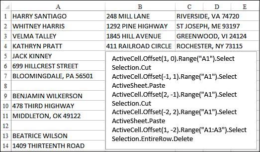
Figure 15.6. Turn on the relative reference option while recording to record your movements instead of the specific cell addresses.

Basically, if you always want the exact same cells modified, such as a header in A1:C1 that you always bold, don’t use relative referencing while recording. But if you need the flexibility of changing cell addresses, such as repeating a series of steps based on where the active cell starts, then turn on relative referencing.

Avoiding the AutoSum Button

If you use the AutoSum button while recording a macro, Excel will record the actual formula entered in the cell in R1C1 notation. It doesn’t record that you wanted it to select the range above or to the left of the formula. It’s just not that flexible. So, instead of using the AutoSum button, manually type in the formula mixing relative and absolute referencing.

For example, if you want to sum G2:G13, the AutoSum function will create the formula =SUM(G2:G13), or in R1C1 notation, =SUM(R[-12]C:R[-1]C). When viewed in R1C1 notation, you see how fixed the formula is. Although it will work in any column that it’s placed in, it specifically includes the cells 12 cells above (row 2) and directly above (row 13) the formula cell. The problem is if you add more rows, then the first cell is no longer 12 rows above—it’s more. The solution is to type in the formula manually, fixing the row for the first argument, as shown in Figure 15.7.

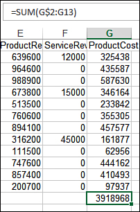
Figure 15.7. Instead of using the AutoSum button, type in SUM formulas manually, making sure to fix the row of the first argument.

Recording a Macro

To begin recording a macro, select Record Macro from the Code group of the Developer tab. Before recording begins, Excel displays the Record Macro dialog box shown in Figure 15.8. The dialog box gives you a chance to customize details about the macro, for example, replacing Excel’s generic macro name, like Macro1, with a more useful one, like FixAddressRecords.

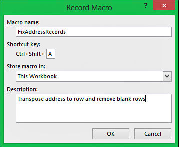
Figure 15.8. Provide details for the macro you’re about to record.

To begin recording a macro and fill in the Record Macro dialog box, follow these steps:

1. Go to Developer, Code, Record Macro. The Record Macro dialog box opens. You can also quickly access the dialog box by clicking the Record Macro button in the status bar.

2. In the Macro Name field, type a name for the macro, making sure not to include any spaces or start with a number or symbol. Use a meaningful name for the macro, such as FixAddressRecords.

3. The Shortcut Key field is optional. If you type J in this field, and then press Ctrl+J on the sheet, this macro runs. Note that most of the lowercase shortcuts from Ctrl+a through Ctrl+z already have a use in Excel. Rather than being limited to the unassigned Ctrl+J, you can hold down the Shift key and type Shift+A through Shift+Z in the shortcut box. This assigns the macro to Ctrl+Shift+A.

4. From the Store Macro In drop-down, choose where you want to save the macro: Personal Macro Workbook, New Workbook, This Workbook. It is recommended that you store macros related to a particular workbook in This Workbook.

The Personal Macro Workbook (Personal.xlsb) is not a visible workbook; it’s created if you choose to save the recording in the Personal Macro Workbook. This workbook is used to save a macro in a workbook that will open automatically when you start Excel, thereby allowing you to use the macro. After Excel is started, the workbook is hidden.

5. Enter a description of the macro in the optional Description field. This description is added as a comment to the beginning of your macro.

6. Click OK and record your macro. When you are finished recording the macro, click the Stop Recording icon in the Developer tab or in the status bar.

Running a Macro

If you assign a shortcut key to your macro, you can play the macro by pressing the key combination. Macros can also be assigned to the ribbon, the Quick Access Toolbar, forms controls, drawing objects, or you can run them from the Macros button in the Code group on the Developer tab.

Running a Macro from the Ribbon

You can add an icon to a new group on the ribbon to run a macro. This is appropriate for macros stored in the Personal Macro Workbook. Follow these steps to add a macro button to the ribbon:

1. Go to File, Options, Customize Ribbon.

2. In the list box on the right side of the dialog box, choose the tab name where you want to add the macro button.

3. Click the New Group button below the list box on the right side of the dialog box. Excel adds a new entry called New Group (Custom) to the end of the groups in that ribbon tab.

4. To move the group to the left in the ribbon tab, click the up-arrow icon on the right side of the dialog box several times.

5. To rename the group, click the Rename button. Type a new name, such as Report Macros, and click OK.

6. Open the upper-left drop-down and choose Macros from the list. Excel displays a list of available macros in the list box below the drop-down.

7. Choose a macro from the list box.

8. Click the Add button in the center of the dialog box. Excel moves the macro to the selected group in the list box on the right side of the dialog box. Excel uses a generic VBA icon for all macros, which you can change in step 9.

9. To rename or change the icon used for the macro, follow these steps:

a. Select the macro in the list box on the right side of the dialog box.

b. Click the Rename button.

c. Excel displays a list of possible icons. Choose an icon or type a new name for the macro in the Display Name field, such as Fix Addresses, as shown in Figure 15.9.

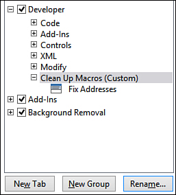
Figure 15.9. Create a custom group on the ribbon to add buttons for your macros.

d. Click OK to return to the Excel Options dialog box.

10. Click OK to close the dialog box. The new button appears on the selected ribbon tab.

Running a Macro from the Quick Access Toolbar

You can add a button to the Quick Access Toolbar to run your macro. If your macro is stored in the Personal Macro Workbook, you can have the button permanently displayed in the Quick Access Toolbar. If the macro is stored in the current workbook, you can specify that the icon should appear only when the workbook is open.

Follow these steps to add a macro button to the Quick Access Toolbar:

1. Go to File, Options, Quick Access Toolbar.

2. If the macro should be available only when the current workbook is open, open the upper-right drop-down and change For All Documents (Default) to For filename.xlsm. Any icons associated with the current workbook are displayed at the end of the Quick Access Toolbar.

3. Select Macros from the list in the upper-left drop-down, Choose Commands From. Excel displays a list of available macros in the list box below the drop-down.

4. Choose a macro from the list and click the Add button in the center of the dialog box to move the macro to the list box on the right side of the dialog box. Excel uses a generic VBA icon for all macros, which you can change by following steps 5 and 6.

5. To rename and change the icon used for the macro, follow these steps:

a. Select the macro in the list box on the right side of the dialog box.

b. Click the Modify button.

c. Excel displays a list of possible icons. Choose an icon or type a new name for the macro in the Display Name field, such as Fix Addresses, as shown in Figure 15.10. The name will appear as the ToolTip when you place your cursor over the button.

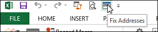
Figure 15.10. Add a button to the Quick Access Toolbar to run the macros saved to a specific workbook.

6. Click OK to close the Modify Button dialog box.

7. Click OK to close the dialog box. The new button appears on the Quick Access Toolbar.

Running a Macro from a Form Control, Text Box, or Shape

You can create a macro specific to a workbook, store the macro in the workbook, and attach it to a form control or any object on the sheet to run it. Macros can be assigned to any sheet object, such as an inserted picture, a shape, SmartArt graphics, or a text box. To assign a macro to any object, right-click the object and select Assign Macro.

Follow these steps to attach a macro to a button on a sheet:

1. In the Controls group of the Developer tab, click the Insert button to open its drop-down list. Excel offers 9 form controls (though 12 are shown, three are not usable) and 12 ActiveX controls.

2. Click the Button (Form Control) icon in the upper-left corner in the drop-down.

3. Move your cursor over the sheet; the cursor changes to a plus sign.

4. To draw a button, click and hold the mouse button while drawing a box shape. Release the button when finished and the Assign Macro dialog box opens.

5. Choose the macro from the Assign Macro dialog box and click OK. The button is created with generic text such as Button 1. To customize the text, refer to steps 6 and 7.

6. To give the button a new caption, follow these steps:

a. Right-click over the button and select Edit Text. The cursor within the button becomes visible.

b. Replace the current caption with your own text.

c. When finished, click anywhere outside the button.

7. For further text formatting options, right-click over the button and select Format Control. Click OK when done to return to Excel.

8. Click the button to run the macro.

User-Defined Functions

Excel provides many built-in formulas, but sometimes you need a custom formula not offered in the software, such as a commission rate calculator. You can create functions in VBA that can be used just like Excel’s built-in functions, such as SUM, VLOOKUP, and MATCH, to name a few. After the user-defined function (UDF) is created, a user needs to know only the function name and its arguments.

When you create a UDF, keep the following in mind:

• UDFs can only be entered into standard modules. Sheet and ThisWorkbook modules are a special type of module; if you enter the function there, Excel won’t recognize that you are creating a UDF.

• A variable is a word used to hold the place of a value, similar to an argument. Variables cannot have any spaces or unusual characters, such as the backslash () or hyphen (-). Make sure any variables you create are unique. For example, if your function is called BMI, you cannot have a variable with the same name.

• A variable type describes the variable as string, integer, long, and so on. This tells the program how to treat the variable—for example, integer and long—though both numbers have different limitations. The type also tells the program how much memory to put aside to hold the value.

• A simple UDF formula is not that different from a formula you write down on a sheet of paper. For example, if asked how to calculate the final cost of a store item, you would explain that it’s the sale price *(1 + tax rate). Similarly, in a FinalCost UDF, you might enter FinalCost = SalePrice* (1+ TaxRate), where SalePrice and TaxRate would be arguments for the function, FinalCost.

• A UDF can only calculate or look up and return information. It cannot insert or delete rows or color cells. The UDF has the same limitations as built-in functions.

Structure of a UDF

Like a normal function, a UDF consists of the function name followed by arguments in parentheses. To help you understand this, the following example will build a custom function to add two values in the current workbook. It is a function called ADD that will total two numbers in different cells. The function has two arguments, Number1 and Number2. The syntax of the function is as follows:

ADD(Number1,Number2)

Number1 is the first number to add; Number2 is the second number to add. After the UDF has been created, it can be used on a sheet.

To create a UDF in the VBE, follow these steps:

1. Open the VBE by going to Developer, Code, Visual Basic.

2. Find the current workbook in the Project Explorer window.

3. Right-click over the current workbook and select Insert, Module. A new module is added to the Modules folder.

4. Double-click the new module to open it in the Code pane.

5. Type the following function into the module’s Code pane, as shown in Figure 15.11:

Click here to view code image

Function ADD(Number1 As Long, Number2 As Long) As Long
ADD = Number1 + Number2
End Function

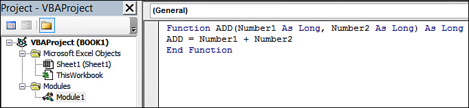
Figure 15.11. A UDF’s code must be entered in a standard module.

Let’s break this down:

• Function name: ADD.

• Arguments are placed in parentheses after the name of the function. This example has two arguments: Number1 and Number2.

• As Long defines the variable type as a whole number between –2,147,483,648 and 2,147,483,647. Other variable types include the following:

• As Integer if you were using a whole number between –32,768 and 32,767

• As Double if you were using decimal values

• As String if you were using text

• ADD =Number1 + Number2: The result of the calculation is returned to the function, ADD.

Not all the variable types in the function have to be the same. You could have a string argument that returns an integer—for example, FunctionName(argument1 as String) as Long.

How to Use a UDF

After the function is created in the VBE, follow these steps to use it on a sheet:

1. Type any numbers into cells A1 and A2.

2. Select cell A3.

3. Press Shift+F3 to open the Insert Function dialog box (or from the Formulas tab, choose Insert Function).

4. Select the User Defined category.

5. Select the ADD function and click OK. The Function Arguments dialog box opens.

6. Place your cursor in the first argument box and select cell A1.

7. Place your cursor in the second argument box and select cell A2.

8. Click OK. The function returns the calculated value, as shown in Figure 15.12.

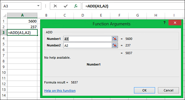
Figure 15.12. Using your UDF on a sheet is not different from using one of Excel’s built-in functions.

Sharing UDFs

Where you store a UDF affects how you can share it:

• Personal.xlsb—If the UDF is just for your use and won’t be used in a workbook opened on another computer, you can store the UDF in the Personal Workbook.

• Workbook—If the UDF needs to be distributed to many people, you can store it in the workbook in which it is being used.

• Template—If several workbooks need to be created using the UDF, and the workbooks are distributed to many people, you can store it in a template.

• Add-in—If the workbook is to be shared among a select group of people, you can distribute it via an add-in. For more information on add-ins, refer to the VBA book mentioned at the beginning of this chapter.

Using Select Case to Replace Nested IF

A really useful application of a UDF is with a Select Case statement. A Select Case statement is similar to a nested IF statement, but much easier to read. Also, because the 64 nested IF statements allowed in 2013 are not compatible in legacy versions of Excel, using a UDF with Select Case statements ensures compatibility.

The statement begins with Select Case and then the variable you want to evaluate. Next, follow the Case statements, which are the possible values of the variable, each including the action you want to take when the variable meets the Case value. You can also include a Case Else, as a catchall for any variable that doesn’t fall within the predefined cases. The statement ends with End Select.

Within the Case statements, you have the option of using comparison operators with the word Is, such as Case Is <5 if the variable is less than 5. You also have To, used to signify a range, such as Case 1 To 5.

Example: Calculate Commission

Imagine you have the following formula on a sheet. For the different type and dollar of hardware, there’s a different commission percentage to use in the commission calculation. It’s rather difficult to read and also to modify.

Click here to view code image

=IF(C2="Printer",IF(D2<100,ROUND(D2*0.05,2),ROUND(D2*0.1,2)),IF(C2="Scanner",IF(D2<125,ROUND(D2*0.05,2),ROUND(D2*0.15,2)),IF(C2="Service Plan",IF(D2<2,ROUND(D2*0.1,2),ROUND(D2*0.2,2)),ROUND(D2*0.01,2))))

Instead, take the same logic, make it a Select Case statement, and see the commission percentage breakdown for each hardware item. You can easily make changes, including adding a new Case statement. In addition, because in the original formula the commission calculation for each hardware type is the same (price*commission percentage), that formula doesn’t need to be repeated in each Case statement. Use the Select Case statements to set the commission percentage and have a single formula at the end to do the calculation. You can also provide more flexibility in case users enter a different hardware description, for example “Printers” instead of just “Printer.”

Click here to view code image

Function Commission(Hardware As String, HDRevenue As Long) As Double
Select Case Hardware 'Hardware is the variable to be evaluated
     Case "Printer", "Printers" 'If Hardware is Printer or Printers, do the following
         If HDRevenue < 100 Then 'If Hardware is less than 100
             ComPer = 0.05 'then ComPer is 5%
         Else 'else, ComPer is 10%
             ComPer = 0.1
         End If
     Case "Scanner", "Scanners"
         If HDRevenue < 125 Then
              ComPer = 0.05
         Else
              ComPer = 0.15
         End If
     Case "Service Plan", "Service Plans"
         If HDRevenue < 2 Then
             ComPer = 0.1
         Else
             ComPer = 0.2
         End If
     Case Else
             ComPer = 0.01
 End Select
 'Once a value is assigned to ComPer, do the calculation and return it to
 'the function
         Commission = Round(HDRevenue * ComPer, 2)
 End Function

Example: Calculate BMI

This example takes the user input, calculates the BMI (body mass index), then compares that calculated value with various ranges to return a BMI descriptive, as shown in Figure 15.13. When creating a UDF, think of the formula in the same way you would write it down because this is very similar to how you will enter it in the UDF. The formula for calculating BMI is as follows:

BMI=(weight in pounds/height in inches(squared)) *703

Figure 15.13. A UDF can perform calculations based on user input and return a string.

The table for returning the BMI descriptive is as follows:

Below 18.5 = underweight

18.5–24.9 = normal

25–29.9 = overweight

30 & above = obese

The code for calculating the BMI then returning the descriptive is the following:

Click here to view code image

Function BMI(Height As Long, Weight As Long) As String
'Do the initial BMI calculation to get the numerical value
calcBMI = (Weight / (Height ^ 2)) * 703
Select Case calcBMI 'evaluate the calculated BMI to get a string value
    Case Is <=18.5 'if the calcBMI is less than 18.5
        BMI = "Underweight"
    Case 18.5 To 24.9 'if the calcBMI is a value between 18.5 and 24.9
        BMI = "Normal"
    Case 24.9 To 29.9
        BMI = "Overweight"
    Case Is >= 30 'if the calcBMI is greater than 30
        BMI = "Obese"
End Select
End Function