23

Quantitative Techniques in Supply Chain

“You can use all the quantitative data you can get, but you still have to distrust it and use your own intelligence and judgment

 

—Alvin Toffler”

INTRODUCTION

Quantitative techniques are increasingly being used to find solutions to complex problems. These are used in decision-making in marketing, logistics, supply chain, operations and even in finance, when the variables are dynamic in nature, manual methods to find the solutions becomes time-consuming and error prone. For example, in the past the control of an urban expressway in Japan, has been dependent upon skilled operators’ judgement and decision. However, in 1970, the Hanshin Expressway Public Corporation started operating an automated traffic control system to maximize the total traffic flowing into its expressway network. The system relies on two control methods. The first is to limit the cars coming onto the expressway at each entrance ramp to avoid congestion in any section. The system calculates the maximum allowable inflows by solving a linear programming problem once in every 5 minutes using data from detectors installed along the expressway and at all ramps. The second method is to give drivers the most recent and accurate traffic information about the expressway and its vicinity, including expected travel times and accidents, through various information channels so that they can decide what routes to take. This system is greatly appreciated by the corporation because it is extremely cost-effective and also benefited by drivers, who now consider it an indispensable service. The linear programming using fuzzy logic solved this complex traffic congestion problem for ever.

In the process industries, a given raw material can be made into a wide variety of products. For example, in the oil industry, crude oil is refined into gasoline, kerosene, home-heating oil, and various grades of engine oil. Given the present profit margin on each product, the problem is to determine the quantities of each product that should be produced. The decision is subject to numerous restrictions such as limits on the capacities of various refining operations, raw-material availability, demands for each product, and any government-imposed policies on the output of certain products. These problems can be solved using QTs.

The application of quantitative techniques is predominant in the area of distribution, for example, there are m factories that must ship goods to n warehouses. A given factory could make shipments to any number of warehouses. Given the cost to ship one unit of product from each factory to each warehouse, the problem is to determine the shipping pattern (number of units that each factory ships to each warehouse) that minimizes total costs. This decision is subject to the restrictions that demand at each factory cannot ship more products than it has the capacity to produce.

FORECASTING

Forecasting is about predicting the future as accurately as possible. It is usually based on information available including historical data and knowledge of future events, which will have an effect on forecast. Forecasting is a statistical exercise in business, where it helps to take decisions about scheduling of production, transportation and personnel, and provides a guide to long-term strategic planning.

Modern organizations require short, medium and long-term forecasts, depending on the specific application. Short-term forecasts are needed for scheduling of personnel, production and transportation. Medium-term forecasts are needed to determine future resource requirements in order to purchase raw materials, hire personnel, or buy machinery and equipment. Long-term forecasts are used in strategic planning. Typically, businesses use relatively simple forecasting methods that are often not based on statistical modelling.

There are two broad forecasting methods such as qualitative and quantitative. ‘Quantitative’ techniques use the past data to project the future. However, the ‘qualitative’ forecasting techniques are based on the judgement of experts to forecasts. The qualitative methods are used in situations, where historical data is not available. Three qualitative forecasting methods in use are: Delphi technique, scenario writing and the subject approach.

QUALITATIVE FORECASTING

• Delphi technique: In Delphi technique, consensus of the panel experts is used in developing forecast. The methodology here is that each expert separately is asked to respond to a questionnaire. The opinions of experts are reviewed again in light of opinions of others. This process ends after some degree of consensus among experts is reached.
• Scenario writing: In this method, based on different sets of assumptions likely scenario of the business outcome are drawn out. The decision-maker has to decide which scenario is most likely to happen.
• Subjective approach: This approach calls for brainstorming exercises for employees. It allows employees to participate in the forecasting exercise. The forecasts are based on their feelings, ideas and personal experiences. New ideas to solve complex problems are thus developed. In this subjective approach, many times a survey of the company's sales people is taken.

QUANTITATIVE FORECASTING METHODS

Quantitative forecasting methods are based on an analysis of historical data. The independent variable is time and the dependent variable may be, for example, sales or profits. In this, the past data is analysed to find trends and same trend is used to forecast the future for dependent variable. In this type of forecasting method, time series on past data of the variable is used. Hence, this is called time series methods.

In the other method of forecasting along with historical data the cause-and-effect relationships of the variables is used to work out the future values of dependent variables. These forecasting techniques are called as causal methods. These methods of forecasting are used in business planning to organize resources. A few mathematical methods used for forecasting are as follows.

Correlation analysis

Correction analysis is used to measure the strength of association between quantitative variables. For example, we could measure the degree of a relationship between sales (Y) and the corresponding and spent (×). The strength of a relationship between two sets of data (sample) is usually measured by the correlation coefficient, r, where

 

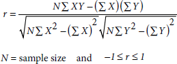
A relation is said to be perfect positive correlation when r=1 and perfect negative correlation, when r=-1. The correlation analysis is one way in measuring the variance of a simple linear regression model. There are three different types of association between variables: positive, negative or no correlation.

The following data (Exhibit 23.1) about promotional expenses and sales required to be checked for correlation.

 

 

The correlation coefficient with the above formula works out to be 0.96, which means two variables highly correlated.

Time Series Forecasting Models/Trend Exploration

Under these methods the historical data is explored to find out its cyclic nature or trends, if any. Mathematical techniques are then used to extrapolate to find out the future value/trends. The most common mathematical models in use are:

• Last period model
• Moving average model
• Weighted moving average model
• Exponential smoothing model
• Simple linear regression model (least-squares method)

Time series in general have four components such as trend, cyclical, seasonal and irregular. If these four components are combined, it provides specific values for the time series. The periodicity varies with the measurement taken at the interval of every hour, day, week, month or year.

The most popular model is linear regression model, which is suitable for the time series data that contains a trend. Linear regression is a statistical technique that expresses the forecast variable as a linear function of some independent variable. In time series modelling, the independent variable is the time period. The model (least-squares regression equation) is

 

 

where

j= forecast for dependent variable, y

x= independent variable, x, used to forecast y

â= estimated intercept term for the straight line

=b estimated slop coefficient for the straight line

 

 

(x_i, y_i)=observed values for time period i

yˉ = average y value

xˉ = average x value

n = number of observations

Once the equation of the straight line is obtained, the forecast value y can be calculated by putting in values of x.

Multiple regression is another common mathematical technique used for analysis of time series data. This model looks at the relationship between one independent variable and two or more dependent variables. Multiple regression helps to understand how a group of variables (working in unison) affect another variable.

Cross-impact matrix method   In this method, the assumption is that the occurrence of an event can, in turn, effect the likelihoods of other events. For analysis, probabilities are assigned to reflect the likelihood of an event in the presence and absence of other events. This method helps decision-makers to look at the relationships between system components, rather than viewing any variable as working independently of the others.

Scenario   The scenario is an expected forecast that is likely to happen. It describes the interrelationships of all system components. The events considered under scenario are new technology, population shifts, and changing consumer preferences. The scenario analysis enables the decision-makers to organize resources and decide course of action in advance.

Decision trees   Decision trees method is graphical representation of the structural relationships between alternative choices. The alternatives are represented as a series of yes/no choices. The decision tree structure with feedback loops is used as foundation to computer flow charts. In this, choices are assigned with probabilities to the likelihood of any particular path. The expected value of the variable/event is useful for decision-makers as it is the most likely value based on the probabilities of the distribution function.

LINEAR PROGRAMMING

A linear programming problem may be defined as the problem of maximizing or minimizing a linear function subject to linear constraints. The constraints may be equalities or inequalities. Here is a simple example. Find numbers a₁ and a₂ that maximize the sum a₁ + a₂ subject to the constraints a_j ≥ 0, a₂ ≥ 0, and

In this problem, there are two unknowns, and five constraints. All the constraints are inequalities and they are all linear in the sense that each involves an inequality in some linear function of the variables. The first two constraints, a₁ ≥ 0 and a₂ ≥ 0, are special. These are called non-negativity constraints and are often found in linear programming problems. The other constraints are then called the main constraints. The function to be maximized (or minimized) is called the objective function. Here, the objective function is aj + a₂. Since there are only two variables, we can solve this problem by graphing the set of points in the plane that satisfies all the constraints (called the constraint set) and then finding which point of this set maximizes the value of the objective function. Each inequality constraint is satisfied by a half-plane of points, and the constraint set is the intersection of all the half-planes.

Linear programming models are flexible. They adequately describe many realistic problems arising in modern industrial settings. These models take advantage of computational linear algebra that has been developed during the last 50 years. Linear programming models are largely used in logistics, transportation, finance, and warehousing, etc.

Many practical problems in operations research can be expressed as linear programming problems. The examples are network flow problem, multi-commodity flow problems which are considered important enough to have generated much research on specialized algorithm for their solutions. LP is profusely used in microeconomics and business management, either to maximize income or minimize costs of production scheme. Some other problems are food blending, inventory management, portfolio management, resource allocations for human and machine resources, planning, advertisement campaigns. LP will have the following structure:

• Defined objective with a set of decision variables.
• Defined constraints (e.g. a limited supply of resources).
• Infinite number of solutions).
• Objective and constraints are in the form of linear equations.

In linear programming, there are maximizing problems. The problem is stated with defined constraints. The problem is usually expressed in matrix form then becomes maximized. Other LP forms are minimization problems, problems with constraints on alternative forms, as well as problem involving variables can always be written into an equivalent problem in standard formats and solved through LP. LP model can be used for solving product mix problem of a firm, investment problem, scheduling problem, transportation problem and assignment problem.

Assignment Problems

Assignments problems are the ones that involve the allocation of some resources to different tasks. The objective of assignment problem is to determine the optimum assignment of given tasks to a given number of workers so that the task can be completed in minimum time. The algorithm here seeks to assign the tasks to workers in such a manner that each task will be assigned to one worker and all tasks are done in minimum time. These problems can be solved by:

• Completely enumerating all possibilities and choosing the best one.
• Drafting and solving the problem as linear (integer) programming problems.
• Solving transportation problems.
• Hungarian assignment method.

The problem is put in a matrix form. A classic example is that of airline crew members who have to be assigned to various flight schedules taking into consideration their duty hours, minimum cost of overtime and availability of flights. This problem can be solved by assignment method. These can be solved using the Hungarian method.

Another example is that of allocation of jobs to various workers for completion in optimum time.

Transportation Model

Transportation problem is a special type of linear programming problem and typically involves situation where goods are required to be transferred from some sources or manufacturing plants to some distribution centres, markets or warehouses at minimum cost. Typically in such problem a matrix is given where sources are given row wise, destinations are given column wise. The unit cost of transportation from each source to each destination is provided. The purpose is to work out dispatch schedules to reduce the shipping cost within the limitations of supply and demand quantities. The transportation can be used in other areas such as inventory control, employment scheduling and personal assignment. The transportation model can be represented as follows:

xi—quantity at supply point

yj—quantity at demand point

aij—transportation cost per unit from source to destination

bij—quantity shipped from source to destination

There are m sources and n destinations as shown in Figure 23.1. The general form of transportation problem in linear programming is as follows:

 

 

The other methods for solving transportation problems are

-Northwest corner method

-Least cost method

-Modified distribution method (stepping stone method)

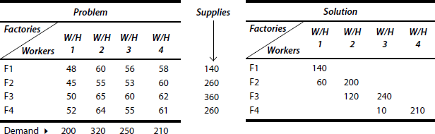
Northwest corner rule method   According to this rule, you start allocating quantities in matrix to cells from top left-hand corner cell. Allocate the maximum possible quantity in this cell to make allocation for a row/column complete. From this cell, move to the next row/column. Keep on allocating maximum possible quantities till the allocation is complete. Total number of ‘occupied cells’ must be m + n-1, where m is the number of supply centres and n, the number of demand centres.

If the number of occupied cells is less than m + n-1 the solution is said to be degenerate. In such case, assume ‘o’ (zero) allocation to a suitable cell to make occupied cells equal to m + n-1.

In the above example (Exhibit 23.2), the demand of four warehouses is fulfilled from four factories. The cost of transportation is indicated in the matrix. Logistics manager has to find out a solution for sourcing the right quantity from different factories for fulfilling warehousing demands at the optimum transportation cost. The solution is also indicated above.

 

Row minima method   Make maximum possible allocation to the minimum cost cell in a row.

Column minima method   Make maximum possible allocation column by column to the minimum cost cell in each column.

Matrix minima method   Make maximum possible allocation to the minimum cost cell and proceed in the same manner for remaining allocations.

Vogel’s approximation method (VAM)   For every row and every column, find the difference in cost between the least-cost cell and next best least-cost cell. This difference is the penalty for failing to make an allocation to the least-cost cell. Make maximum possible allocation to the row or column, where penalty is maximum. Cancel row or column for which allocation is complete and proceed in the same manner till all allocations are complete. Vogel's approximation method gives a near-optimal initial feasible solution.

Distribution method   In this method, an arbitrary initial allocation is made, and it is improved upon step-by-step till the optimum schedule is reached.

Modified distribution method (modi method)   In ‘modi’ method, the test of optimality is simplified. In this method, a set of dummy row numbers and a set of dummy column numbers are decided, and any one number is arbitrarily chosen as zero. This cell value, as mentioned earlier, is the increase in cost per unit of material transported, by making an allocation to the cell. Once the cell values are known, one can make an allocation to the cell giving maximum saving and adjusting the other allocations accordingly. The process for finding dummy numbers is a part of the test for optimality, and it is repeated for every new allocation. The negative cell value indicates incremental cost per unit, if an allocation is made to that cell. This helps in analysing the costs, if for some reason one is constrained to make an allocation to a particular cell. If the costs of making supply from a supply centre to a demand centre changes, the cell value will change accordingly. Thus, one can compute how much increase in cost per unit is allowed without making a cell-value negative. Similarly, the effect of an increase or decrease in capacity of a supply centre and effect of increase or decrease in requirement of a demand centre can be worked out by analysing changes in allocations and cell values.

ROUTE PLANNING

In a supply chain, maintaining a low-cost route structure that meets both business constraints and customer service requirements is critical to the success. In inventory movement, route planning needs to create the most efficient logistical routing plans to obtain both low cost and higher customer service. Route planning helps companies to:

• Reduce transportation costs
• Improve customer service
• Reduce cross-over miles

Route planning offers sophisticated optimization, analysis and scheduling tools for choosing among available options. It allows you to determine the optimal route mix through route schedule construction, route schedule enhancement, asset minimization, zone design, vehicle events, service technicians and dynamic sourcing.

The routing problem refers to the problem of selecting a sequence of links on a network in a particular order. In route planning, the constraints (capacity of vehicles) can be expressed as linear conditions on some appropriate variables, but can equally well be imposed on proposed solutions during a search procedure.

The route problem in logistics is commonly known as vehicle routing problem (VRP). VRP seeks to allocate some vehicles, starting at a manufacturing plant/warehouse/depot to a set of demand locations each, and minimize costs, while satisfying other constraints (typically total length of each tour or capacity constraints on vehicles). For these problems, one basic idea is to construct reasonable tours and then modify them, based on some savings by interchanging locations on the tour. This works well for many practical problems in logistics applications.

The VRP, with capacity constraints, is quite frequently encountered in practice, for example, in the weekly despatching problem in multi-product, multi-location environments, where a good service frequency is desired. It is quite often used in local or secondary movement of goods, where frequent despatches, which combine several locations, is a cost-effective option. This is very common in delivery of perishables such as milk, ice-cream, vegetables, courier operations, etc.

The other common constraint in VRPs is the time window constraint, which gives a time interval during which a certain node must be visited. This makes optimal routing more difficult to obtain.

A routing problem for which an exact solution is easily available is the so-called shortest path problem. This is to find a sequence of nodes (from a given origin to a given destination) on a network for which the total cost is minimum. This can be done by a constructive procedure such as the well known Dijkstra's algorithm. Finding the shortest path for all origin-destination pairs turns out also to admit an efficient procedure (e.g., Floyd's algorithm).

A problem which is perhaps peculiar to India is the Indian truck routing. The simplest version of this is to find a set of paths so that each path begins at a given root node, all the nodes in the network are covered by the paths and the sum of all the path lengths is minimized. The root node refers to the factory or the dispatching points and the other nodes are the demand locations.

QUEUING THEORY

The queuing theory is an important tool used to find solutions to supply chain problems. It is used to study situations in which customers (or orders placed by customers) form a line and wait to be served by a service or manufacturing facility. Clearly, long lines result in high response times and dissatisfied customers. The queuing theory may be used to determine the appropriate level of capacity required at manufacturing facilities and the staffing levels required at service facilities, over the nominal average capacity required to service expected demand without these surges. Any business process where lines are a matter of fact, queuing theory is used. Examples are as follows:

• Doctors’ clinics
• Restaurants
• Server load in a network environment
• Fulfilment/distribution centre or warehousing
• Project management
• Call centres

Queuing solution is suitable for solving a service-oriented problem where customer arrives randomly to avail of the service. The queuing model is relevant in service-oriented industries such as logistics, transportation, shipping, hospitality, banking, etc. The key elements of the process are given here.

Source Customers

Source involves a finite or limited number of customers. In a telephone system there is a large source population. When there are more than 100, the source can be treated as if it is infinite in size and the number of potential customers will influence the arrival behaviour of customers for the service system.

Arrival Process

The customer will reach the service system as per their needs. Many customers may arrive in batches (e.g. family) or individually. Customers may also arrive on a scheduled basis (e.g. appointment with manager). The customer arrival process describes the behaviour in which customers reach the service system. Arrival process is measured either by arrival rate numbers per hour or inter arrival, for example, each visiting every 15 minutes. When service is provided on a scheduled basis, the arrival rate or inter-arrival time is fixed. In unscheduled situations, however, customers arrive in a random pattern. The random pattern in most queuing situations follows the Poisson distribution.

Waiting Line

Customers do not physically form a queue but the queue is formed in the booking at their arrival in the system. The important factors to consider in a queuing system are size or capacity of the waiting area (customers may turn away if it is full), queue length (customers may refuse to join if it is too long) and queue organization (customers may refuse to join the queue if the queue is not organized).

Queue Discipline

The method in which customers from the waiting area are selected for service is referred as the queue discipline. The following are queuing disciplines which can be followed:

• First-in-first-out (FIFO)
• Last-in-first-out (LIFO)
• Priority scheme

Service Process

The simplest case is a single service facility while others may consist of multiple servers in one stage or multiple stage servers. Following are some examples:

• Single server, single stage
• Multiple servers, single stage
• Multiple parallel, non-identical servers, single stage
• Single server, multiple stage
• Multiple server, multiple stages

Regardless of the design configuration, it will take time to perform the service at each server. There are two ways to describe this service process, as follows:

• Service rate—The number of customers served per unit of time, for example, 30 per hour.
• Service time—The time taken to serve a customer, for example, 2 minutes per service.

Service time may be constant (e.g. machine processing) or may fluctuate (e.g. check out point in a supermarket) within some range of value. We can use probability distribution (e.g. negative exponential distribution) to describe the service process if it is fluctuating.

Departure

Most customers may return to the queuing system after servicing while others may never return again.

There are several measurements that should be considered when measuring the performance of a queuing system. However, the average value of the following listed measurements for a system is in a steady state which needs to be calculated.

λ—Average arrival rate

µ—Average service rate

ρ—System utilization

LS—Average number of customers in the queuing system

Lq—Average number of customers in the waiting line

WS—Average time a customer spends in the system

Wq—Average time a customer spends in the waiting line

Pn—Probability of there being n customers in the queuing system

There are two types of queuing systems: transient state (where probability of the number of customers in the system depends upon time) and steady state (where probability of the number of visiting customers in the system is independent of time).

A single queue single server model is represented—(M /M /1 /∞/∞) Wherein:

 

 

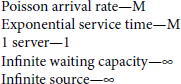
The assumptions here are: unlimited customers, unlimited waiting area. First-come-first-served, single server, arrival rate follows a Poisson distribution, and service time follows a negative exponential distribution. The formula calculations are:

 

 

For example, a petroleum company distributes its products by tankers loaded at its only loading station. Both company's and contractor's tankers are used for this purpose. It was found that on an average every 7 minutes one truck arrived and the average loading time is 5 minutes; 40 per cent trucks belong to contractors. Using queuing model and by making certain assumptions, one can find out the probability that a truck has to wait before loading, etc.

A queuing system is a model with the structure such as customers arrive and join a queue to wait for service given by n servers, after receiving service, the customer exits the system. A fundamental result of queuing theory is ‘Littles law’. For a queuing system in steady state, the average length of the queue is equivalent to the average arrival rate multiplied by the average waiting time.

For example, consider a warehouse with 5, 000 pallets of product that turns @4 times per year. Does it have enough labour to support these transactions? We get

 

 

Assuming a 10-hour shift per day of about 250 working days per year, there is roughly 2, 000 working hours.

then, ρ= 10 pallets/hour

The above analysis helps to estimate the labour force required to move pallets, receive product, move product, and get work done.

In addition to the above, in general there are many more applications of queuing theory which show the interplay between the arrival rate and the service rate, which both reveal the characteristics of the queue and, ultimately the customer experience.

SIMULATION

Simulation is used to study situations characterized by uncertainty. Simulation involves the creation of a model of a system based on specific assumptions about system behaviour and information about probability distributions associated with various variables. By running simulations, it may be possible to determine the best values of various system parameters, in context with underlying assumptions. The main advantage of simulation is that it can be used to study extremely complex systems that cannot be easily modelled by using other mathematical tools. According to T. H. Taylor:

Simulation is a numerical technique for conducting experiments on digital computers, which involves certain types of mathematical and logical relationships necessary to describe the behaviour and structure of a complex real world system over extended period of time.

Simulation is a procedure whereby one can draw conclusions about the behaviour of a given system by examining the behaviour of a corresponding model whose cause and effect relationships are similar to those in the actual system. Simulation provides trial and error method towards optimal solution. Simulation is a quantitative method, wherein a mathematical model would represent the interrelationships between the variables involved in the actual situation in which a decision is to be taken. Then, a number of experiments are conducted with the model to determine the results that can be expected when the variables assume various values.

Simulation can serve as a ‘pre-test’ to try out new decision rules for a system. Simulation can anticipate problem and bottlenecks that may rise while operating a system. There are a few basic concepts which must be understood before applying the simulating technique.

• System: It is that segment to be studied or understood to draw conclusions. In the product-market system, the market for the products together with the firm's production process constitutes the relevant system. The variable can be identified only after defining the system. These are the variables, which interact with one another in the system and establish their relationships mathematically.
• Decision variables: Decision variables are those variables whose value is to be determined through the process of simulation.
• Environmental variables: These are the variables which describe the environment. In marketing, competitors’ average price, consumer preferences and demand, etc. are the environmental variables.
• Endogenous variables: These variables are generated within the system itself. In marketing, quantity sold, sales revenue, total cost and profit are endogenous variables.
• Criterion function: Any variable can be used as the criterion function for evaluating the performance of the system. In marketing, profit is used as the criterion function.

Mathematical modelling requires the setting up of mathematical relationships which would represent the system. While some relationships can be expressed as equations, other relationships or constraints on the criterion function may be expressed only as inequalities (as we have seen in linear programming). If the mathematical model set up could always be optimized by the analytical approach, then, there would be no need for simulation. Only when interrelationships are too complex or there is uncertainty regarding the values that could be assumed by the variables or both, we would have to resort to simulation. In the complex interrelationship situation, ‘Monte Carlo’ method is a technique that involves using random numbers and probability to solve problems. The term ‘Monte Carlo’ method was coined by S. Ulam and Nicholas Metropolis in reference to games of chance, a popular attraction in Monte Carlo, Monaco.

Computer simulation has to do with using computer models to imitate real life or make predictions. When you create a model with a spreadsheet like Excel, you have a certain number of input parameters and a few equations that use those inputs to give you a set of outputs (or response variables). This type of model is usually deterministic, meaning that you get the same results no matter how many times you re-calculate.

Monte Carlo simulation is a method for alliteratively evaluating a deterministic model using sets of random numbers as inputs. This method is often used when the model is complex, non-linear, or involves more than just a couple uncertain parameters. A simulation can typically involve over 10, 000 evaluations of the model, a task which in the past was only practical using super computers.

By using random inputs, you are essentially turning the deterministic model into a stochastic model. Monte Carlo simulation is categorized as a sampling method because the inputs are randomly generated from probability distributions to simulate the process of sampling from an actual population. So, we try to choose a distribution for the inputs that most closely matches data we already have, or best represents our current state of knowledge. The data generated from the simulation can be represented as probability distributions (or histograms) or converted to error bars, reliability predictions, tolerance zones and confidence intervals.

GAME THEORY

Game theory (GT) is a powerful tool for analysing situations in which the decisions of multiple agents affect each agent's payoff. As such, GT deals with interactive optimization problems. GT may be used to model negotiation processes in supply chains and to develop insights into the balance of power in supply chains. Enterprises can be seen as players in a game defined by a common goal, but has separate constraints and conflicting objectives. In order to obtain acceptable trade conditions, a certain form of negotiation turns out to be necessary. GT provides a mathematical background for modelling the system and generating solutions in competitive or conflicting situations. The basic rationality principle of game theory states that each player acts to optimally accomplish his/her individual goal, taking into account that the others play in the same manner. However, if the individual goal of each player is uniquely to maximize his gain or to minimize his loss, the agreements obtained by negotiation may be fragile and will not generally guarantee enterprise optimality for the whole supply chain, particularly when external demand is stochastic. For these reasons, much effort has been recently devoted to conceiving contracts strengthening the commitments of partners through risk, profit or cost sharing, and/or moving the equilibrium state of the game towards a better global performance. Examples of contract parameters that can be used to achieve coordination, are quantity discounts, returns (buy backs), quantity flexibility, and the use of subsidies/penalties.

Cooperative GT can be of great help to design a supply chain or a virtual enterprise by selecting an optimal coalition of partners. But a non-cooperative (also called strategic) approach is certainly more appropriate to determine the set of equilibrium points that can be reached in trade conditions. A case of particular interest is when there exist decisional states from which neither player has interest to depart. Such cases, called Nash equilibria, have received a considerable attention both in theory and applications of GT. A particular property of a Nash equilibrium point is that, if the internal models of the players are known it is immediately reached at the first iteration of the game. Therefore, existence of Nash equilibrium points reduces the negotiation process to a one-shot exchange of information. In many real situations, the equilibrium is not unique, and the first player imposes the outcome of the game. The particular equilibrium reached in such an asymmetric game is called ‘Stackelberg equilibrium’. Outside the full information context, the outcome of a game generally depends on who plays first and how the players negotiate.

In enterprise networks, decentralized decisions are generally less efficient than a centralized mechanism maximizing a global utility function. In particular, when decisions are decentralized with different utility functions, a system with a dominant actor usually leads to a Stackelberg game in which the leader gets the maximal value of his/her utility function while the followers are maintained at their minimal acceptable satisfaction level. However, in spite of this unbalance, such an equilibrium may correspond to global optimal conditions, provided that the contracts between the partners allow for a shift of local equilibria toward globally optimal values. In this respect, different contracts have been shown to possess this property delay adjustment mechanisms for retail prices, delay dependent prices for delivery from the supplier.

Thus, GT has become an essential tool in the analysis of supply chains with multiple agents, often with conflicting objectives.

MODELLING

A model usually refers to a particular ‘level in the managerial decision making’ context and the decisions of the higher levels. For example, an operational model will have certain constraints imposed by a tactical level decision. Mathematical modelling is probably most useful for tactical decision-making, with a certain time horizon and where certain level of aggregation of data is possible. For higher level decision-making, wherein data is uncertain and intangibles are many, the hard modelling is not useful for the most part. Other ones, such as soft systems modelling, some models of discrete decision analysis and cognitive maps are possibilities for strategic decision-making. In all modelling the quantification of certain key elements of cost, or quantifying the attributes of various scenarios, is often very useful in strategic decision-making process.

Models are useful to describe the inter-relationships between different quantities of interest and sometimes to derive certain optimal or good policies. The models based on mathematical programming, inventory theory, routing and scheduling theory can directly address a sharp decision area, or can be part of the quantitative assessment for more aggregate decisions. For many strategic decisions, a generalized approach called ‘alternatives assessment, which works through the consequences of a limited number of possibilities or alternatives is good enough.

Inventory Models

Inventory (stocks) is an inevitable integral part of every business operation. Inventories occur in all forms and for the most diverse purposes. In applications involving inventory, manager must answer two important questions: How much should be ordered? When to order?

The EOQ or economic lot size model is referred as Wilson-Harris square root formula since it was devised by Ford Harris and R. H. Wilson independently. The assumptions under this model are as follows:

• Demand is known. It is constant and over spread uniformly over a period of time.
• No lead-time for re-supply of material and material is supplied instantaneously.
• The cost of ordering per unit is same irrespective of the lot size.

In this model, inventory-carrying cost may be taken to be proportional to the average inventory held during a period. Therefore, by reducing the inventory, its carrying cost can be reduced. On the other hand, the smaller lot size will increase the number of lot sizes per year to cover the annual demand and hence, the cost of ordering will be more. Hence, economic lot size will have to balance these two opposite costs.

The mathematical formula for economical lot size is

 

 

where Q=Economic order quantity in units

        S=Cost of placing an order in Rs

        D=Average annual consumption in units

        H=Percentage of inventory cost vis-à-vis unit cost

        C=Cost per unit

The formula is based on certain assumptions, which in practice is not relevant. These are:

• Standard pack size available in the market forces buyer to modify EOQ.
• EOQ may be modified if seller offers the quantity discount.
• The ordering quantity in practice is based on funds availability and may compel the buyer to buy less than EOQ.
• Higher quantities may be ordered to take care of the future shortage of material in the market.

The EOQ formula is a guideline for the decision-makers and can be used with deviations in light of the practical limitation.

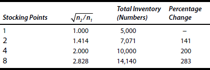
Square Root Law

This law was formulated by Maister in 1976 to minimize the risk in inventory carrying at multiple placing. It is done for risk pooling and inventory centralization. This law in the form of a formula calculates the benefit obtainable by inventory centralization. The formula is

 

 

where n₁= number of existing facilities

     n₂= number of future facilities

     x₁= total inventory in existing facilities

     x₂= total inventory in future facilities

Exhibit 23.4 demonstrates how average inventory level increases as the number of stocking locations increase.

 

 

SRL is based on the following assumptions:

• No inventory transfer between stocking locations.
• No variations in the lead-time.
• Uniform customer service level.
• Demand at each location is normally distributed.

The limitation to SRL is its effectiveness, when the demands across the markets are served by the various stocking points. SRL will be most effective when markets have demands, which are negatively correlated and there is little or no benefit from consolidation when demands faced by the various stocking points are positively correlated. Additionally, the more the uncertainty of demand at each location, measured by the coefficient of variation, the better the SRL of inventory works.

Warehouse: Cost vs Area

Bowman-Stewart formula explains the relation between the cost of warehouse operation and optimum area served by the same. The thumb rule is that the supply point be near to the demand points. This means the warehouse location should be in proximity to the market. There is no limitation to the area of the warehouse for serving the particular market. However, the logistics cost goes up with the distance between warehouse and the place of delivery. As per Bowman-Stewart formula, the cost of delivery is proportional to the square root of the area covered by the stocking point. This can be expressed as:

 

 

The choice of location is decided on the cost of delivery. The other variable affecting the cost is sales off-take. If cost of delivery is, say, A and B is sales volume for a given time period, then A/B is cost per unit sales, which is part of total cost element of the warehouse. Considering the fixed cost of the warehouse as F, the total cost of warehouse operation shall be expressed as:

 

 

The formula can be further refined by introducing the sales density ‘D’, that is defined as sales per unit area (geographical) served by the particular warehouse.

 

 

For optimizing the cost, the total cost function has to be differentiated with respect to warehouse area S.

 

 

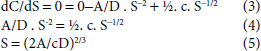
The warehouse service area can be found out by knowing the variable cost related to sales volume ‘A, the sales density ‘D’ and the cost of ‘c’ delivery. For higher cost of warehouse operation, the warehouse service area needs to be enlarged, and in case of increase in servicing cost, servicing the area needs to be reduced for optimization.

LIMITATIONS OF MATHEMATICAL MODELS

Any mathematical model of a supply chain rests on assumptions about the supply chain. The outcome obtained is only as good as the assumptions and the model. The recommendations obtained from any mathematical model must be tested for sensitivity to the underlying assumptions and the underlying assumptions must be thoroughly tested for reasonableness.

It is also important to realize that mathematical models can only provide answers to questions posed by a decision-maker. The task of asking the right questions and identifying the underlying problems facing a firm cannot be performed by a mathematical model. For instance, a sophisticated procedure for the routing of vehicles will not significantly benefit a firm that is selling the wrong set of products or is using the wrong set of suppliers. Supply chain mathematics cannot act as a substitute for intelligent decision-making by managers.

REVIEW QUESTIONS

1. Find out the different application areas of quantitative techniques and discuss the role of quantitative techniques in supply chain.
2. Discuss the applications of ‘linear programming (LP)’ in logistics.
3. Explain with illustrations how queuing theory is used in logistics supply chain optimum servicing rate and optimum cost.
4. What is modelling? Explain how it is useful in supply chain optimization.

INTERNET EXERCISES

1. Read more on forecasting—advantage, type, cost, practical applications, methods, http://www.refer-enceforbusiness.eom/small/Eq-Inc/Forecasting.html#ixzz0oZxuwv7f http://enceforbusiness.eom/small/Eq-Inc/Forecasting.html%23ixzz0oZxuwv7f
2. For queuing problems and solutions visit http://www.shmula.com/91/queueing-theory-part-1#ixzz0n2ns47MK and http://www.shmula.eom/117/queueing-theory-part-2#ixzz0n2oLyvQP http://www.shmula.eom/117/queueing-theory-part-2%23ixzz0n2oLyvQP
3. Visit http://www.profit.com and study ‘Optimizing Routing and Transportation’ using software.
4. Visit http://www.opsresarch.com for studying more on vehicle routing and modelling.
5. Find out if there is relationship between the ‘economic batch quantity’ and the ‘Kanban quantity.

VIDEO LINKS

1. Transportation problem http://wn.com/Profribasmat217
2. Linear programming optimisation http://wn.com/Profribasmat217

PROJECT ASSIGNMENT

1. Manufacturing companies are maintaining multiple warehouses in different states in India and due to current CST rules to reduce tax incidence. With new GST implementation, the companies will reduce the number of warehouses to reduce the operation cost. Select a company with multiple warehouses and use appropriate QT to decide the optimum number of warehouse to extend present level of service level.