
Chapter 7 - Denormalization
“Insanity: doing the same thing over and over again and expecting different results.”
Denormalization
A Teradata data warehouse is designed to utilize a Third Normal Form model, but there are thousands of users and often thousands of databases and tables. For performance reasons, after the model is complete and access and tendencies are understood, denormalizing can be a benefit.
Here are the fundamental denormalization techniques:
- Derived Data
- Repeating Groups
- Pre-Joins
- Summary and/or Temporary Tables
- Partitioning (Horizontal or Vertical)
Make these choices AFTER completing the Logical Model.
- Keep the Logical Model pure and untainted.
- Keep the documentation of the physical model current.
I was discussing denormalization with the mastermind of the largest data warehouse in the world. He mentioned that they denormalize, and I asked him why. He said, “We have users doing the same thing thousands of times a day, so it saves us enormous time and money.” That is the real reason you would denormalize.
Derived Data
The key factors for deciding whether to calculate or store stand alone derived data are:
• Response Time Requirements
Response Time Requirements – Derived data can take a period of time to calculate while a query is running. If user requirements need speed, and their requests are taking too long, then you might consider denormalizing to speed up the request. If there is no need for speed, then be formal and stay with normal.
• Access Frequency of the request
Access frequency of the request – If one user needs the data occasionally, then calculate on demand, but if there are many users requesting the information daily, then consider denormalizing so many users can be satisfied.
• Volatility of the column
Volatility of the column – If the data changes often, then there is no reason to store the data in another table or temporary table. If the data never changes, and you can run the query one time and store the answer for a long period of time, then you may want to consider denormalizing.
Repeating Groups
Sales_Table at one of the largest data warehouses in the world showing Daily_Sales
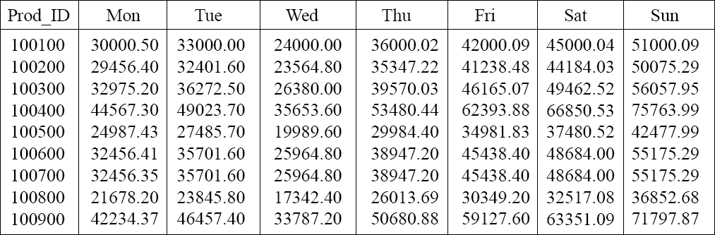
The above table actually saves space because, if the table did not use repeating groups, there would be 7 times the rows and 14 extra bytes of row overhead per row. Instead of 150,000 rows, this table would have over 1 million rows.
The above table is not about saving space. The customer needs to compare how Monday did versus Tuesday, etc. This table allows users to get the information about a product during a specific week by reading only one row and not seven. Although this violates first normal form, it can be a great technique for known queries.
Pre-Joining Tables
Employee and Department Table Denormalized into one table

| Dept_No | Department_Name | Budget |
| 100 | Marketing | 500000.00 |
| 200 | Research and Develop | 550000.00 |
| 300 | Sales | 650000.00 |
| 400 | Customer Support | 500000.00 |
Pre-Joining tables makes sense if thousands of times a day they are joining.
Storing Summary Data with a Trigger
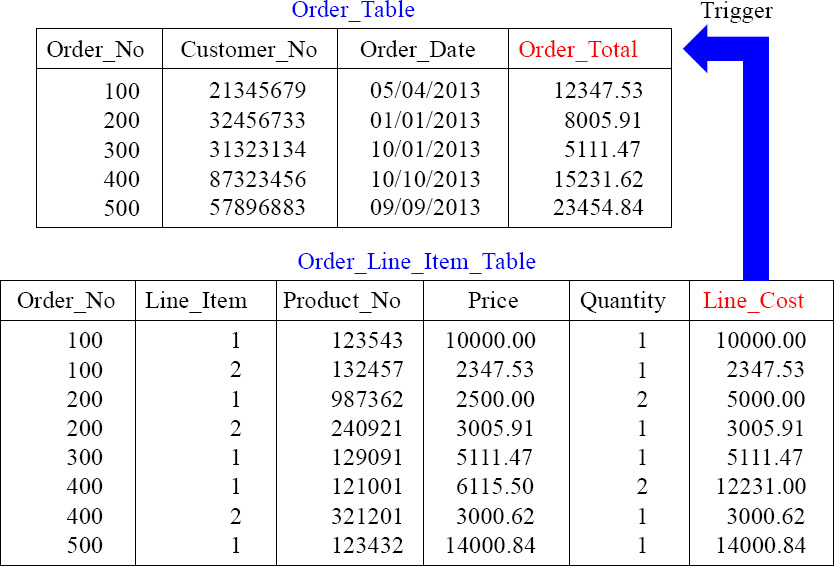
To keep the Order_Total updated in the Order_Table, a TRIGGER adds or subtracts the Order_Total when a line item is added or subtracted from the Order_Line_Item_Table.
Summary Tables or Data Marts the Old Way
Call_Billing_Monthly_Table
| Customer_No | Call_Date | Cost |
| 1 | 01/01/2013 | 1.53 |
| 2 | 01/01/2013 | 2.91 |
| 3 | 01/01/2013 | 3.70 |
| 1 | 01/01/2013 | 0.12 |
| 2 | 01/01/2013 | 11.50 |
| 3 | 01/01/2013 | 12.91 |
| • | • | • |
| • | • | • |
Billions of rows
Call_Billing_Data_Mart
| Customer_No | Total_Owed |
| 1 | 1.65 |
| 2 | 14.41 |
| 3 | 16.61 |
| • | • |
| • | • |
Thousands of rows
Each night, the Call_Billing_Monthly_Table builds the data mart holding the summary data. Now if a customer calls the call center, employees can quickly discuss their bill.
Aggregate Join Index the New Way
CREATE JOIN INDEX Agg_Order_IDX AS SELECT
Customer_Number
,Extract(Year from Order_Date) As Yr
,Extract(Month from Order_Date) As Mon
,Count(*) as County
,Sum(Order_Total) as Summy
FROM Order_Table
Group by 1, 2, 3 ;
Only Sum and Count can be used with an Aggregate Join Index.
Teradata can utilize an Aggregate Join Index. Now, your Sum and Counts are always available, and anytime the base table is updated so is the join index. Users never query the Join Index directly, but the Parsing Engine commands the AMPs to pull the data from the Join Index when appropriate. Now, you can keep your normalized model, won't need to build a data mart, and still have the data almost instantaneously.
New Aggregate Join Index (Teradata V14.10)
CREATE JOIN INDEX Agg_Order_IDX AS
SELECT
Customer_Number
,Extract(Year from Order_Date) As Yr
,Extract(Month from Order_Date) As Mon
,Count(*) as County
,Sum(Order_Total) as Summy
,MAX (Order_Total) as Max_Ord
,MIN(Order_Total) as Min_Ord
FROM Order_Table
Group by 1, 2, 3;
Only Sum and Count can be used with an Aggregate Join Index (pre Teradata V14.10).
Now Min and Max can be used with an Aggregate Join Index (Teradata V14.10).
Aggregate Join Index (AJI) has always supported (SUM and COUNT), but with Teradata V14.10, there is support for MIN/MAX aggregates also.
Horizontal Partitioning the Old Way
Order_Table with Trillions of Rows
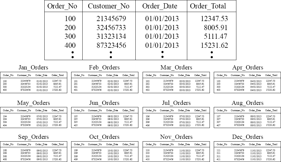
We have taken the Order_Table with Trillions of rows and have broken it into 12 separate monthly Order tables to speed up queries on different months. That is the old way.
Horizontal Partitioning the New Way
Order_Table with Trillions of Rows
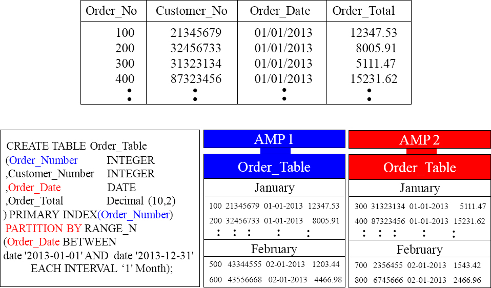
Teradata has Partitioned Primary Index (PPI) tables that allow you to partition rows.
Vertical Partitioning the Old Way
Table_Wide_Column has 300 Columns
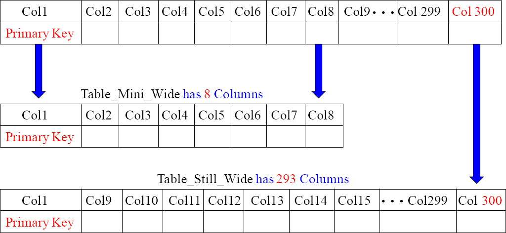
We have taken a table with 300 columns and split it into two tables. The first table contains the eight columns users query the most. The second table has the same Col1 (Primary Key) and the remaining 292 columns that aren't queried that often. We can still join the two tables if we need more than just the first eight columns. That is the old way of doing it. Turn the page and see the new way.
A Vertical Partitioning Trick that is Old School
Table_Wide_Column has 300 Columns

CREATE UNIQUE INDEX Sec_IDX (Col1, Col2, Col3, Col4, Col5, Col6, Col7, Col8) ON Table_Wide_Column ;
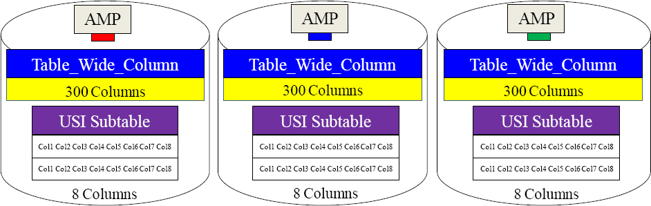
We created a multi-column Unique Secondary Index (USI) containing the first eight columns. When users query only the first eight columns, the PE will command the AMPs to get the data from the USI subtable. This is called a cover query.
Vertical Partitioning the New Way
Table_Wide_Column has 300 Columns

Teradata now has Columnar Tables that partition the columns vertically into their own separate containers. This is designed to move less blocks into FSG Cache when users only query a few columns. Each column has its own separate block (container). Each AMP still holds 300 columns (the entire row), but each column is separated in its own block. So, when users query the first eight columns, only a little of the data moves.
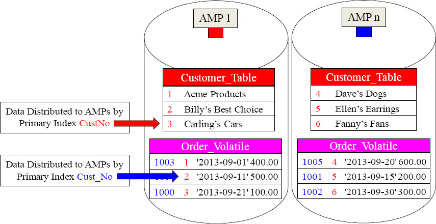
Temporary Tables - A Volatile Table with a Primary Index

It is a great idea to give your Volatile Table a Primary Index so you can control how it is distributed and the best way you want to query it. In the above example, we knew we wanted to join this to another table. So we made the Primary Index the join condition.
The Joining of Two Tables Using a Volatile Table
SELECT C.CustNo,
,C.CustName
,V.Order_Total
FROM Customer_Table as C
INNER JOIN Order_Volatile as V
ON C.CustNo = V.CustNo ;
We gave our Volatile Table a great Primary Index fully knowing we were going to populate it with September orders, and then join it to the Customer_Table on the join condition of CustNo. Now, no data movement is required. Brilliant!
Temporary Tables - Global Temporary Tables

CREATE Global Temporary TABLE Order_Global
( OrderNo Integer NOT NULL
,CustNo Integer
,Order_Date Date COMPRESS
,Order_Total Decimal(10,2) COMPRESS
) Primary Index (CustNo)
ON COMMIT PRESERVE ROWS ;
Give your Global tables a Primary Index, and use the Keyword COMPRESS for any column that is Nullable and NOT the Primary Index.

INSERT INTO Order_Global
SELECT OrderNo, Cust_No,
Order_Date, Order_Total
FROM Order_Table
WHERE
extract(Month from Order_Date) = 9 ;
Any user with Temp Space can materialize the table with an Insert/Select Statement, and the data won't be deleted until they logoff.

SELECT * FROM Order_Global
ORDER BY 1;
The data is deleted when the user does logoff, but the table structure stays permanently.
Give your Global Temporary Tables a Primary Index and also compress any Nullable column. If a null is present, then Teradata will compress it and save space.
The Joining of Two Tables Using a Global Temporary Table
SELECT C.CustNo,
,C.CustName
,G.Order_Total
FROM Customer_Table as C
INNER JOIN Order_Global as G
ON C.CustNo = G.CustNo ;
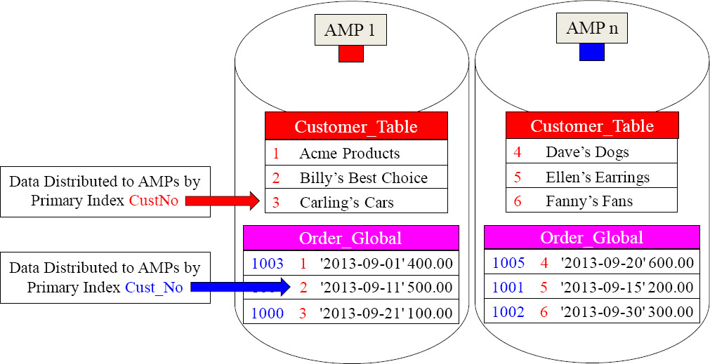
By giving the Global Temporary Table a Primary Index of CustNo the matching rows are on the same AMPs.
We gave our Global Temporary Table a great Primary Index fully knowing we were going to populate it with September orders, and then join it to the Customer_Table on the join condition of CustNo. Now no data movement is required. Brilliant!
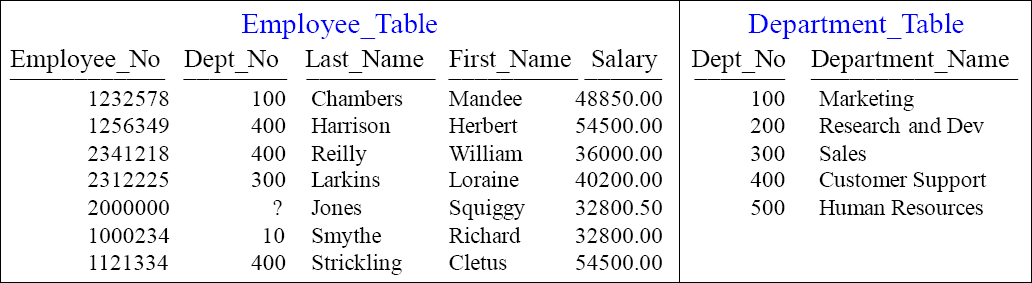
Creating a Multi-Table Join Index
CREATE JOIN INDEX EMP_DEPT_IDX AS
SELECT Employee_No
,E.Dept_No
,First_Name
,Last_Name
,Salary
,Department_Name
FROM Employee_Table as E
INNER JOIN
Department_Table as D
ON E.Dept_No = D.Dept_No
PRIMARY INDEX (Employee_No) ;
The Syntax above will create a Multi-Table Join Index with a NUPI on Employee_No. The next slide will illustrate a visual so you can see the data in the Join Index. Join Indexes are created so data doesn't have to move to satisfy the join. The Join Index essentially pre-joins the table, and keeps it hidden for the Parsing Engine to utilize.
Visual of a Join Index
Join Index named EMP_DEPT_IDX
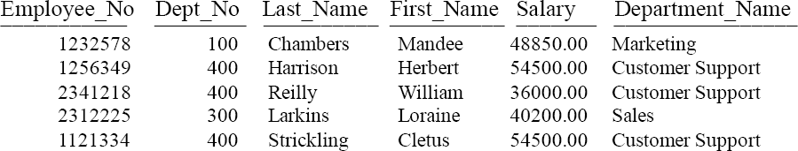
The Join Index looks like an Answer Set, but each row is stored like a normal table. The rows of the Join Index are spread amongst the AMPs. Users can't query the Join Index, but the Parsing Engine gets data from the Join Index when it chooses. A Join Index is used for speed because no data is actually joined or redistributed.
Creating a Single-Table Join Index
CREATE JOIN INDEX Employee_IDX
AS
SELECT Employee_No
,Dept_No
,First_Name
,Last_Name
,Salary
FROM Employee_Table
PRIMARY INDEX (Dept_No) ;
We've duplicated the Employee_Table with a different Primary Index.
If a USER queries with the Dept_No in the WHERE clause, this will be a Single-AMP retrieve. If the USER joins the Employee and Department Tables together, then Teradata won't need to Redistribute or Duplicate to get the data AMP local. The next page will give you a visual of how that looks on a particular AMP.
Conceptual of a Single Table Join Index on an AMP

Notice the Primary Indexes on both tables and the Single Table Join Index. The Join Index gives the Parsing Engine options. If a query is run against the Employee_Table with Employee_No in the WHERE clause, it will use the normal table. But, if a user Uses Dept_No in the WHERE clause it will use the Join Index. If a user needs to join the Department_Table to the Employee_Table, the Join Index is used so no data moves.
Single Table Join Index Great For LIKE Clause
Build a STJI with column that contains three columns. They are the LIKE column being queried, the primary index column of the base table and the keyword ROWID!
CREATE JOIN INDEX Good_For_Like AS
SELECT License_Plate, PI_Col, ROWID/* Global Join Index */
FROM BMV_Table
Primary Index (PI_Col) ;
SELECT *
FROM BMV_Table
WHERE License_Plate LIKE ‘TeraT%’ ;
The PE will choose to scan the narrow table (the Join Index) and qualify all rows that qualify with a car license LIKE ‘TeraT%’, then the PE uses the ROWID to get data from the BMV_Table where row is on the same AMP because both the base table and join index are on the same AMP because they both have the same Primary Index. This can save enormous time for queries using the LIKE command.
A LIKE command on a base table will never use a Non-Unique Secondary Index (NUSI). The above technique should be tested and only used if a lot of users are utilizing the LIKE command on a large table. If that is the case a lot of time can be saved.
Single Table Join Index with Value Ordered NUSI
A Value Ordered NUSI can only be done on columns that are 4-byte integers. Dates qualify because they are stored internally in Teradata as 4-byte integers.
CREATE JOIN INDEX OrdersJI AS
Select * from Order_Table
Primary Index(Customer_Number) ;
Create Index (Order_Date) order by values on OrdersJI;
A value ordered index has been expanded from 16 to 64 columns.
Indexes are always sorted by their hash, but a Value Ordered index is sorted on each AMP by values and not hash. This is a great technique for you to run trials on.
Sparse Join Index
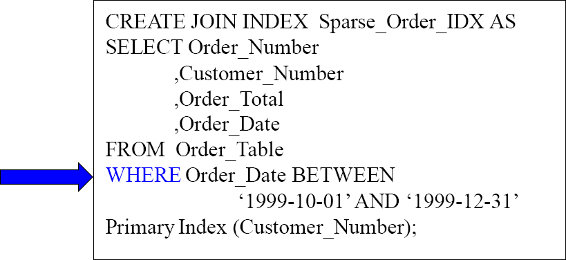
A Sparse Join Index is a Join Index with a WHERE Clause!
A Sparse Join Index has a WHERE clause so it doesn't take all the rows in the table, but only a portion. This is a very effective way to save space and focus on the latest data.
A Global Multi-Table Join Index
CREATE JOIN INDEX EMP_DEPT_Glob
AS SELECT Employee_No
,E.Dept_No
,First_Name
,Last_Name
,E.ROWID as EmpRI
,Department_Name
,D.ROWID as DeptRI
FROM Employee_Table as E
INNER JOIN
Department_Table as D
ON E.Dept_No = D.Dept_No
PRIMARY INDEX (Dept_No) ;
With the ROWID inside the Join Index, the PE can get columns in the User's SQL NOT specified in the Join Index directly from the Base Table by using the Row-ID.
Creating a Hash Index
| Example 1 | CREATE HASH INDEX EMP_Hash_IDX (Dept_No ,First_Name ,Last_Name)ON Employee_Table; |
Ordered by Hash of Primary Index
| Example 2 | CREATE HASH INDEX EMP_Hash_Val (Dept_No ,First_Name ,Last_Name)ON Employee_Table ORDER BY VALUES (Dept_No); |
Ordered by the Value Dept_No
A Hash Index can be Ordered by Values or by Hash.