
2
Bayesian Network: Modeling Formalism of the Structure Function of Boolean Systems
2.1. Introduction
One of the principle characteristics of modeling Boolean stucture function using BN is the ability to construct models from knowledge without technical expertise regarding computing algorithms. Nevertheless, this advantage can be a source of doubt about the computing results obtained from BN models. Formally, the numerical results are exact and the question of validity should concern only the quality of the model built by the analyst and/or the representativeness of data used to learn the parameters. Therefore, it is very important to use a structured modeling approach to obtain a model that better corresponds to reality.
From a practical point of view, there is often a lack of data to inform models in reliability estimation, risk analysis and maintenance optimization. It is often impossible to fully define the joint distribution defining all situations and their associated probabilities. As a result, modeling tools require the use of expert judgments to build structured models [CEL 06]. The BN modeling practiced in this book is presented in this spirit.
BN is a powerful modeling tool as it can combine knowledge of different kinds. This combination is allowed by the probabilistic representation and the combination of state of affairs. The model structure as well as the estimation of the model parameters can be built either automatically or manually from: data from feedback experiences; expert judgments based mainly on logical rules (not necessarily Boolean logic); equations; and databases of the system states or observations. By using objective or subjective probabilities, a BN can formalize causal relations or dependences/independences between variables. For instance, BN can model the effect of maintenance actions carried out by humans on a technical system (see [MED 11]) as well as the effect of defense barriers on risk analysis (see [LÉG 09]).
As previously discussed, BN are well-suited to modeling the structure function of system reliability. This modeling approach is based mainly on statistical knowledge and uses a combination of data and knowledge of qualitative causal relations to describe conditional dependencies between variables. The structure function is used in dependability analysis to model the propagation of failure events, degradation and alteration of the system [VIL 88, COC 97, COR 75, GER 00]. BN clearly helps in understanding the system behavior, thanks to the inference algorithm that propagates the observations (evidence) of the system and its components.
It is important to understand that more than one BN can model the same structure function. It depends on the way the factorization is done, exactly as with FT or RBD. The BN model structure will be different but the results are exactly the same because the same joint distribution is modeled.
Therefore, the PGM can be built by enumerating the (minimal) cut-sets and (minimal) tie-sets or based on the knowledge of system function. For the latter, a functional analysis like IDEF0 completed by dysfunctional analysis (FMEA or HAZOP) can help define the BN as mentioned in [WEB 06]. This approach reduces the tremendous task of enumerating cut-sets or tie-sets. To go beyond the BN, another way to build the model is to use the concept of object-oriented modeling with small bricks of knowledge. The reader can refer to SKOOB [ANR 11], a project funded by the French National Research Agency (ANR); an illustration of this methodology is described in [MED 11].
For an illustration of BN applied to dependability analysis, the following sections show the different BN models and their equivalence with usual models.
2.2. BN models in the Boolean case
Let us consider the binary state hypothesis. The BN model can be compared with FT, RBD, cut-sets and tie-sets. In this section, the risk analysis bowtie model is also introduced and a BN representation is given. This model has been used successfully in industrial applications [LÉG 09, FAL 12].

Figure 2.1. RBD of the flow distribution system
For the sake of illustration, this section focuses on the flow distribution system: the three-valve system, given in Chapter 1 in Figure 1.2. The RBD of this system is illustrated in Figure 2.1. The mission of the system is to distribute the flow. Contrary to Chapter 1, the binary state hypothesis is made. Thus, the components have two states: xi = 0 if the valve i is working and allows the flow to go through the valve; and xi = 1 if the valve i does not allow the flow to go through the valve – the valve is then considered broken. The probability distributions of xi are given in Table 2.1. The system is modeled by the variable y: y = 0 if the system accomplishes its mission; and y = 1 if the system is unable to accomplish its mission.
Table 2.1. Probability distribution of valves’ states
| P(xi = 0) | P(xi = 1) | |
| x1 | 0.77218 | 0.22782 |
| x2 | 0.67905 | 0.32095 |
| x3 | 0.6322 | 0.3678 |
2.2.1. BN model from cut-sets
The cut-sets represent the malfunction scenarios of the system. Based on the RBD illustrated in Figure 2.1, three cut-sets can be isolated:

The system works if no cut-set occurs or conversely the system fails if at least one of the cut-sets occurs. This property is due to the Boolean nature of the components. The BN model of reliability based on these three cut-sets is shown in Figure 2.2.

Figure 2.2. BN model for three cut-sets
Let us consider the probability distributions of the components’ states given in Table 2.1 and the conditional probability tables of each of the cut-sets based on a deterministic equation. The CPT of cut-set C2 is given in Table 2.2 and the CPT for y in Table 2.3 for the sake of illustration.
Table 2.2. CPT of cut-set C2
| x2 | x3 | P(Ci = 1) | P(Ci = 0) |
| 0 | 0 | 0 | 1 |
| 0 | 1 | 0 | 1 |
| 1 | 0 | 0 | 1 |
| 1 | 1 | 1 | 0 |
Table 2.3. CPT of y based on cut-sets
| C1 | C2 | C3 | P(y = 0) | P(y = 1) |
| 0 | 0 | 0 | 0 | 1 |
| 0 | 0 | 1 | 0 | 1 |
| 0 | 1 | 0 | 0 | 1 |
| 0 | 1 | 1 | 0 | 1 |
| 1 | 0 | 0 | 0 | 1 |
| 1 | 0 | 1 | 0 | 1 |
| 1 | 1 | 0 | 0 | 1 |
| 1 | 1 | 1 | 1 | 0 |
The dependability engineer knows that it is efficient to compute the reliability directly with minimal cut-sets, i.e. cut-sets that do not include other cut-sets. Thus, equation [2.2] becomes equation [2.3] and consequently the BN model is reduced, as shown in Figure 2.3.

Figure 2.3. BN model of two minimal cut-sets
With BN, the two models give exactly the same correct results, whereas the first has one more cut-set. C3 is, in fact, the combination of the two other cut-sets. When or C2 occurs then C3 occurs. With BN, the dependencies between cut-sets are taken into account during the inference and, hence, the results are correct. This is the strength of BN and their inference algorithms. Conditional dependencies are taken into account by inference algorithms to compute the exact results. Thus, the difference is in the computational cost, which is optimal when the model is based on minimal cut-sets.
2.2.2. BN model from tie-sets
Let us consider the problem from the point of view of success. Three tie-sets can be extracted from Figure 2.1, as given by equation [2.3]. The BN model (Figure 2.4) is given by:

The reader can note directly that none of the tie-sets are minimal because L1 ∪ L2 = L3. Nevertheless, as in the case of cut-sets, the inference mechanism will work properly and give the correct result. Let us consider the two minimal tie-sets L1 and L2, for computing the probability distribution of the system states. The deterministic CPT of tie-set L1, according to the states of x1 and x2, are given in Table 2.4. The CPT for L2 is given in Table 2.5. The combination of the two minimal tie-sets is enough to compute the probability distribution of y (Table 2.7), thanks to its CPT table (see Table 2.6).
Table 2.4. CPT of L1
| x1 | x2 | P(L1 = 0) | P(L1 = 1) |
| 0 | 0 | 1 | 0 |
| 1 | 0 | 1 | |
| 1 | 0 | 0 | 1 |
| 1 | 0 | 1 |
Table 2.5. CPT of L2
| x1 | x3 | P(L2 = 0) | P(L2 = 1) |
| 0 | 0 | 1 | 0 |
| 1 | 0 | 1 | |
| 1 | 0 | 0 | 1 |
| 1 | 0 | 1 |
Table 2.6. CPT of y|L1, L2
| L1 | L2 | P(y = 0) | P(y = 1) |
| 0 | 0 | 1 | 0 |
| 1 | 1 | 0 | |
| 1 | 0 | 1 | 0 |
| 1 | 0 | 1 |
Table 2.7. Probability distribution on y state
| y | P(y) |
| 0 | 0.681027695 |
| 1 | 0.318972305 |
The logical behavior of the system failures induces deterministic CPT, which are equivalent to Boolean gates. The BN are modeling Boolean equations by probabilities equal to 0 or 1.

Figure 2.4. BN modeling the two minimal tie-sets
2.2.3. BN model from a top-down approach
In the case of large systems, the enumeration of all functioning or dysfunctioning scenarios is cumbersome. To solve this problem, the FT modeling is based on a descending approach. Starting from a top event that characterizes the undesired event, the analysis goes down the tree by the definition of intermediate events identified as direct causes of upper events, until elementary events are obtained. For example, Figure 2.5 shows the FT of the flow distribution system, which is obviously quite simple.

Figure 2.5. FT of the flow distribution system
If a FT is available, it is very simple to translate it into a BN by simple mapping. As shown earlier for tie-sets and cut-sets, deterministic CPT can map Boolean relations between variables with logical operators: AND and OR. Figure 2.6 shows the mapping result of the FT shown in Figure 2.5 into a BN. For each event in the FT, a variable is defined in the BN.
For instance, the AND gate in Figure 2.5 is such that E2 = x2 ∧ x3, i.e. E2 occurs if x2 = 1 and x3 = 1. The CPT of the BN is given in Table 2.8. The OR gate in Figure 2.5 is such that y = x1 ∨ E2, i.e. y = 1 for the failure of the system if x1 = 1 or E2 = 1. The CPT of the BN is defined in Table 2.9.

Figure 2.6. BN model of the FT of Figure 2.5
By the inference mechanism, the BN computes the probability distribution of y, which is the same as given in Table 2.7.
Table 2.8. CPT of a Boolean AND
| x2 | x3 | P(E2 = 0) | P(E2 = 1) |
| 0 | 0 | 1 | 0 |
| 1 | 1 | 0 | |
| 1 | 0 | 1 | 0 |
| 1 | 0 | 1 |
2.2.4. BN model of a bowtie
In risk analysis, to assess the impacts of an undesired event, an event tree (ET) is added to the FT, resulting in a bowtie model. As it is quite easy to model a FT by an equivalent BN, an ET is modeled by an equivalent BN. Therefore, a BN model of a bowtie model can be obtained easily, as shown in Figure 2.7. Usually, in risk analysis, the goal is to place and assess barriers to prevent or protect from the undesired event. This modeling technique has been applied in several industrial cases [LÉG 09, DUV 12, KHA 13]. In Figure 2.7, variables E2 and Ip1 model the impact of barriers B1 and B2 on the propagation of the malfunctioning of the system defined by y = 1.
Table 2.9. CPT of a Boolean OR
| x1 | E2 | P(y = 0) | P(y = 1) |
| 0 | 0 | 1 | 0 |
| 1 | 0 | 1 | |
| 1 | 0 | 0 | 1 |
| 1 | 0 | 1 |

Figure 2.7. BN model of a bowtie and its barriers
In the proposed model, barriers act as an inhibitor of the causal influence between parent and child variables. In Figure 2.7, variables Bi represent the efficiency of the barriers. Bi = 0 represents an efficient barrier that stops all the propagation of an undesired event. The CPT of the variable in the bowtie is given in Table 2.10. The relation between E2, x2 and x3 is given by the FT in Figure 2.5 and CPT Table 2.8. The variable B1 represents the inhibitor effect of the barrier. If B1 = 0, the barrier stops the event propagation and E2 = 0. If B1 = 1 the barrier is not efficient, and the propagation is made as in the FT by the equation E2 = x2 ∧ x3 exactly as without the barrier. The CPT of Ip1 inhibited by B2 is given in Table 2.11.
The model of barrier efficiency can be formalized as a graph combining all the factors of efficiency losses as a BN structure perpendicular to the bowtie and mapping on the FT as proposed in [LÉG 09, FAL 12]. [LÉG 09, FAL 12] have also defined the way to estimate the barrier efficiency from expert elicitations, taking into account human, organizational and environmental factors.
Table 2.10. CPT of the inhibitor of E2 = x2 ∧ x3 by B1 in a bowtie model
| B1 | x2 | x3 | P(E2 = 0) | P(E2 = 1) |
| 0 | 0 | 0 | 1 | 0 |
| 0 | 0 | 1 | 1 | 0 |
| 0 | 1 | 0 | 1 | 0 |
| 0 | 1 | 1 | 1 | 0 |
| 1 | 0 | 0 | 1 | 0 |
| 1 | 0 | 1 | 1 | 0 |
| 1 | 1 | 0 | 1 | 0 |
| 1 | 1 | 1 | 0 | 1 |
Table 2.11. CPT of the inhibitor of Ip1 by B2 in a bowtie model
| B2 | y | P(Ip1 = 0) | P(Ip1 = 1) |
| 0 | 0 | 1 | 0 |
| 0 | 1 | 1 | 0 |
| 1 | 0 | 1 | 0 |
| 1 | 1 | 0 | 1 |
2.3. Standard Boolean gates CPT
All Boolean gates can be modeled by a BN (OR, AND, Koon, Exclusive OR, etc.). It is sufficient to directly map the Boolean equation inside the CPT [SIM 07, SIM 08].
An n-component system that functions (or works) if and only if at least k of the n components work is called a k-out-of-n:G system. An n-component system that fails if and only if at least k of the n components fail is called a k-out-of-n:F system. Both parallel and series systems are special cases of the k-out-of-n system. A series system is equivalent to a 1-out-of-n:F system and an n-out-of-n:G system, while a parallel system is equivalent to an n-out-of-n:F system and a 1-out-of-n:G system.
Let us define the CPT of a 2-out-of-3:G system, with the components x1, x2 and x3. The BN structure is shown in Figure 2.8. The system is functioning, y = 0, if at least two components are available; xi = 0 and xj = 0, with i ≠ j and i, j ∈ {1, 2, 3}. The CPT of y is defined in Table 2.12.

Figure 2.8. BN model of the 2-out-of-3:G system
Unlike FT or RBD, BN can integrate topological constraints, for instance the linear or circular consecutive-koon system. Such systems cannot be modeled by FT or RBD because of the independence hypothesis of events. The BN solves this problem by computing conditional independence and gives a systematic modeling method [WEB 10, WEB 11].
Table 2.12. CPT of a Boolean 2-out-of-3:G system
| x1 | x2 | x3 | P(y = 0) | P(y = 1) |
| 0 | 0 | 0 | 1 | 0 |
| 0 | 0 | 1 | 1 | 0 |
| 0 | 1 | 0 | 1 | 0 |
| 0 | 1 | 1 | 0 | 1 |
| 1 | 0 | 0 | 1 | 0 |
| 1 | 0 | 1 | 0 | 1 |
| 1 | 1 | 0 | 0 | 1 |
| 1 | 1 | 1 | 0 | 1 |
Consecutive-koon systems have attracted considerable attention since they were first proposed by Kontoleon in 1980 [KON 80]. A consecutive-koon system can be classified according to the linear or circular arrangement of its components and the functioning or malfunctioning principle. Thus, four types of k-out-of-n can be enumerated: linear consecutive-koon:F, linear consecutive-koon:G, circular consecutive-koon:F and circular consecutive-koon:G. A consecutive-koon:F system consists of a set of n ordered components that compose a chain such that the system fails if at least k consecutive components fail. A consecutive koon:G system is a chain of n components such that the system works if at least k consecutive components work. An illustration of these specific structures can be found in telecommunication systems with n relay stations that can be modeled as a linear consecutive-koon:G system if the signal transmitted from each station is strong enough to reach the next k stations. An oil pipeline system for transporting oil from point to point with n spaced pump stations is another example of a linear-consecutive-koon system. A closed recurring water supply system with n water pumps in a thermo-electric plant is a good example of a circular system. The system ensures its mission if each pump is powerful enough to pump water and steam to the next k consecutive pumps [YAM 03].
Let us define the BN model of a linear consecutive-2-out-of-5:G system and a circular consecutive-2-out-of-5:G system with the components x1, x2, x3, x4 and x5. The BN structures are given in Figure 2.9 and Figure 2.10. The system is functioning, y = 0, if at least two consecutive components are available, xi = 0 and xi+1 = 0, with i ∈ {1, 2, 3, 4, 5}. The factorization given by the variable Ci, based on AND gates, allows us to simplify the CPT of y, which is then only based on an OR gate. The CPT of the Ci is defined in Table 2.13 and the table of y is given in Table 2.14 for the linear consecutive-2-out-of-5:G system and in Table 2.15 for the circular consecutive-2-out-of-5:G system.

Figure 2.9. BN model of the linear consecutive-2-out-of-5:G system
2.4. Non-deterministic CPT
The binary state hypothesis is usually made while dealing with reliability or dependability analysis, as done in previous sections. Then, Boolean logic (OR, AND, XOR, NOT, etc.) defines the failure scenarios that lead to the undesired event as described by FT or equivalent representations. There is also the possibility of translating algebraic relations. In these situations, BN include deterministic CPT, i.e. conditional probabilities only in 0, 1.

Figure 2.10. BN model of the circular consecutive-2-out-of-5:G system
Table 2.13. CPT of the Ci variables
| xi | xi+1 | P(Ci = 0) | P(Ci = 1) |
| 0 | 0 | 1 | 0 |
| 1 | 0 | 1 | |
| 1 | 0 | 0 | 1 |
| 1 | 0 | 1 |
Nevertheless, BN models are able to consider non-deterministic CPT. Non-deterministic CPT is defined by conditional probabilities in ]0, 1[. It means that the occurrence of a cause cannot produce the consequence at all. If the CPT is built by the database, then the non-deterministic CPT arrives when the occurrences of some parent states do not produce the same occurrence of the child state. When the CPT is built by an analyst, the non-deterministic CPT translates the analyst’s inability to define a strict logical relation between the parents and the considered variable. The problem occurs if the expert is unsure about the relation or if he suspects that other non-modeled elements influence the variable considered.
Table 2.14. CPT of y in a linear consecutive-2-out-of-5:G
| C1 | C2 | C3 | C4 | P(y = 0) | P(y = 1) |
| 0 | 0 | 0 | 0 | 1 | 0 |
| 0 | 0 | 0 | 1 | 1 | 0 |
| 0 | 0 | 1 | 0 | 1 | 0 |
| 0 | 0 | 1 | 1 | 1 | 0 |
| 0 | 1 | 0 | 0 | 1 | 0 |
| 0 | 1 | 0 | 1 | 1 | 0 |
| 0 | 1 | 1 | 0 | 1 | 0 |
| 0 | 1 | 1 | 1 | 1 | 0 |
| 1 | 0 | 0 | 0 | 1 | 0 |
| 1 | 0 | 0 | 1 | 1 | 0 |
| 1 | 0 | 1 | 0 | 1 | 0 |
| 1 | 0 | 1 | 1 | 1 | 0 |
| 1 | 1 | 0 | 0 | 1 | 0 |
| 1 | 1 | 0 | 1 | 1 | 0 |
| 1 | 1 | 1 | 0 | 1 | 0 |
| 1 | 1 | 1 | 1 | 0 | 1 |
When the CPT is defined from a large dataset, a learning algorithm solves the problem easily. Three principal algorithms exist: counting [HEC 96, KRA 98], expectation-maximization [LAU 95] and gradient descent [BIN 97]. The previous case considers a general case where all conditional probabilities are estimated in the interval [0, 1]. The problem of learning CPT arises when there is a small dataset [ONI 01]. This case is usually too incommodious to be defined by an expert. If there is a known relation between parents and the variable considered, this relation may simplify the expert’s work. Henrion [HEN 89] talks about independence of the causal influence (ICI) models based on the assumption of ICI of the parents. This assumption leads to the number of parameters needed to build the CPT, proportional to the number of parents. A further distinction is made between:
- – noisy ICI models;
- – leaky ICI models (i.e. an extension of the formers);
- – probabilistic ICI.
Table 2.15. CPT of y in a linear consecutive-2-out-of-5:G
| C1 | C2 | C3 | C4 | C5 | P(y = 0) | P(y = 1) |
| 0 | 0 | 0 | 0 | 0 | 1 | 0 |
| 0 | 0 | 0 | 0 | 1 | 1 | 0 |
| 0 | 0 | 0 | 1 | 0 | 1 | 0 |
| 0 | 0 | 0 | 1 | 1 | 1 | 0 |
| 0 | 0 | 1 | 0 | 0 | 1 | 0 |
| 0 | 0 | 1 | 0 | 1 | 1 | 0 |
| 0 | 0 | 1 | 1 | 0 | 1 | 0 |
| 0 | 0 | 1 | 1 | 1 | 1 | 0 |
| 0 | 1 | 0 | 0 | 0 | 1 | 0 |
| 0 | 1 | 0 | 0 | 1 | 1 | 0 |
| 0 | 1 | 0 | 1 | 0 | 1 | 0 |
| 0 | 1 | 0 | 1 | 1 | 1 | 0 |
| 0 | 1 | 1 | 0 | 0 | 1 | 0 |
| 0 | 1 | 1 | 0 | 1 | 1 | 0 |
| 0 | 1 | 1 | 1 | 0 | 1 | 0 |
| 0 | 1 | 1 | 1 | 1 | 1 | 0 |
| 1 | 0 | 0 | 0 | 0 | 1 | 0 |
| 1 | 0 | 0 | 0 | 1 | 1 | 0 |
| 1 | 0 | 0 | 1 | 0 | 1 | 0 |
| 1 | 0 | 0 | 1 | 1 | 1 | 0 |
| 1 | 0 | 1 | 0 | 0 | 1 | 0 |
| 1 | 0 | 1 | 0 | 1 | 1 | 0 |
| 1 | 0 | 1 | 1 | 0 | 1 | 0 |
| 1 | 0 | 1 | 1 | 1 | 1 | 0 |
| 1 | 1 | 0 | 0 | 0 | 1 | 0 |
| 1 | 1 | 0 | 0 | 1 | 1 | 0 |
| 1 | 1 | 0 | 1 | 0 | 1 | 0 |
| 1 | 1 | 0 | 1 | 1 | 1 | 0 |
| 1 | 1 | 1 | 0 | 0 | 1 | 0 |
| 1 | 1 | 1 | 0 | 1 | 1 | 0 |
| 1 | 1 | 1 | 1 | 0 | 1 | 0 |
| 1 | 1 | 1 | 1 | 1 | 0 | 1 |
The Noisy-OR structure was introduced by Pearl [PEA 88] to reduce the elicitation effort in building the BN probabilistic model that combines probability and logic. This structure is an extension of the OR structure. Let us consider a binary variable y with its binary parent variables xi (Figure 2.11). Variables y and xi can be either true 1 or false 0. XT is defined as the set of xi that are true and XF is defined as the set of xi that are false. The Pearl’s idea is to associate with each xi a “link probability” pi such that 0 ≤ pi ≤ 1. This probability pi corresponds to the probability that y is true if xi is true. It illustrates the fact that the causal dependency between xi and y can be inhibited (or imperfect). This link probability pi is defined as follows:
With this proposal, only n parameters are sufficient to completely define the CPT of y. Then, it is easy to define the probability that y is true given xi and the probability that y is false given xi with the following relations:
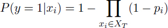
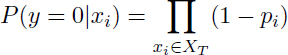

Figure 2.11. Noisy-OR structures
The Noisy-OR (N-OR) structure implies that y = 0 with a probability equal to 1 if all its parent variables xi = 0. However, in many cases this is an unrealistic assumption. It is difficult to capture all the causes of y in several situations (e.g. for reliability to define all the failure modes of a component). Therefore, Henrion [HEN 89] proposed an extension of the N-OR structure called Leaky Noisy-OR (LN-OR) by introducing a new parameter called “leak probability”. The leak probability corresponds to other unknown parents that may affect y. These parents are modeled by using the variable L with a link probability pi = l (Figure 2.12). Let l be the leak probability, such that 0 ≤ l ≤ 1, which is defined as follows:

Figure 2.12. Leaky Noisy-OR structures
Henrion [HEN 89] proposed the following parameterization of the LN-OR structure with n + 1 parameters:


Diez [DIE 93] gave another parameterization of the LN-OR structure as follows:


These two parameterizations are mathematically equivalent, but the difference is related to the question the experts are asked to elicit knowledge. Henrion’s parameterization led to the following question: “What is the probability that y is true given that xi is true and all other modeled variables are false?” Diez’s parameterization is supported by the following question: “What is the probability that y is true given that xi is true and all other modeled and non-modeled variables are false?” In Henrion’s parameterization, experts have to consider a combined influence of xi and the leak on y. In Diez’s parameterization, experts have to consider the link between xi and y with the leak being absent.
The parameters defined earlier can be uncertain too. For example, the influence of a parent variable on a child variable, but also the number of non-modeled parent variables or the state of parent variables cannot be well known. In risk analyses, experts often use intervals to assess different variables. For example, intervals can be used to assess the state of a parent variable or the influence of a parent variable on the child variable. It is, therefore, necessary to take into account uncertainties relating to the link probabilities, the leak probability and the state of parent variables xi. Scientific contributions already exist in relation to the problem of uncertainty in logical structures such as N-OR or LN-OR. Srinivas [SRI 93] and Diez [DIE 93] proposed an extension of the N-OR structure for non-Boolean variables. Antonucci [ANT 11] developed an imprecise LN-OR structure with uncertainty on the link probabilities that can be extended to uncertainty on the leak probability with Diez’s parameterization.
2.5. Industrial applications
Over the past few years, several modeling approaches have dealt with a global view of risks, accounting for technical aspects while being immersed in human, organizational and environmental contexts. [PAT 96] developed the system–action–management (SAM) approach and [SVE 02] highlighted the importance of considering different actors in the risk analysis of an industrial system through a graphical representation of causal flow of accidents (AcciMap). Moreover, [PAP 03] developed the I-Risk method that can account for both technical and organizational characteristics in system risk analysis for the chemical industry. [PLO 04], with MIRIAM1-ATHOS2, evaluated major risk management systems examining technical, human and organizational factors. [CHE 06] focused on the representation of accidental scenarios via the bowtie formalism to facilitate the organizational learning process and [MOH 09] proposed a means of carrying out probabilistic safety studies by taking organizational factors into account.
A recent method was proposed during an academic/industrial collaboration by EDF, INERIS (L’Institut National de l’Environnement Industriel et des Risques) and CRAN (Research Center for Automatic Control of Nancy) [LÉG 09]. This method is called integrated risk analysis. It focuses on a unified risk modeling. The model is multidisciplinary and generic. The generic property comes from a bowtie node for the technical parts, which serves as a basis from which to integrate knowledge about the human, organizational and environmental contexts through the barriers’ efficiency that mitigate the influences of basic events on the consequences of accidental situations.
This modeling methodology has been applied to the assessment of risks in an industrial power plant and, more precisely, to the assessment of technical, human and organizational mitigation actions [LÉG 08a]. The unified model is structured based on the organizational level, the human actions level and their impacts (inhibition) on the propagation of causes and consequences into the bowtie model [LÉG 08a, LÉG 08, LÉG 08b]. The model structure is given in Figure 2.13. The model obtained is used to estimate the occurrence probability of some risk scenarios and to assess the efficiency of barriers on risk reduction. In the risk management process [IEC 09], an engineer can use the model to identify the weaknesses of the socio-technical system and act accordingly to keep the risk criticality below an acceptable level. For the computation part, the model is based on a BN because it combines knowledge and observations to simulate scenarios and to identify weaknesses.
The reader can find an application of this BN-based modeling methodology on a chemical process in [LÉG 09]. In this application, 80 variables are considered. In [DUV 12], a critical system of a power plant is modeled with approximately 110 variables. This latter model is presented in Figure 2.14. The large number of variables in such a model means that only specialists are qualified to understand and perform simulations to characterize risks.

Figure 2.13. Structuration in organizational level and action phases relating to a bowtie model

Figure 2.14. RB unified model of the power plant risk
2.6. Conclusion
This chapter illustrates how BN can solve the modeling problems of dependability and risk analysis of complex systems. This formalism works well with usual Boolean approaches such as FT or RBD. The construction of BN models in such cases follows the same guidelines and gives the same results.
The construction can be automatic by enumerating the cut-sets or tie-sets, whether minimal or not. Moreover, BN is well suited to modeling complex systems where dependencies between variables are not only deterministic.
Several BN structures are feasible for system dependability modeling. Model validation rests on the validation of the method used to build the model and confrontating the model with experiences by testing scenarios to validate the coherence of the model with well-known real cases.
Although BN provides a very compact model of large and complex problems, and makes it possible to handle hundreds of variables, some thousands of variables are needed for large industrial systems. In this case, the BN reach their limits. When the number of variables becomes too large, i.e. if the model cannot be supported in the memory of the computer that handles it, it is then necessary to use a more suitable modeling formalism.