
3
Bayesian Network: Modeling Formalism of the Structure Function of Multi-State Systems
3.1. Introduction
In the case of multi-state systems, standard dependability methods, proposed in the literature are difficult to implement [LIS 03]. In this section, the methodology previously presented in the Boolean case is transposed to multi-state systems to prove that it is easy to obtain multi-state models with BN. Methods are presented for the construction of a model of multi-state systems. The methods are based on cut-sets, tie-sets or the principle of top-down analysis based on functional analysis. Section 3.2.3 explains the functional analysis-based method and explains how it provides an easy way to build an efficient model.
3.2. BN models in the multi-state case
The first step when modeling a multi-state model for dependability analysis is to define the set of variables xi that represent the component states [SHU 10] as follows:

with li being the first failure state, i.e. the component does not satisfy its functioning goals. States 1 … (li – 1) are degraded functioning states, i.e. the component is not fully functional but it does not compromise the system mission. States li … ni are several failure states of the component that can have different consequences on the system state.
The system state is also defined by a multi-state variable with respect to different functioning and malfunctioning scenarios. This variable is denoted as y and takes its values in the following states:

Regarding the complexity of scenarios in a multi-state system, it is difficult or impossible to model the system dysfunction using a FT or the functioning of the system by using a RBD. The analysis based on minimal cut-sets or minimal tie-sets remains efficient, and this method provides the definition of all the scenarios. The BN is an efficient modeling method by which to represent these scenarios. The purpose is to model the state of the system as a function of the components’ states by the multi-state function ϕ. This function can be written as y = ϕ(x), where vector x = (x1, x2, …, xr).
3.2.1. BN model of multi-state systems from tie-sets
The multi-state structure function is easily modeled by a BN. The variables mainly represent the components, the system and the scenarios. The second step is to structure the BN to efficiently link the component variables to the system variable, to encode the functioning and the failure scenarios of the system.
A first solution consists of enumerating all the minimal tie-sets or minimal cut-sets. By applying the same approach as in the binary case, a BN is defined to represent the conditional dependencies linking the system functioning or the failure states of the system with the minimal cut-sets or the minimal tie-sets. For the system shown in Figure 1.2, seven functioning scenarios exist: one is the perfect functioning state and the others are degraded functioning scenarios. In this modeling problem, the degraded states of the system are not modeled; therefore, the system state is defined only by two states: when the system is functioning y = 0; and y = 1 otherwise. The minimal tie-sets are defined from the following combination of components’ states: 0 corresponds to Ok, 1 corresponds to Rc, and 2 corresponds to Ro as defined previously in Table 1.2 of Chapter 1:

Tie-set Lj is said to have occurred (been realized) if the components are in the states that define the tie-set. The occurrence of a tie-set has defined by (Lj = 0). If at least one of the tie-sets is occurred, then the system is in the functioning state y = 0. The BN structure is obtained by linking each of the tie-sets Lj to the variables characterizing the components’ states xi involved in each tie-set (see Figure 3.1).
This approach automatically gives a BN, but the model obtained is not compact and, hence, is difficult to understand. To render the BN more compact, it is pertinent to combine nodes representing minimal tie-sets to the same variables such as {L1, L3}, {L2, L4} and {L5, L6, L7} by creating complex variables and using the full capability of CPT based on multi-state logical combinations.

Figure 3.1. BN structured by the minimal multi-state tie-sets
For {L1, L3}, L13 = L1 ∪ L3 is defined. L13 = 0 for the two scenarios: L1 = {x1 = 0, x2 = 0} and L3 = {x1 = 0, x2 = 2}. In all other cases, L13 = 1 (see Table 3.1). For L24, the CPT is defined in the same manner and is the same as for L13 (see Table 3.2). Finally, for L567, the variable is in state 0 for each scenario: L5 = {x1 = 2, x2 = 0, x3 = 0}, L6 = {x1 = 2, x2 = 1, x3 = 0} and L7 = {x1 = 2, x2 = 0, x3 = 1} (see Table 3.3). This compact BN structure is given in Figure 3.2.

Figure 3.2. Compact BN structured by minimal tie-sets for a multi-state system
Table 3.1. Multi-state L13 tie-set
| x1 | x2 | P(L13 = 0) | P(L13 = 1) |
| 0 | 0 | 1 | 0 |
| 1 | 0 | 1 | |
| 2 | 1 | 0 | |
| 1 | 0 | 0 | 1 |
| 1 | 0 | 1 | |
| 2 | 0 | 1 | |
| 2 | 0 | 0 | 1 |
| 1 | 0 | 1 | |
| 2 | 0 | 1 |
Table 3.2. Multi-state L24 tie-set
| x1 | x3 | P (L24 = 0) | P (L24 = 1) |
| 0 | 0 | 1 | 0 |
| 1 | 0 | 1 | |
| 2 | 1 | 0 | |
| 1 | 0 | 0 | 1 |
| 1 | 0 | 1 | |
| 2 | 0 | 1 | |
| 2 | 0 | 0 | 1 |
| 1 | 0 | 1 | |
| 2 | 0 | 1 |
Table 3.3. Multi-state L567 tie-set
| x1 | x2 | x3 | P(L567 = 0) | P(L567 = 1) |
| 0 | 0 | 0 | 0 | 1 |
| 0 | 1 | 0 | 1 | |
| 0 | 2 | 0 | 1 | |
| 0 | 1 | 0 | 0 | 0 |
| 1 | 1 | 0 | 0 | |
| 1 | 2 | 0 | 0 | |
| 0 | 2 | 0 | 0 | 0 |
| 2 | 1 | 0 | 0 | |
| 2 | 2 | 0 | 0 | |
| 1 | 0 | 0 | 0 | 1 |
| 0 | 1 | 0 | 1 | |
| 0 | 2 | 0 | 1 | |
| 1 | 1 | 0 | 0 | 1 |
| 1 | 1 | 0 | 1 | |
| 1 | 2 | 0 | 1 | |
| 1 | 2 | 0 | 0 | 1 |
| 2 | 1 | 0 | 1 | |
| 2 | 2 | 0 | 1 | |
| 2 | 0 | 0 | 1 | 0 |
| 0 | 1 | 1 | 0 | |
| 0 | 2 | 0 | 1 | |
| 2 | 1 | 0 | 1 | 0 |
| 1 | 1 | 0 | 1 | |
| 1 | 2 | 0 | 1 | |
| 2 | 2 | 0 | 0 | 1 |
| 2 | 1 | 0 | 1 | |
| 2 | 2 | 0 | 1 |
Through the inference mechanism, the probability distribution of y is computed and given by equation [1.3] and the probability distribution of the Li tie-sets are given in Table 3.4.
Table 3.4. Results of the computation based on multi-state and tie-sets
| State | P(y) | P(L13) | P(L24) | P(L567) |
| 0 | 0.345721859 | 0.214953278 | 0.20012291 | 0.066539133 |
| 1 | 0.654278141 | 0.785046723 | 0.79987709 | 0.933460867 |
3.2.2. BN model of multi-state systems from cut-sets
The approach presented in section 3.2.1 can be applied to minimal cut-sets. For the system considered, the following four scenarios can be identified:
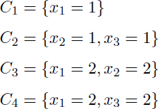

Figure 3.3. BN based on the minimal cut-sets of a multi-state system
The BN model structure is given in Figure 3.3. This structure is different from those built from the minimal tie-sets. This structure is compact and uses multi-states’ modeling ability of BN. The CPT of the minimal C1 to C4 cut-sets are given in Tables 3.5, 3.6, 3.7 and 3.8.
Table 3.5. Multi-state C1 tie-set
| x1 | P(C1 = 0) | P(C1 = 1) |
| 0 | 0 | 1 |
| 1 | 1 | 0 |
| 2 | 0 | 1 |
Table 3.6. Multi-state C2 tie-set
| x2 | x3 | P(C2 = 0) | P(C2 = 1) |
| 0 | 0 | 0 | 1 |
| 1 | 0 | 1 | |
| 2 | 0 | 1 | |
| 1 | 0 | 0 | 1 |
| 1 | 1 | 0 | |
| 2 | 0 | 1 | |
| 2 | 0 | 0 | 1 |
| 1 | 0 | 1 | |
| 2 | 0 | 1 |
Table 3.7. Multi-state C3 tie-set
| x1 | x2 | P(C3 = 0) | P(C3 = 1) |
| 0 | 0 | 0 | 1 |
| 1 | 0 | 1 | |
| 2 | 0 | 1 | |
| 1 | 0 | 0 | 1 |
| 1 | 0 | 1 | |
| 2 | 0 | 1 | |
| 2 | 0 | 0 | 1 |
| 1 | 0 | 1 | |
| 2 | 1 | 0 |
Through the inference mechanism, the probability distributions of any variable can be computed, y, and the minimal C1 to C4 cut-sets are given in Table 3.9. As the model is correct, the probability distribution for y is the same as computed previously (see equation [1.3]).
Table 3.8. Multi-state C4 tie-set
| x1 | x3 | P(C4 = 0) | P(C4 = 1) |
| 0 | 0 | 0 | 1 |
| 1 | 0 | 1 | |
| 2 | 0 | 1 | |
| 1 | 0 | 0 | 1 |
| 1 | 0 | 1 | |
| 2 | 0 | 1 | |
| 2 | 0 | 0 | 1 |
| 1 | 0 | 1 | |
| 2 | 1 | 0 |
Table 3.9. Results of the computation based on multi-state and cut-sets
| State | P(y) | P(C1) | P(C2) | P(C3) | P(C4) |
| 0 | 0.345721859 | 0.77218 | 0.88195459 | 0.780582261 | 0.776463366 |
| 1 | 0.654278141 | 0.22782 | 0.11804541 | 0.219417739 | 0.223536634 |
As shown in previous sections, a BN model can easily be built from the tie-sets or minimal cut-sets for any type of system: simple, complex, binary or multi-state. The models shown in Figures 3.1, 3.2 and 3.3 are equivalent, even if they do not exhibit the same variables. They are equivalent because they model the same joint probability distribution (y, x1, x2, x3) with different factorizations.
As discussed previously, an automatic construction can be realized. Nevertheless, the models obtained are of large dimension and have no explicit structure. This structure of three layers with components, cut-sets or tie-sets and system missions is not of high interpretability, particularly for industrial systems.
3.2.3. BN model of multi-state systems from functional and dysfunctional analysis
A functional/dysfunctional approach can be used to build a BN without enumerating all functional/dysfunctional scenarios. A functional analysis like IDEF0 associated with a dysfunctional analysis, as proposed in [WEB 01, MUL 04, WEB 06, MED 13, MED 15], can serve to build a more readable structure. This approach is also well suited for multi-state systems.
Functional analysis of a system defines a model structure based on the functions achieved by the system. This analysis is interesting because it provides a model structure according to the levels of abstraction describing the functional architecture. Moreover, the system is not limited to the technical system, but can also include human or organizational levels [MED 11].
A function is achieved in a system if its environment provides the necessary input flows: operating conditions, operating supports, energy, orders, etc. Several input flows may contribute to the achievement of a function and the output flows represent the results of the function; thus, the pattern of a generic function is shown in Figure 3.4.

Figure 3.4. Generic definition of a function and its flows
Each part of the BN model corresponds to the functions defined by the functional analysis. Variables in the BN are defined for each input and output of each function. A generic BN pattern is defined in Figure 3.5 to model functions.

Figure 3.5. Generic BN pattern of a function
BN variables are multi-state and each of the conditional probability tables defines the dependency relationships between variables (not necessarily deterministic CPT). HAZOP and FMEA analysis specifies varying states as the failure modes (operating states, degraded states and failure modes), and these states represent the output flows of the function.
Table 3.10. Variables in the IDEF0 model representing the flow F(i)
| Input flows of the functions | Variables | Output flows |
| F (V1, V2, V3) ; F (water to transfer) ; F (control) | L | F (L) |
| F (V1) ; F (water to transfer) ; F (control) | L1 | F (L1) |
| F (L1) ; F (V2) ; F (control) | L2 | F (L2) |
| F (L1) ; F (V3) ; F (control) | L3 | F (L3) |
| F (V1, V2, V3) ; F (water to transfer) ; F (control) | I | F (I) |
| F (V1) ; F (water to transfer) ; F (control) | I1 | F (I1) |
| F (V2) ; F (water to transfer) ; F (control) | I2 | F (I2) |
| F (I2) ; F (V3) ; F (control) | I3 | F (I3) |
The modeling method is applied to the system shown in Figure 1.2. The functional analysis is given in Figures 3.6, 3.7, 3.8 and 3.9. From functional modeling, the variables x1, x2 and x3 are defined to model the flows F (V1), F (V2) and F (V3), representing the states of the components of the system. The variable y is defined to model the flow F (water transferred) and represents the finality of the system (main function). A variable is defined for each function (Table 3.10) that models the output flow depending on the input flows of the functions.

Figure 3.6. Functional model of the system

Figure 3.7. Model of the function (transfer the fluid)

Figure 3.8. Model of the function (circulate the fluid)

Figure 3.9. Model of the function (stop the fluid)

Figure 3.10. BN model mapped from the functional model of the system
The BN structure shown in Figure 3.10 is deduced from the flows defined in the functional analysis. For instance, functional analysis defines “circulate the fluid 2” function (Figure 3.8), and the output flow F (L2) is represented by the variable L2 in the BN (Figure 3.10). Input flows of this function are F (L1) and F (V2) (for simplicity, F (control) is not modeled in this example); therefore, in the BN, the parents of variable L2 are variables L1 and x2 that model the flows F (L1) and F (V2). The BN model is defined by connecting all the variables representing the input and output flows in the functional analysis. The resulting model is different from the models built from minimal cut-sets and minimal tie-sets; this time the model structure is based on a functional analysis of the system.
The inference in the BN model computes the probability y. The results are equal to those computed from the cut-sets, the tie-sets or from the initial joint law. The probabilities of the variables L and I modeling “circulate the fluid” and “stop the fluid” functions of the system, are presented in Table 3.11. The variables L1, L2, L3, I1, I2 and I3 are presented in Tables 3.12 and 3.13.
Table 3.11. Results of the computation based on the IDEF0 model
| State | P(y) | P(L) | P(I) |
| 0 | 0.345721859 | 0.681027695 | 0.664694164 |
| 1 | 0.654278141 | 0.318972305 | 0.335305836 |
Table 3.12. Results of the computation based on the IDEF0 model Li variables
| State | P(L1) | P(L2) | P(L3) |
| 0 | 0.77218 | 0.524348829 | 0.488172196 |
| 1 | 0.22782 | 0.475651171 | 0.511827804 |
Table 3.13. Results of the computation based on the IDEF0 model Ii variables
| State | P(I1) | P(I2) | P(I3) |
| 0 | 0.54437 | 0.51843 | 0.264083058 |
| 1 | 0.45563 | 0.48157 | 0.735916942 |
The proposed approach to building the BN structure of the industrial system is a generalization of the other modeling methods to the multi-state case. This method is suitable for Boolean models as well as multi-state models. The method is based on the hierarchical description of the system functions because the chosen functional analysis provides the hierarchical description of the system functions; nevertheless, this principle may be transposed to other functional analyses to avoid this hypothesis.
3.3. Non-deterministic CPT
For a multi-state system, the relation between the variable y and its parents xi can be non-deterministic, as mentioned in section 2.4. If the conditional probabilities defining y are in the 0, 1 interval then the CPT is deterministic. However, if these conditional probabilities are in the ]0, 1[ interval, then the CPT is non-deterministic. As in the binary case, this kind of CPT means that the expert is not completely sure that the occurrence of xi leads to the occurrence of y. Non-deterministic CPT is encountered for several reasons: the relation between xi and y is naturally non-determinist or some parents (xi) are missing from the model. The inability of an expert to define the relation between xi and y with complete certainty is translated into a non-deterministic CPT.
Let us illustrate this concept using an industrial example. The Omega-20 methodology is dedicated to modeling human safety barrier (HSB) performance. As mentioned in [MIC 09], the assessment of the performance aims to determine the level of confidence in the barrier. The probability of efficiency of the HSB corresponds to a risk reduction factor of the critical event propagation. The HSB is Efficient or Not Efficient; if the HSB is Efficient, the propagation of the critical event is reduced by 100%, and the occurrence of this accident becomes equal to 0; if the HSB is Not Efficient, the critical event propagation is not reduced, and the occurence of the accident is not affected by the HSB.
Moreover, the HSB is based on three steps: detection, diagnosis and action. Each of these steps has a performance classified as follows: 0, 1 or 2. The barrier acts to inhibit the critical event. As shown in Figure 3.11, the HSBs reduce the probability that an event xA propagates its effect to the output y. If the detection is inefficient (confidence level 0), the diagnostic is of low quality and the action has a high stress level, and the event can propagate fully. If all these steps are at their best level, the efficiency probability is equal to 1 and the event xA cannot be propagated. When one of the steps is at level 1, it divides the probability of the critical event propagation by 10, and by 100 at level 2. Then, if detection and diagnostic are at level 1, then the HSB efficiency has a probability equal to 0.01. Therefore, the efficiency probability takes values from 0.000001 to 1, as defined in Table 3.14.

Figure 3.11. BN model of a human safety barrier (HSB)
This methodology is used in the protection and prevention phases in a bowtie model. For instance, it has been used in [LÉG 09, DUV 12] for the integrated risk analysis methodology (Figure 2.14) applied to a chemical process. According to OMEGA20 methodology, it can easily be introduced in many technical systems modeled by a bowtie.
3.4. Industrial applications
The advantages of this modeling approach are particularly interesting when large systems are modeled. This section discusses an application of the modeling method to an industrial case to provide a model for decision-making in maintenance strategy evaluation. The maintenance process is fundamental to improving the availability and productivity of industrial systems. To control these performances, maintenance managers need to be able to choose a maintenance strategy and adequate resources to perform this strategy.
Table 3.14. CPT of HSB efficiency
| Detection | Diagnostic | Action | P(HSB = Efficient) | P(HSB = NotEfficient) |
| 0 | 0 | 0 | 1 | 0 |
| 0 | 0 | 1 | 0.1 | 0.9 |
| 0 | 0 | 2 | 0.01 | 0.99 |
| 0 | 1 | 0 | 0.1 | 0.9 |
| 0 | 1 | 1 | 0.01 | 0.99 |
| 0 | 1 | 2 | 0.001 | 0.999 |
| 0 | 2 | 0 | 0.01 | 0.99 |
| 0 | 2 | 1 | 0.001 | 0.999 |
| 0 | 2 | 2 | 0.0001 | 0.9999 |
| 1 | 0 | 0 | 0.1 | 0.9 |
| 1 | 0 | 1 | 0.01 | 0.99 |
| 1 | 0 | 2 | 0.001 | 0.999 |
| 1 | 1 | 0 | 0.01 | 0.99 |
| 1 | 1 | 1 | 0.001 | 0.999 |
| 1 | 1 | 2 | 0.0001 | 0.9999 |
| 1 | 2 | 0 | 0.001 | 0.999 |
| 1 | 2 | 1 | 0.0001 | 0.9999 |
| 1 | 2 | 2 | 0.00001 | 0.99999 |
| 2 | 0 | 0 | 0.01 | 0.99 |
| 2 | 0 | 1 | 0.001 | 0.999 |
| 2 | 0 | 2 | 0.0001 | 0.9999 |
| 2 | 1 | 0 | 0.001 | 0.999 |
| 2 | 1 | 1 | 0.0001 | 0.9999 |
| 2 | 1 | 2 | 0.00001 | 0.99999 |
| 2 | 2 | 0 | 0.0001 | 0.9999 |
| 2 | 2 | 1 | 0.00001 | 0.99999 |
| 2 | 2 | 2 | 0.000001 | 0.999999 |
A decision-making application in maintenance is proposed by Medina-Oliva [MED 11]. The author formalizes a methodology to develop a model to evaluate and compare different maintenance strategies. The model required merges many complementary views of the system: a functional view of the system, a dysfunctional view of the system, an organization view of the maintenance department and the technical maintenance team, and the effectiveness of its action policy according to the logistics.

Figure 3.12. BN model of the interaction between maintenance and performance of a food system
It is impossible to formalize such a model as a monolithic set of interconnected variables. The model structure is based on fusion of the technical description of the functional view as described in the previous section and the integration of the human and organizational layer presented in Léges et al.’s PhD thesis [LÉG 08a, LÉG 09]. The methodology lies in the unification of different types of knowledge required for the construction of this model [MED 13, MED 15]. In this application, the BN reaches its limit; therefore, a probabilistic relational model (PRM) language is used to define the BN model and a specific inference algorithm is used to compute the probabilities in this very large model.
The model structure is built by the instantiation of several generic and modular patterns. The patterns are dedicated to modeling the decision variables for maintenance and the variables of the industrial system [MED 11]. This method facilitates the structuring and validation of the model.
Medina–Oliva’s PhD these [MED 11, MED 13] describe an application of the method to modeling the interaction between maintenance and performance of a food system. The model is shown in Figure 3.12 (with 700 variables). The computation is only performed on a specific part of the model built partially to answer queries. The global model is never represented entirely by the inference algorithm. This modeling methodology results from the ANR SKOOB [ANR 11] project, and the modeling method is applied in partnership with SOREDAB on the maintenance of a food system [MED 13, MED 15].
3.5. Conclusion
This chapter illustrates how BN can solve the modeling problems of dependability and risk analysis of complex systems. This formalism is well suited to modeling complex multi-state systems where dependencies between variables are not only deterministic. Modeling with BN is an efficient and flexible solution for analysis of simple to complex systems and from binary to multi-state systems.
The modeling methodology based on functional and dysfunctional analysis proposed in this book coupled with a PRM is a very efficient modeling method for large systems, as confirmed by the applications of the ANR SKOOB project [MED 13, MED 15, ANR 11]. Inference algorithms based on PRM are still being developed [SOM 10, KN 10, GON 11]; nevertheless, a PRM modeling platform is provided by Bayesia-BRICKS (Bayesian Representation and Inference for Complex Knowledge Structuring). The PRM provides a framework for knowledge capitalization by creating generic classes and by instantiation of the model to particular systems. This modeling formalism is the future of probabilistic graphical models.
The models presented in this chapter are based on static representations, they do not take into account the temporal dimension. In dependability, it is important to model the temporal dimension to incorporate the impact of the environment, the system operating conditions, the aging and the degradation of components. Such modeling allows evaluation of the behavior of the probabilities of events occurring over time in order to predict future situations. The objective may be, for example, to anticipate the system degradations. This temporal dimension is presented in the next chapter.