
Chapter 5: Online Anomaly Detection
Anomaly detection is a good starting point for machine learning on streaming data. As streaming data delivers a continuous stream of data points, use cases of monitoring live solutions are among the first that come to mind.
There are many domains in which monitoring is essential. In IT solutions, there is generally continuous logging of what happens in the systems, and those logs can be analyzed as streaming data.
In the Internet of Things (IoT), sensor data is being collected on sometimes a large number of sensors. This data is then analyzed and used in real time.
Real-time and online anomaly detection can be of great added value in such use cases by finding values that are far from the expected range of measurements, or otherwise unexpected. Detecting them on time can have great value.
In this chapter, you will first get an in-depth overview of anomaly detection and the theoretical considerations to take into account when implementing it. You will then see how to implement online anomaly detection using the River package in Python.
This chapter covers the following topics:
- Defining anomaly detection
- Use cases of anomaly detection
- Comparing anomaly detection and imbalanced classification
- Algorithms for detecting anomalies in River
- Going further with anomaly detection
Technical requirements
You can find all the code for this book on GitHub at the following link: https://github.com/PacktPublishing/Machine-Learning-for-Streaming-Data-with-Python. If you are not yet familiar with Git and GitHub, the easiest way to download the notebooks and code samples is the following:
- Go to the link of the repository.
- Go to the green Code button.
- Select Download ZIP.
When you download the ZIP file, unzip it in your local environment, and you will be able to access the code through your preferred Python editor.
Python environment
To follow along with this book, you can download the code in the repository and execute it using your preferred Python editor.
If you are not yet familiar with Python environments, I would advise you to check out Anaconda (https://www.anaconda.com/products/individual), which comes with Jupyter Notebooks and JupyterLabs, which are both great for executing notebooks. It also comes with Spyder and VSCode for editing scripts and programs.
If you have difficulty installing Python or the associated programs on your machine, you can check out Google Colab (https://colab.research.google.com/) or Kaggle Notebooks (https://www.kaggle.com/code), which both allow you to run Python code in online notebooks for free, without any setup to do.
Defining anomaly detection
Let's start by creating an understanding of what anomaly detection is. Also called outlier detection, anomaly detection is the process of identifying rare observations in a dataset. Those rare observations are called outliers or anomalies.
The goal of anomaly detection is to build models that can automatically detect outliers using statistical methods and/or machine learning. Such models can use multiple variables to see whether an observation should be considered an outlier or not.
Are outliers a problem?
Outliers occur in many datasets. After all, if you consider a variable that follows a normal distribution, it is normal to see data points far away from the mean. Let's consider a standard normal distribution (a normal distribution with mean 0 and standard deviation 1):
Code Block 5-1
import matplotlib.pyplot as plt
import numpy as np
import scipy.stats as stats
x = np.linspace(-4,4, 100)
plt.plot(x, stats.norm.pdf(x, 0, 1))
You can see the resulting figure as follows:
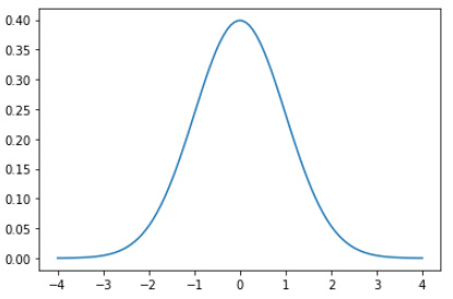
Figure 5.1 – The normal distribution
This standard normal distribution has most of its observations around 0. However, it is normal to observe some observations in the tails of the distribution. If you have a variable that really follows this distribution, and your sample size is big enough, having some observations far away from the center cannot really be considered something bad.
In the following code, you see how a sample of 10 million observations is drawn from a standard normal distribution:
Code Block 5-2
import numpy as np
import matplotlib.pyplot as plt
data = np.random.normal(size=10000000)
plt.hist(data, bins=25)
The data follows the normal curve quite well. You can see this in the following graph:

Figure 5.2 – The normal distribution histogram
Now, let's see what the highest and lowest values of this sample are by using the following code:
Code Block 5-3
min(data), max(data)
In the current draw, a minimum of 5.11 and a maximum of 5.12 were observed. Now, are those outliers or not? The answer is complicated. Of course, the two values are perfectly within the range of the normal distribution. On the other hand, they are extreme values.
This example illustrates that defining an outlier is not always easy, and needs careful consideration for your specific use case. We will now see a number of use cases of anomaly detection.
Exploring use cases of anomaly detection
Before moving on to some specific algorithms for anomaly detection, let's first consider some use cases that are often done with anomaly detection.
Fraud detection in financial institutions
A very common use case for anomaly detection is the detection of fraud in financial institutions. Banks generally have a lot of data, as almost everyone has one or more bank accounts that are used on a regular basis. All these usages generate a huge amount of data that can help banks to improve their services and their profits. Fraud detection is a key component of data science applications in banks, together with many other use cases.
A common use case for fraud detection is to automatically detect credit card fraud. Imagine that your card or card details have been stolen and someone is fraudulently using them. This leads to fraudulent transactions, which could be automatically detected by a machine learning algorithm. The bank could then automatically block your card and ask you to validate whether it was you, or someone fraudulently making these payments.
This is both in the interest of the bank and of the user, so it is a great use case for anomaly detection. Other companies that work with credit card and payment data may also use these methods.
Streaming models are great for fraud detection. There is generally a huge amount of data that comes in in a continuous stream of payments and other data. Streaming models allow you to take action directly when a fraud situation occurs, rather than waiting for the next batch to be launched.
If you want to read more about fraud detection in financial institutions, you can check out the following links:
- https://www.miteksystems.com/blog/how-does-machine-learning-help-with-fraud-detection-in-banks
- https://www.sas.com/en_us/software/detection-investigation-for-banking.html
Anomaly detection on your log data
A second use case for anomaly detection is log analysis. Many software applications generate huge amounts of logs containing all types of information on the execution of programs. These logs are often stored temporarily or long-term for further analysis. In some cases, these analyses may be manual searches of specific information about what happened at some point in software, but at other times they may be automated log treatment programs.
One of the difficulties with anomaly detection in logs is that log data is generally very unstructured. Often, they are just a bunch of printed statements one after the other in a text file. It is very hard to make sense of this data.
If you succeed in the challenge of structuring and categorizing your log data correctly, you can then use machine learning techniques to automatically detect problems with the execution of your software. This allows you to take action straight away.
Using streaming analysis rather than batch analysis is important here as well. Some software is mission-critical, and downtime often means problems for the company. These can be different types of problems, including contractual problems and loss of revenue. If a company can automatically detect bugs, this allows them to move fast and quickly repair the problems. The faster a problem is repaired, the fewer problems for the company.
For deeper use case literature on anomaly detection on log data, you can have a look at the following links:
- https://www.zebrium.com/blog/using-machine-learning-to-detect-anomalies-in-logs
- https://arxiv.org/abs/2202.04301
Fault detection in manufacturing and production lines
An example of fault detection in production lines is the business of industrial food production. Many production lines are almost fully automated, meaning that there is almost no human intervention between the input of raw products and the output of finalized products. The risk of this is that defects might be occurring that cannot be accepted as final products.
The use of sensor data on production lines can strongly help in detecting anomalies in production. When a production line has some parameters that go wrong, sensors, in combination with streaming systems and real-time alerting systems, can allow you to stop the production of faulty products immediately. This can save a lot of money, as producing waste is very costly.
Using streaming and real-time analytics here is also important. The longer you take to respond to a problem, the more waste you produce and the more money is lost. There is a huge return on investment to gain from implementing real-time and streaming analytics systems in manufacturing and production lines.
The following links will allow you to learn more about this use case:
- https://www.scienced irect.com/science/article/pii/S2212827119301908
- https://www.merl.com/publications/docs/TR2018-097.pdf
Hacking detection in computer networks (cyber security)
Automated threat detection for cyber security is another great use case of anomaly detection. Just like the other use cases, positive occurrences are very rare compared to negative cases. The importance of those positive cases, however, is far more impactful than the negative ones.
With recent developments, there is a much higher impact of cyber security problems and leaks for companies than before. Personal data can be sold for a large amount of money and hackers often try to steal this information thinking that they can remain anonymous behind their computers.
Threat and anomaly detection systems are automated systems using machine learning to detect behavior that is not normal and that may represent intrusions. If companies can react quickly to such events happening, they can avoid large public shaming campaigns and potential lawsuits costing lots of money.
Streaming and real-time systems are crucial here as well, as leaving as little time as possible for intruders to act will strongly reduce the risk of any cyber criminality happening in your organization.
The following two articles give a good deep dive into such use cases:
- https://securityboulevard.com/2021/07/what-is-anomaly-detection-in-cybersecurity/
- https://www.xenonstack.com/insights/cyber-network-security
Medical risks in health data
The medical world has seen a large number of inventions over the last years. Part of this is in personal tools such as smart watches and other connected health devices that allow you to measure your own health KPIs in real time. Other use cases can be found in hospitals and other professional health care applications.
When anomalies occur in your health KPIs, it is often of utmost importance to intervene straight away. Health KPI signals can often occur even before we, as humans, start to notice that our health is deteriorating. Even if it is shortly after an event happens, the information will be able to get you the right care without spending much time looking for resources on the causes of your problem.
In general, most of your health metrics will be good, or at least acceptable, until that one metric tells you that something is really going wrong and you need help. In such scenarios, it is important to work with streaming analytics rather than batch analytics. After all, if the data arrives the next hour or the next day, it may well be too late for you. This is another strong argument for using streaming analytics rather than batch analytics.
You can read more about this over here:
Predictive maintenance and sensor data
The last use case that will be discussed here is the use case of predictive maintenance. Many companies have critical systems that need preventive maintenance; if something breaks, this will cost a lot of money or even worse.
An example is the aviation industry. If an airplane crashes, this costs a lot of lives. Of course, no company can predict all anomalies, but any anomaly that could be detected before a crash happens would be a great win.
Anomaly detections can be used for predictive maintenance in many sectors that have comparable problems; if you can predict that your critical system will fail soon, you can have just enough time to do maintenance on the part that needs it and avoid larger problems.
Predictive maintenance can sometimes be done in batch, but it can also benefit from streaming. It all depends on the amount of time you have between detecting an anomaly and the intervention being needed.
If you have a predictive maintenance model that predicts airplane engine failure between now and 30 minutes, you have a large need to get this data to your pilot as soon as possible. If you have predictive systems that tell you that a part needs changing in the coming month, you can probably use batch analytics as well.
To read more about this use case, you can check out the following links:
- https://www.knime.com/blog/anomaly-detection-for-predictive-maintenance-EDA
- https://www.e3s-conferences.org/articles/e3sconf/pdf/2020/30/e3sconf_evf2020_02007.pdf
In the next section, you will see how anomaly detection models compare to imbalanced classification.
Comparing anomaly detection and imbalanced classification
For detecting positive cases against negative cases, the standard go-to family of methods would be classification. For the problems described, as long as you have historical data on at least a few positive and negative cases, you can use classification algorithms. However, you have a very common problem: there are only very few observations that are anomalies. This is a problem that is generally known as the problem of imbalanced data.
The problem of imbalanced data
Imbalanced datasets are datasets in which the target class has very unevenly distributed occurrences. An often-occurring example is website sales: among 1,000 visitors, you often have at least 900 visitors that are just watching and browsing, as opposed to maybe 100 who actually buy something.
Using classification methods carelessly on imbalanced data is prone to errors. Imagine that you fit a classification model that needs to predict for each website visitor whether they will buy something. If you create a very bad model that only predicts non-buying for every visitor, then you will still be right for 900 out of the 1,000 visitors and your accuracy metric will be 90%.
There are a number of standard approaches against this imbalanced data, including using the F1 score and using SMOTE oversampling.
The F1 score
The F1 score is a great replacement for the accuracy score in cases of unbalanced data. Accuracy is computed as the number of correct predictions divided by the total number of predictions made.
This is the formula for accuracy:

The F1 score, however, takes into account the precision and recall of your model. The precision of a model is the percentage of predicted positives that are actually correct. The recall of your model shows the percentage of positives that you were actually able to detect.
This is the formula of precision:

This is the formula of recall:

The F1 score combines those two into one metric, using the following formula:

Using this metric for evaluation, you will avoid interpreting very bad models as good models, especially in the case of imbalanced data.
SMOTE oversampling
SMOTE oversampling is the second method that you can use for counteracting imbalance in your data. It is a method that will create fake data points that strongly resemble the data points in your positive class. By creating a number of data points, your model will be able to learn much better about the positive class, and by using the original positives as the source, you guarantee that the newly generated data points are not too far off.
Anomaly detection versus classification
Although imbalanced classification problems can sometimes work well for anomaly detection problems, there is a reason that anomaly detection is treated as a separate category of machine learning.
The main difference is in the importance of understanding what the positive (anomaly) class looks like. In classification models, you want a model that is easily able to distinguish between two (positives and negatives) or more classes. For this to work, you want your model to learn what each class looks like. The model will search for variables that describe one class, and for other variables or values that describe the other class.
In anomaly detection, you don't really care what the anomaly class looks like. What you need much more, is your model to learn what is normal. As long as your model has a very good understanding of the normal, negative class, it will be able to state normal versus abnormal quite well. This can be an anomaly in any direction and in any sense of the word. It is not needed for the model to have seen such a type of anomaly before, just to know that it is not normal.
In the case of a first anomaly, a standard classification model would not know what this observation should be classified into. If you're lucky, it could go into the anomaly class, but you have no reason to believe it will. However, an anomaly detection model that focuses on what it knows versus what it does not know would be able to detect this anomaly as something that it has not seen before and, therefore, class it as an anomaly.
In the next section, you will see a number of algorithms for anomaly detection that are available in Python's River package.
Algorithms for detecting anomalies in River
In this chapter, you will again use River for online machine learning algorithms. There are other libraries out there, but River is a very promising candidate for being the go-to Python package for online learning (except for reinforcement learning).
You will see two of the online machine learning algorithms for anomaly detection that River currently (version 0.9.0) contains, as follows:
- OneClassSVM: An online adaptation of the offline version of One-Class SVM
- HalfSpaceTrees: An online adaptation of Isolation Forests
You will also see how to work with the constant thresholder and the quantile thresholder.
The use of thresholders in River anomaly detection
Let's first look at the use of thresholders, as they will be wrapped around the actual anomaly detection algorithms.
Anomaly detection algorithms will generally return a score between 0 and 1 to indicate to the model to what extent the observation is an anomaly. Scores closer to 1 are more likely to be an outlier, and scores closer to 0 are considered more normal.
In practice, you need to decide on a threshold to state for each observation whether you expect it to be an outlier. To convert the continuous 0 to 1 scale into a yes/no answer, you use a thresholder.
Constant thresholder
The constant thresholder is the simplest approach that you would intuitively come up with. You will give a constant value that will split observations with a continuous (0 to 1) anomaly score into yes/no anomalies based on being higher or lower than the constant.
As an example, if you specify a value of 0.95 to be your constant threshold, every observation with an anomaly higher than that will be considered an anomaly, and every data point that is scored lower than that is not considered an anomaly.
Quantile thresholder
The quantile thresholder is slightly more advanced. Rather than a constant, you specify a quantile. You have seen quantiles before in the chapter on descriptive statistics. A 0.95 quantile means that 95% of the observations are below this value and 5% of the observations are above it.
Imagine that you used a constant threshold of 0.95, but the model has detected no points above 0.95. In this case, the constant thresholder would split no observations at all into the anomaly class. The quantile thresholder of 0.95 would still give you exactly 5% of your observations as anomalies.
The preferred behavior will depend on your use case, but at least you have the two options at the ready for your anomaly detection in River.
Anomaly detection algorithm 1 – One-Class SVM
Let's now move on to the first anomaly detection algorithm: One-Class SVM. You'll first see a general overview of how One-Class SVM works for anomaly detection. After that, you'll see how it is adapted for an online context in River and you'll do a Python use case using One-Class SVM in Python.
General use of One-Class SVM on anomaly detection
One-Class SVM is an unsupervised outlier detection algorithm based on the Support Vector Machine (SVM) classification algorithm.
SVMs are commonly used models for classification or other supervised learning. In supervised learning, they are known to be great for using the kernel trick, which maps the inputs into high-dimensional feature spaces. With this process, SVMs are able to generate non-linear classification.
As described earlier, anomaly detection algorithms need to understand what is normal, but they don't have to understand the non-normal classes. The One-Class SVM is, therefore, an adaptation of the regular SVMs. In regular, supervised SVMs, you need to specify the classes (target variable), but in One-Class SVM, you act like all the data is in a single class.
Basically, the One-Class SVM will just fit an SVM in which it tries to fit a model that best predicts all of the variables as the same target class. When the model fits well, the maximum of individuals will have a low error in their prediction.
Individuals with a high error score for the best-fitting model are difficult to predict using the same model as for the other individuals. You could consider that they may need another model and, therefore, hypothesize that the individuals do not come from the same data-generating process. They may well, therefore, be anomalies.
The error is used as a thresholding score to split individuals. Individuals with a high error score can be classified as anomalies and individuals with a low error score can be considered normal. This split is generally done with a quantile threshold, which was introduced earlier.
Online One-Class SVM in River
The OneClassSVM model in River is described in the documentation as a stochastic implementation of the One-Class SVM and it will not, unfortunately, perfectly match the offline definition of the algorithm. If it is important for your use case to find exact results, you could try out online and offline implementations and see how much they differ.
In general, outlier detection is an unsupervised task, and it is hard to be totally sure about the final answer and precision of your models. This is not a problem as long as you monitor results and take KPI selection and tracking of your business results seriously.
Application on a use case
Let's now apply the online training process of a One-Class SVM using River.
For this example, let's create our own dataset so that we can be sure of the data that should be considered an outlier or not:
- Let's create a uniform distribution variable with 1,000 observations between 0 and 1:
Code Block 5-4
import numpy as np
normal_data = np.random.rand(1000)
- The histogram of the current run can be prepared as follows, but it will change due to randomness:
Code Block 5-5
import matplotlib.pyplot as plt
plt.hist(normal_data)
The resulting plot will show the following histogram:

Figure 5.3 – Plot of the normal data
- As we know this distribution very well, we know what to expect: any data point between 0 and 1 is normal and every data point outside 0 to 1 is an outlier. Let's now add 1% of outliers to the data. Let's make 0.5% of easy-to-detect outliers (random int between 2 and 3 and between -1 and -2), which is very far away from our normal distribution. Let's also make 0.5% of our outliers a bit harder to detect (between 0 and -1 and between 1 and 2).
This way we can challenge the model and see how well it performs:
Code Block 5-6
hard_to_detect = list(np.random.uniform(1,2,size=int(0.005*1000))) +
list(np.random.uniform(0,-1,size=int(0.005*1000)))
easy_to_detect = list(np.random.uniform(2,3,size=int(0.005*1000))) +
list(np.random.uniform(-1,-2,size=int(0.005*1000)))
- Let's put all that data together and write code to deliver it to the model in a streaming fashion, as follows:
Code Block 5-7
total_data = list(normal_data) + hard_to_detect + easy_to_detect
import random
random.shuffle(total_data)
for datapoint in total_data:
pass
- Now, the only thing remaining to do is to add the model into the loop:
Code Block 5-8
# Anomaly percentage for the quantile thresholder
expected_percentage_anomaly = 20/1020
expected_percentage_normal = 1 - expected_percentage_anomaly
Code Block 5-9
!pip install river
from river import anomaly
model = anomaly.QuantileThresholder(
anomaly.OneClassSVM(),
q=expected_percentage_normal
)
for datapoint in total_data:
model = model.learn_one({'x': datapoint})
When running this code, you have now trained an online One-Class SVM on our synthetic data points!
- Let's try to get an idea of how well it worked. In this following code, you see how to obtain the scores of each individual and the assignment to the classes:
Code Block 5-10
scores = []
for datapoint in total_data:
scores.append(model.score_one({'x': datapoint}))
- As we know the actual result, we can now compare whether the answers were right. You can use the following code for that:
Code Block 5-11
import pandas as pd
results = pd.DataFrame({'data': total_data , 'score': scores})
results['actual_outlier'] = (results['data'] > 1 ) | (results ['data'] < 0)
# there are 20 actual outliers
results['actual_outlier'].value_counts()
The results are shown here:

Figure 5.4 – The results of Code Block 5-11
Code Block 5-12
# the algo detected 22 outliers
results['score'].value_counts()
The following figure shows that 22 outliers were detected:

Figure 5.5 – The results of Code Block 5-12
- We should now compute how many of the detected outliers are actual outliers and how many are not actual outliers. This is done in the following code block:
Code Block 5-13
# in the 22 detected otuliuers, 10 are actual outliers, but 12 are not actually outliers
results.groupby('actual_outlier')['score'].sum()
The result is that out of the 22 detected outliers, 10 are actual outliers, but 12 are not actually outliers. This can be seen in the following figure:

Figure 5.6 – The results of Code Block 5-13
The obtained result is not too bad: at least some of the outliers were detected correctly, and this could be a good minimum viable product to start automating anomaly detection for this particular use case. Let's see whether we can beat it with a different anomaly detection algorithm!
Anomaly detection algorithm 2 – Half-Space-Trees
The second main anomaly detection algorithm that you'll see here is the online alternative to Isolation Forests, a commonly used and performant outlier detection algorithm.
General use of Isolation Forests in anomaly detection
Isolation Forests work a bit differently than most anomaly detection algorithms. As described throughout this chapter, many models do anomaly detection by first understanding the normal data points and then deciding whether a data point is relatively similar to the other normal points or not. If not, it is considered an outlier.
Isolation Forests are a great invention, as they work the other way around. They try to model everything that is not normal, and they try to isolate those points from the rest.
In order to isolate observations, the Isolation Forest will randomly select features and then split the feature between the minimum and the maximum. The number of splits required to isolate a sample is considered a good description of the isolation score of an observation.
If it is easy to isolate it (short path to isolation, equivalent to having little splits to isolate the point), then it is probably a relatively isolated data point, and we could class it as an outlier.
How does it change with River?
In River, the model has to train online, and they had to make some adaptations to make it work. The fact that some adaptations have been made is the reason for callling the model HalfSpaceTrees in River.
As something to keep in mind, the anomalies have to be spread out in the dataset in order for the model to work well. Also, the model needs all values to be between 0 and 1.
Application of Half-Space-Trees on an anomaly detection use case
We will implement this as follows:
- Let's now apply Half-Space-Trees to the same, univariate use case and see what happens:
Code Block 5-14
from river import anomaly
model2 = anomaly.QuantileThresholder(
anomaly.HalfSpaceTrees(),
q=expected_percentage_normal
)
for datapoint in total_data:
model2 = model2.learn_one({'x': datapoint})
scores2 = []
for datapoint in total_data:
scores2.append(model2.score_one({'x': datapoint}))
import pandas as pd
results2 = pd.DataFrame({'data': total_data, 'score': scores2})
results2['actual_outlier'] = (results2 ['data'] > 1 ) | (results2['data'] < 0)
# there are 20 actual outliers
results2['actual_outlier'].value_counts()
The results of this code block can be seen in the following figure. It appears that there are 20 actual outliers:

Figure 5.7 – The results of Code Block 5-14
- You can now compute how many outliers the model detected using the following code:
Code Block 5-15
# the algo detected 29 outliers
results2['score'].value_counts()
It appears that the algorithm detected 29 outliers. This can be seen in the following figure:

Figure 5.8 – The results of Code Block 5-15
- We will now compute how many of those 29 detected outliers were actually outliers to see whether our model is any good:
Code Block 5-16
# the 29 detected outliers are not actually outliers
results2.groupby('actual_outlier')['score'].sum()
The results show that our 29 detected outliers were not really outliers, indicating that this model is not a good choice for this task. There is really no problem with that. After all, this is the exact reason to do model benchmarking:

Figure 5.9 – The results of Code Block 5-16
As you can see, this model is less performant in the current use case. In conclusion, the One-Class SVM performed better at identifying anomalies in our sample of 1,000 draws of a uniform distribution on the interval 0 to 1.
Going further with anomaly detection
To go further with anomaly detection use cases, you can try out using different datasets or even a dataset of your own use case. As you have seen in the example, data points are inputted as a dictionary. In the current example, you used univariate data points: only one entry in the dictionary.
In practice, you generally have multivariate problems, and you would have multiple variables in your input. Models may be able to fit better in such use cases.
Summary
In this chapter, you have learned how anomaly detection works, both in streaming and non-streaming contexts. This category of machine learning models takes a number of variables about a situation and uses this information to detect whether specific data points or observations are likely to be different from the others.
You have gotten an overview of different use cases for this. Some of those are the monitoring of IT systems, or production line sensor data in manufacturing. Whenever it is problematic to have a data point that is too different from the others, anomaly detection is of great added value.
You have finished the chapter by implementing a model benchmark in which you have benchmarked two online anomaly detection models from the River library. You have seen one model being able to detect a part of the anomalies, and the other model having much worse performances. This has introduced you not only to anomaly detection but also to model benchmarking and model evaluation.
In the next chapter, you will see even more on those topics. You will be working on online classification models, and you will again see how to implement model benchmarking and metrics, but this time, for classification rather than anomaly detection. As you have seen in this chapter, classification can sometimes be used for anomaly detection as well, making the two use cases related to each other.
Further reading
- Anomaly Detection: https://en.wikipedia.org/wiki/Anomaly_detection
- River ML Constant Thresholder: https://riverml.xyz/latest/api/anomaly/ConstantThresholder/
- River ML Quantile Thresholder: https://riverml.xyz/latest/api/anomaly/QuantileThresholder/
- Support Vector Machine: https://en.wikipedia.org/wiki/Support-vector_machine
- Scikit Learn One Class SVM: https://scikit-learn.org/stable/modules/generated/sklearn.svm.OneClassSVM.html
- River ML One Class SVM: https://riverml.xyz/latest/api/anomaly/OneClassSVM/
- Isolation Forest: https://en.wikipedia.org/wiki/Isolation_forest
- River ML Half-Space Trees: https://riverml.xyz/latest/api/anomaly/HalfSpaceTrees/