
Chapter 10: Comet for Deep Learning
Deep learning is a subfield of artificial intelligence that aims to extract knowledge from data through complex neural networks. You can imagine a neural network as a collection of nodes (or neurons), which are organized in different layers of processing. Similar to the human brain, which learns in incremental steps, in a neural network, the level of knowledge increases as you move from one layer to the next.
Compared to traditional machine learning algorithms, deep learning algorithms can automatically extract features from incoming data. Therefore, they are able to process even thousands of input features, which is unthinkable for a machine learning algorithm in which you should select the input features by hand.
Running deep learning algorithms is both computationally expensive and resource-consuming. However, over the last few years, their uptake has increased considerably thanks to the development of even more powerful machines as well as the spread of distributed systems for parallel calculations. Today, deep learning finds its major applications in the fields of image and speech recognition. In this chapter, you will review some basic concepts behind deep learning as well as the main types of deep learning networks.
In recent years, different open source tools and libraries have been implemented to perform deep learning, including TensorFlow, Keras, Caffe, PyTorch, and so on. In this chapter, you will review the TensorFlow library and how to integrate it with Comet.
In the last part of this chapter, you will implement a practical use case, which uses the TensorFlow library and tracks the result in Comet.
The chapter is organized as follows:
- Introducing basic deep learning concepts
- Exploring the TensorFlow package
- Using deep learning - from project setup to report building
Before we start to review basic deep learning concepts, let’s install the required software needed to run the examples described in this chapter.
Technical requirements
We will run all of the experiments and code in this chapter using Python 3.8. You can download it from the official website at https://www.python.org/downloads/, choosing the 3.8 version.
The examples described in this chapter use the following Python packages:
- comet-ml 3.23.0
- gradio 3.2.2
- matplotlib 3.2.2
- numpy 1.21.6
- pandas 1.3.4
- tensorflow 2.8.2
We have already described the comet-ml, matplotlib, numpy, and pandas packages and how to install them in Chapter 1, An Overview of Comet. So, please refer back to that for further details on installation.
In this section, you will see how to install the other required packages.
gradio
gradio is a Python package that permits you to build fast demo apps that are fully integrated with your notebooks. You can install gradio as follows:
pip install gradio
For more details on gradio, you can read its official documentation, available at the following link: https://gradio.app/.
tensorFlow
tensorFlow is one of the most popular Python packages for deep learning. You can install it as follows:
pip install tensorflow
You can read more details about TensorFlow in its official documentation, available at the following link: https://www.tensorflow.org/.
Now that you have installed all of the software needed in this chapter, let’s move on to how to use Comet for deep learning, starting with reviewing some basic concepts.
Introducing basic deep learning concepts
The following figure shows how deep learning fits into the field of artificial intelligence:

Figure 10.1 – How deep learning is related to other artificial intelligence fields
You can see that deep learning is a subfield of neural networks, which are a subfield of machine learning, which is a subfield of artificial intelligence. In this section, you will understand the difference between deep learning and neural networks as well as how you can classify deep learning networks.
You will learn some general concepts about deep learning. For more details, you can refer to the books contained in the Further reading section of this chapter.
The section is organized as follows:
- Introducing neural networks
- Exploring the difference between deep learning and neural networks
- Classifying deep learning networks
Let’s start from the first point: introducing neural networks.
Introducing neural networks
The basic building block of a neural network is called a neuron. The objective of a neuron is to represent the behavior of a neuron in our brain through a mathematical model. The simplest neural network is called perceptron, and it is composed of N input features, one single neuron, and one output, as shown in the following figure:

Figure 10.2 – A perceptron
The single neuron is composed of the following two main components:
- The summation, which calculates the summation of the product between the input features and the weights as shown in the following equation:

Weights establish how much each input feature influences the output. Usually, the preceding formula should be corrected by introducing a new term called bias, as shown in the following formula:

- The activation function, which is a nonlinear function, calculates the final output. Common activation functions are the sigmoid function, the hyperbolic tangent, and the rectified linear unit (ReLU).
This process, from input to output, is called forward propagation.
The objective of the learning algorithm for a neural network is to find the best values of weights and bias, which minimize a loss function. This process, which is also known as backward propagation, is achieved through an iterative process that computes the loss function and updates weights and bias at every iteration. As a loss function, usually, you can use mean squared error (MSE) for regression tasks and cross-entropy for classification tasks.
A perceptron is only the basic building block of a neural network. You can build more complex neural networks by adding many neurons and layers. For more details on neural networks, you can read the books listed in the Further reading section.
Now that you have learned the basic concepts behind neural networks, we can move on to the next point: exploring the difference between deep learning and neural networks.
Exploring the difference between deep learning and neural networks
A typical neural network is composed of an input layer, a single hidden layer, and an output layer. Each layer can have a variable number of nodes or neurons. The following figure shows an example of a neural network:

Figure 10.3 – A simple neural network
The neural network of the preceding figure is composed of the following three layers:
- The first layer (input layer) has three nodes.
- The second layer (hidden layers) has four nodes.
- The third layer (output layer) has two nodes.
It is worth noting that nodes in the same layer are not connected directly.
Deep learning is the name used to indicate a neural network that is composed of more than three layers, including the input and the output layers. The following figure shows an example of a deep learning network:

Figure 10.4 – A deep learning network
The preceding figure shows a deep learning network with three hidden layers.
In a deep learning network, each layer receives as input the set of features produced as output by the previous layer. Thus, the deeper the network, the more complex the features the layers can recognize. This is known as feature hierarchy. Thanks to feature hierarchy, deep learning networks can work with very large and high-dimensional data with a huge number of parameters that are learned automatically without human intervention. The output of a deep learning network is a classifier, which assigns a probability to a particular class or label. Deep learning is quite resource-consuming because it requires high-performance GPUs and large amounts of storage to train models.
Now that you have learned the difference between deep learning and neural networks, we can move on to the next point: classifying deep learning networks.
Classifying deep learning networks
You can classify deep learning networks into the following three main categories:
- Artificial neural networks (ANN)
- Recurrent neural networks (RNN)
- Convolutional neural networks (CNN)
Let’s investigate each category separately, starting with the first: artificial neural networks.
Artificial neural networks
An artificial neural network (ANN), also known as a feedforward neural network, is the simplest type of neural network with many neurons in each layer. An ANN processes inputs only in the forward direction, as shown in Figure 10.3.
An ANN has no memory because information moves only in one direction: from the input to the output. This means that an ANN is not able to remember what happened in the past. An ANN makes a decision only based on the current input.
Typically, you use ANNs to solve problems related to tabular data, images, and texts.
Recurrent neural networks
A recurrent neural network (RNN) is a type of neural network that makes decisions based on the current input as well as the inputs received previously. This is achieved by adding a recurrent connection to the hidden layers, as shown in the following figure:

Figure 10.5 – A recurrent neural network
In the preceding figure, the neurons in the hidden layer contain a recurrent connection, which permits the neurons to remember past inputs. In other words, RNNs are networks with memory. Typically, you use RNNs to solve problems related to time series, texts, and audio.
Convolutional neural networks
A convolutional neural network (CNN) is the most popular type of deep learning network, and it is especially used for image recognition and classification, object detection, and recognition of faces. The following figure shows an example of a CNN:

Figure 10.6 – A convolutional neural network
The first two layers, which are called convolutional layer and pooling layer, respectively, are devoted to feature extraction. The convolutional layer is the core of a CNN because it extracts the features from the input. The pooling layer aims at reducing the number of extracted features. The extracted features constitute the input of a fully connected neural network, which calculates the output probability for a given task.
Now that you have reviewed the main types of deep learning networks, we can move on to the next topic: exploring the TensorFlow package.
Exploring the TensorFlow package
TensorFlow is an open source library for deep learning released by the Google Brain team. It supports different programming languages, including Python and Javascript. You can use TensorFlow for different purposes, especially for audio and image analysis. In this chapter, we will focus on TensorFlow 2.x. Since training a model in TensorFlow could be time and resource-consuming, TensorFlow also provides many pre-trained models, stored in the TensorFlow Hub, available at the following link: https://www.tensorflow.org/hub.
Running TensorFlow on your local machine could be computationally expensive and resource-consuming, thus you use Google Colab, a collaborative framework provided by Google, to train your models. In fact, Google Colab provides you with free access to GPU and powerful machines. Google Colab is a valid alternative to Jupyter Notebook and is compatible with it. You can run your first Google Colab notebook at the following link: https://colab.research.google.com/. You can use it as you usually do with Jupyter Notebook.
In this section, we will cover the following aspects:
- Introducing the TensorFlow package
- Integrating TensorFlow with Comet
Let’s start from the first point: introducing the TensorFlow package.
Introducing the TensorFlow package
The following figure shows the main tasks and the related sub-packages provided by the core TensorFlow library:
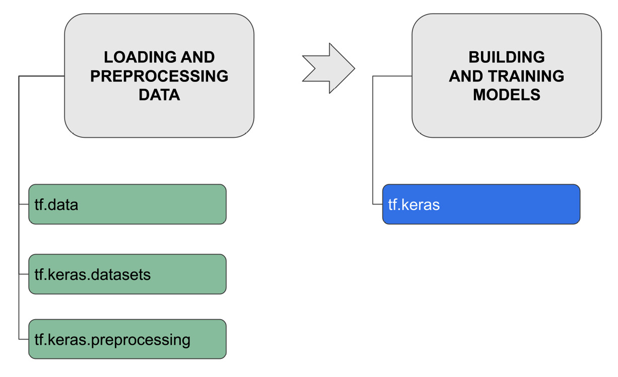
Figure 10.7 – The main tasks in TensorFlow
There are two main tasks as follows:
- Loading and preprocessing data
- Building and training models
The full list of implemented tasks is available in the TensorFlow official documentation, which is available at the following link: https://www.tensorflow.org/api_docs/python/tf.
TensorFlow includes many additional extensions that permit you, for example, to preprocess text, optimize models, and so on. You can find the list of all of the extensions at the following link: https://www.tensorflow.org/resources/libraries-extensions.
Let’s investigate the two described tasks separately, starting with the first one: loading and preprocessing data.
Loading and preprocessing data
To work with TensorFlow, you need to load your dataset as an object belonging to the tf.data.Dataset class. You can do it by hand or by using the API provided by the tf.keras sub-package. To get familiar with TensorFlow datasets, you can use the toy datasets provided by the tf.keras.datasets module, which are ready for use. In addition, you can use the public TensorFlow datasets provided by the TensorFlow extension library, available at the following link: https://github.com/tensorflow/datasets.
In this section, we will explore two simple ways to load your datasets from CSV or images.
Loading a TensorFlow dataset from CSV
The following steps will load a TensorFlow dataset from CSV:
- First, you load the dataset as a pandas DataFrame as follows:
import pandas as pd
dataset_path = 'path/to/csv/file'
df = pd.read_csv(dataset_path)
- Then, you convert it into a dictionary as follows:
dict_df = dict(df)
- Finally, you load the dictionary as a TensorFlow dataset as follows:
import tensorflow as tf
data = tf.data.Dataset.from_tensor_slices(dict_df)
Now you can review how to build a TensorFlow dataset from a set of images.
Loading a TensorFlow dataset from a set of images
Next, let’s try images with the following steps:
- First, you need to organize your set of images. To do so, you need to create a folder for each class label, and each folder must contain the images associated with that class, as shown in the following figure:

Figure 10.8 – An example of the structure of an images folder
In the preceding figure, there are two directories, cat and dog, which correspond to two classes. Each directory contains three images.
- Then, you can extract the training set from your images, as shown in the following code:
train_ds = tf.keras.utils.image_dataset_from_directory(
data_dir,
validation_split=0.2,
subset="training",
seed=123,
image_size=(img_height, img_width),
batch_size=batch_size)
The data_dir parameter specifies the directory where the images are located.
- You can then extract the validation set as follows:
validation_ds = tf.keras.utils.image_dataset_from_directory(
data_dir,
validation_split=0.2,
subset="validation",
seed=123,
image_size=(img_height, img_width),
batch_size=batch_size)
Before using your dataset as an input to a TensorFlow model, you can preprocess it. The tf.keras.preprocessing module provides many functions to preprocess images, texts, and sequence data. For further details, you can refer to the TensorFlow official documentation, available at the following link: https://www.tensorflow.org/api_docs/python/tf/keras/preprocessing.
Now that you have learned how to load and preprocess a dataset in TensorFlow, we can move on to the next point: building and training models.
Building and training models
The simplest way to build a TensorFlow model is to use the classes and functions provided by the tf.keras package as follows:
- First, you define the model as follows:
from tensorflow import keras
model = keras.models.Sequential([
tf.keras.layers.Conv2D(),
tf.keras.layers.MaxPooling2D(),
tf.keras.layers.Flatten(),
tf.keras.layers.Dense(),
])
The preceding example implements a Sequential model, which is a network where each layer has one input tensor and one output tensor. Within the Sequential model, you should specify the list of layers. In the preceding example, the first layer is a convolutional layer for 2D spatial data (Conv2D), followed by a pooling layer for 2D spatial data (MaxPooling2D). Then, there is a flatten (Flatten) layer, and finally, a dense layer (Dense). For simplicity, the preceding code does not show the configuration parameters for each layer. You can read the TensorFlow official documentation at tensorflow.org to learn how to configure the parameters of each layer.
- Then, you compile the model as follows:
model.compile(
optimizer='adam',
loss='sparse_categorical_crossentropy',
metrics=['accuracy']
)
The compile() method receives as input optimizer, the loss function, and the list of metrics to evaluate during the training process.
- Finally, you train the model as follows:
model.fit(
train_features,
train_labels,
validation_data=(test_features, test_labels),
)
The fit() method receives as input the training set and the validation set. In addition, you can specify other parameters, including the number of batches and epochs. You can read the TensorFlow official documentation at tensorflow.org for further details.
Now that you have learned how to build and train a model in TensorFlow, let’s move on to the next point: integrating TensorFlow with Comet.
Integrating TensorFlow with Comet
To make Comet log your TensorFlow models, you need to import the comet_ml library before TensorFlow, as shown in the following piece of code:
from comet_ml import Experiment
import tensorflow as tf
Note
You should always import the comet_ml library before any machine learning library.
If you are using a Keras model included in the TensorFlow library, Comet will automatically log most of the metrics and parameters. In addition, you can configure some specific configuration parameters to log histograms, graphs, hyperparameters, and so on. You can find the list of configuration parameters in the Comet documentation, available at the following link: https://www.comet.ml/docs/v2/integrations/ml-frameworks/keras/.
You can configure the configuration parameters in the following three different (alternative) ways:
- By adding a new line for each configuration parameter in the .comet.config file, as shown in the following piece of code:
[comet]
api_key=YOUR_COMET_API_KEY
workspace=YOUR_WORKSPACE
project_name=YOUR_PROJECT_NAME
[comet_auto_log]
histogram_weights=True
histogram_gradients=True
histogram_activations=True
In the preceding example, in addition to the classical [comet] section, we have added the [comet_auto_log] section and specified that we want to plot histograms related to weights, gradients, and activations.
- By passing the configuration parameters as input to the Experiment class, as shown in the following piece of code:
experiment = Experiment(auto_histogram_weight_logging=True,auto_histogram_gradient_logging=True,auto_histogram_activation_logging=True)
Similar to the case in the earlier example, we have specified that we want to plot histograms related to weights, gradients, and activations.
- By using environment variables, as shown in the following piece of code:
export COMET_AUTO_LOG_HISTOGRAM_WEIGHTS=True
export COMET_AUTO_LOG_HISTOGRAM_ACTIVATIONS=True
export COMET_AUTO_LOG_HISTOGRAM_ACTIVATIONS=True
Also, in this case, we have specified to plot histograms related to weights, gradients, and activations. In Python, we can also set the environment variables directly in our script, as shown in the following piece of code:
import os
os.environ['COMET_AUTO_LOG_HISTOGRAM_WEIGHTS'] = True
We have set the environ variable provided by the os library.
Now that you have learned how to integrate Comet with TensorFlow, we can move on to the final topic: using deep learning- from project setup to report building.
Using deep learning- from project setup to report building
In this section, you will implement a practical example that performs an image classification task. The objective of this example is to build a TensorFlow model that predicts the type of dress represented in an image. The model is fitted with some images representing clothes, and then it is used to predict the type of dress. You will track the model in Comet, and you will build a simple demo interface using Gradio to test the model performance interactively.
The full code of the example described in this section is available at the following link: https://github.com/PacktPublishing/Comet-for-Data-Science/tree/main/10.
You will focus on the following aspects:
- Introducing Gradio
- Loading the dataset
- Implementing a basic model
- Exploring results in Comet
- Building a prediction interface
- Building the final report
Let’s start from the first point: introducing Gradio.
Introducing Gradio
Gradio is a Python library that permits you to build demos and quick web interfaces for testing purposes. Conceptually, a Gradio interface is composed of the following three components:
- Input, which can be either a single element or a list of elements, including textboxes, checkboxes, radio buttons, and many more.
- Function, which is a Python function that receives the input component as input, performs some computation, and returns the output.
- Output, which can be either a single element or a list of elements, including labels, images, plots, and many more.
For more details on the Gradio library, you can read its official documentation, available at the following link: https://gradio.app/docs/. You will see a practical example on how to use Gradio and combine it with Comet in the following sections.
Now that you have learned some basic concepts of Gradio, we can move on to the next step: loading the dataset.
Loading the dataset
As a use case, you will use the Fashion-MNIST set released by Zalando Research and available on GitHub at https://github.com/zalandoresearch/fashion-mnist, released under the MIT license. The dataset contains a training set of 60,000 examples and a test set of 10,000 examples. Each example consists of a 28x28 grayscale image associated with a label from one of the following 10 classes:

Figure 10.9 – The mapping between label and class in the Fashion-MNIST dataset
You can load the dataset through TensorFlow as follows:
- First, we set all of the environment variables as follows:
import os
os.environ['COMET_KERAS_HISTOGRAM_ACTIVATION_INDEX_LIST'] = "1,2"
The preceding variable indicates that we want to build the activation histograms for layers 1 and 2.
- Then, we import all of the required libraries as follows:
from comet_ml import Experiment
import tensorflow as tf
from tensorflow import keras
Note
To make Comet log a TensorFlow model, you should import the comet_ml library before the tensorflow one.
- Then, we use the load_data() method to load the dataset directly from keras as follows:
fashion_mnist = keras.datasets.fashion_mnist
(train_images, train_labels), (test_images, test_labels) =
fashion_mnist.load_data()
We use the keras.dataset.fashion_mnist object provided by keras, and then the load_data() method to retrieve both the training and test sets.
- We can plot the first 25 examples extracted from the training set, as shown in the following piece of code:
n_row = 5
n_col = 5
_, axs = plt.subplots(n_row, n_col, figsize=(12, 12))
axs = axs.flatten()
for img, ax in zip(train_images, axs):
ax.imshow(img)
ax.axis('off')
plt.show()
We have defined a grid of size 5x5, and then we have plotted an image in each cell of the grid through the imshow() method. We have also hidden both axes through the ax.axis('off') statement. The following figure shows the first 25 examples extracted from the training set:

Figure 10.10 – The first 25 examples extracted from the training set
To the human eye, it is quite easy to recognize the class to which each image belongs.
Now that you have loaded the dataset, we can move on to the next step: implementing a simple model.
Implementing a basic model
It is time to build the model with the following steps:
- Since TensorFlow is automatically integrated with Comet, we will first create a Comet experiment where we specify the additional parameters to also log histograms as follows:
experiment = Experiment(auto_histogram_weight_logging=True,auto_histogram_gradient_logging=True,auto_histogram_activation_logging=True)
You need to configure the .comet.config file as explained in Chapter 1, An Overview of Comet. Alternatively, to pass the additional parameters to the Comet experiment, you can include them in the .comet.config file.
- Now, we implement a Sequential model, which is the simplest available model. A Sequential model contains exactly one input tensor and one output tensor for each layer. In our case, we implement a Sequential model with three layers as follows:
model = keras.models.Sequential([
keras.layers.Flatten(input_shape=(28, 28)),
keras.layers.Dense(32, activation='relu'),
keras.layers.Dense(10, activation='softmax')
])
The first layer is a Flatten layer, which receives the image as input. The second layer is a Dense layer with 32 units and a relu activation function. The third layer contains 10 units and a softmax activation function.
- Once you have created the model, we need to compile it by defining the loss function, the optimizer, and the metrics as follows:
model.compile(
optimizer='adam',
loss='sparse_categorical_crossentropy',
metrics=['accuracy']
)
In our case, we have set the optimizer to adam, the loss function to sparse_categorical_cross_entropy, and the list of metrics to accuracy.
- The model is ready to be fitted as follows:
model.fit(
train_images,
train_labels,
epochs=8,
validation_data=(test_images, test_labels),
)
We use the fit() method, which receives as input the training images and their associated labels as well as the number of epochs and data used for validation.
- After fitting, we can plot a model summary as follows:
print(model.summary())
The summary() method returns the output shown in the following figure:
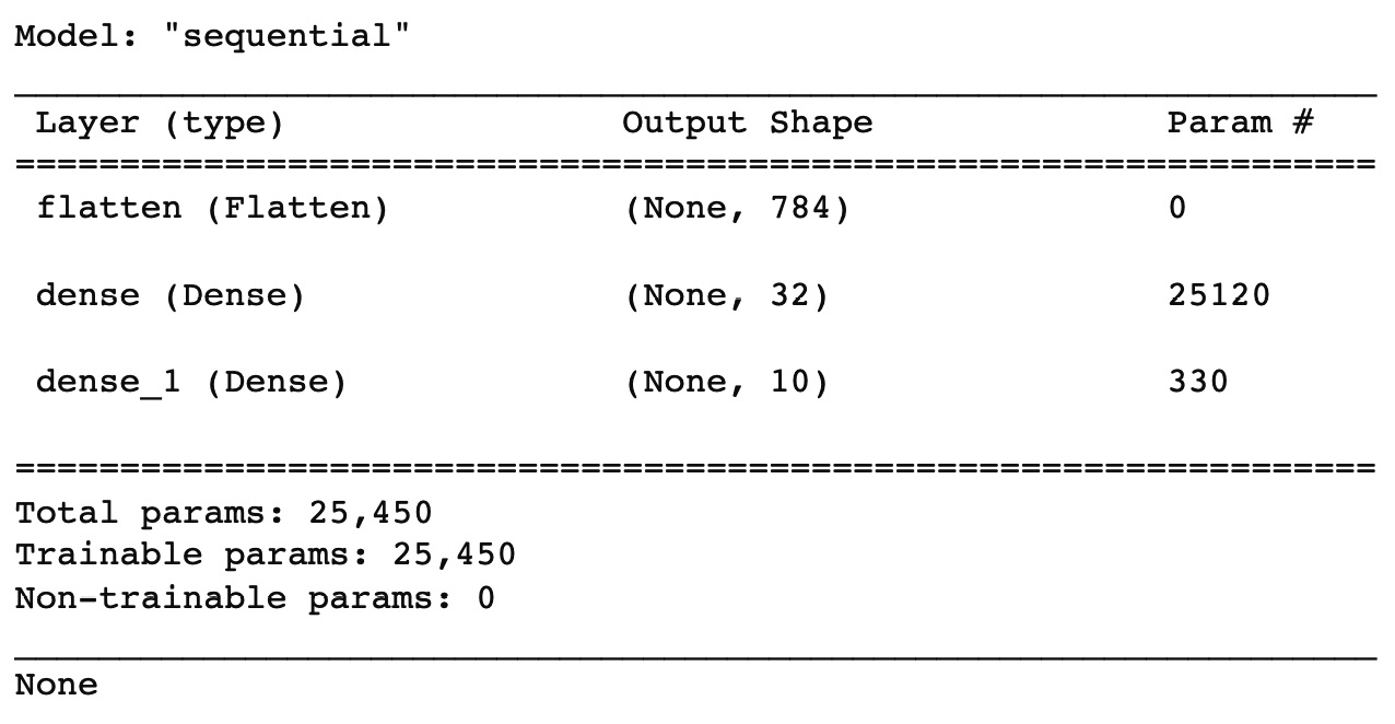
Figure 10.11 – The output of the summary() method
It is worth noting how the number of parameters and the output shape are calculated. The Flatten layer does not have any input channel. Since we have set the input shape to (28, 28), you can calculate the output shape as follows: 28 x 28 = 784. The output shape of the Flatten layer is given as input to the first Dense layer. In general, you can calculate the parameters of a Dense layer as the product between the input shape plus one (784 + 1) and the output shape plus one (32). In our case, (784 + 1) * 32 = 25,120. The output shape of the first Dense layer is given as input to the second Dense layer. Thus, you can calculate the number of parameters as follows: (32+1) * 10 = 330.
- You can plot the model graph as follows:
tf.keras.utils.plot_model(model, expand_nested=True)
The following figure shows the produced graph:

Figure 10.12 – The implemented model graph
- Comet will automatically log the training phase as well as the defined metrics. In addition, you can log the confusion matrix as follows:
preds = model.predict(test_images)
experiment.log_confusion_matrix(test_labels, preds)
First, we calculate predictions through the predict() method, then we log the confusion matrix directly in Comet.
You can also log some sample images in Comet through the summary object provided by the TensorFlow library. We log five images for the training set and five images for the test set as follows:
- We prepare the images for logging by reshaping them as follows:
train_img = np.reshape(train_images[0:5], (-1, 28, 28, 1))
test_img = np.reshape(test_images[0:5], (-1, 28, 28, 1))
- We create a file_writer object, which will store the logged images as follows:
LOG_DIR = 'logs'
file_writer = tf.summary.create_file_writer(LOG_DIR)
- We log the images:
with file_writer.as_default():
tf.summary.image("Training data", train_img, step=0)
tf.summary.image("Test data", test_img, step=0)
Now that you have built and fitted the basic model, we are ready to see the results in Comet.
Exploring results in Comet
After running the experiment, you should see the results in Comet as follows:
- Under the Chart menu, you can see the charts shown in the following figure:

Figure 10.13 – The charts automatically produced by Comet
You can access the produced charts at the following link: https://www.comet.ml/packt/deep-learning. They include the following:
- Accuracy
- Loss
- Validate batch accuracy
- Validate batch loss
- Batch loss
- Batch accuracy
- Epoch duration
- Val loss
- Val accuracy
Each graph shows the metrics versus the number of steps. Considering a default batch size of 32 and a training set of 60,000 samples, the number of steps per batch size is 60,000/32 = 1875. Since we have set the total number of epochs to 8, we can calculate the total number of steps for the training set as follows: 1875 x 8 = 15,000. For the test set (which has 10,000 samples), the number of steps per batch size is 10,000 x 32 = 312.5, which is about 313. Considering a number of epochs equal to 8, we can calculate the total number of steps for the test set as follows: 313 x 8 = 2,504. The total number of steps shown on the x-axis is given by the sum of the number of steps for the training and test phases, as follows: 15,000 + 2,504 = 17,504.
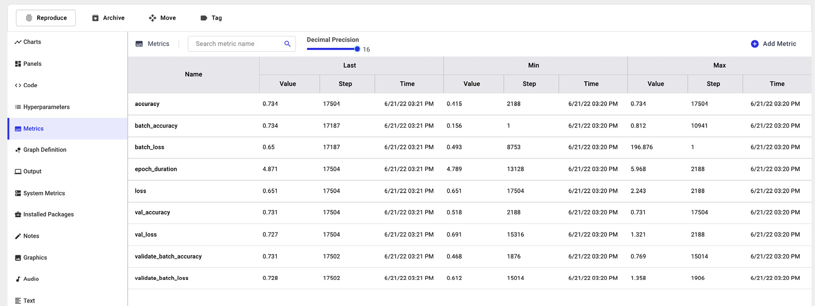
Figure 10.14 – Logged metrics in Comet
- Under the Graphics menu, you can find the examples produced through the tf.summary object, as shown in the following figure:

Figure 10.15 – Some images saved in Comet
The prefix Training data or Test data specified whether the image belongs to the training or test set, respectively.
- Under the Confusion Matrices menu, you can view the confusion matrix, as shown in the following figure:
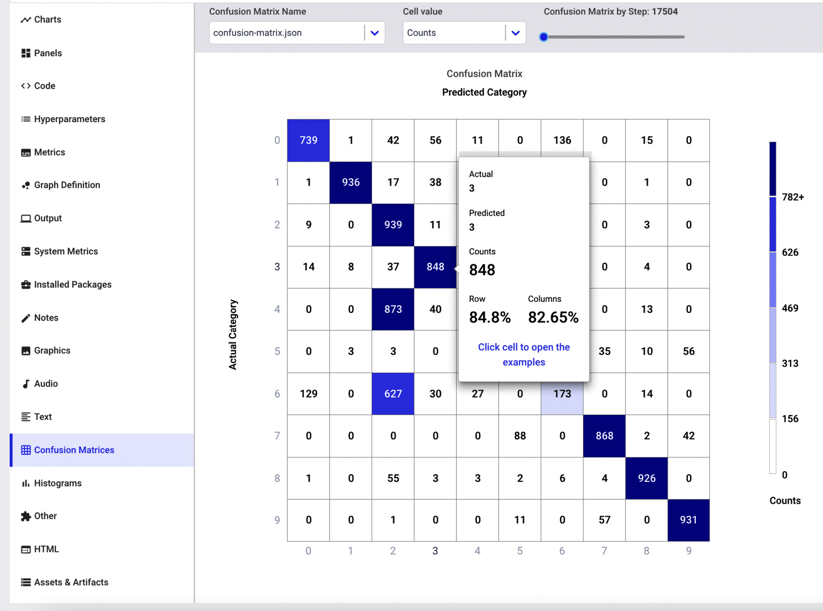
Figure 10.16 – The confusion matrix in Comet
If you move the mouse over a cell of the matrix, you will be able to see some details on the total number of values, the real ones, and the predicted ones. In addition, if you click on the cell, you will also see some examples.
- Under the Histograms menu, you can see the produced histograms, as shown in the following figure:

Figure 10.17 – The histograms in Comet
The section contains six histograms: bias, activation, and kernel for layers 2 and 3. You can see the complete graphs directly in Comet by clicking on the following link: https://www.comet.ml/packt/deep-learning, in the Histograms menu.
Now that you have explored the results in Comet, we can move on to the next step: building a prediction interface.
Building a prediction interface
You can use a prediction interface to calculate the class for an image dynamically provided as input. To build the prediction interface, we can use Gradio, a Python library, that permits you to quickly build simple interfaces for tests. In our case, the prediction interface should include an input form, where you upload an image, and an output box, which shows the predicted class. The following figure shows a possible prediction interface built in Gradio:
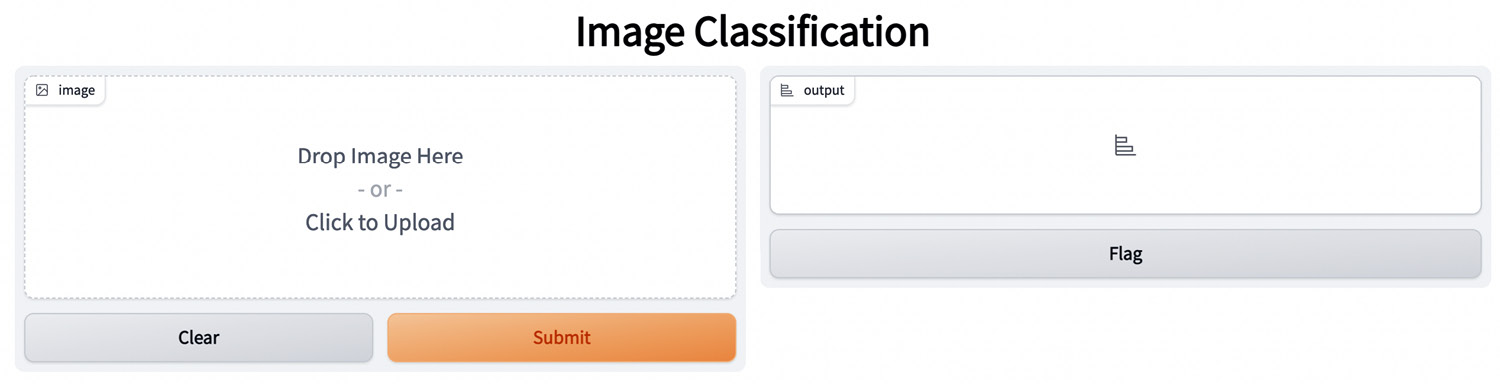
Figure 10.18 – A possible prediction interface in Gradio
Comet is fully integrated with Gradio, so you can run a Gradio interface as a Comet panel. To build the prediction interface and add it to Comet, you can perform the following steps:
- First, you need to import the Gradio library and define the Gradio interface before importing the Comet library. You can define an auxiliary function, named predict(), that calculates the predicted class for the image provided as input as follows:
import gradio as gr
model = None
def predict(image):
image = image.reshape(-1, 28, 28, 1)
prediction = model.predict(image).flatten()
return {class_names[i]: float(prediction[i]) for i in range(len(class_names))}
Since we have not defined the model yet, we initialize a dummy variable, named model, which will be set to the actual model at runtime. Here, the problem is that you must import Gradio before Comet, and TensorFlow after Comet, thus you cannot train the TensorFlow model before importing Gradio.
- Now, you can build the interface in Gradio as follows:
image = gr.inputs.Image(shape=(28, 28))
label = gr.outputs.Label()
io = gr.Interface(fn = predict,inputs = image,outputs = label, title="Image Classification")
io.launch(inline=False)
We have defined the input and the output as well as the Gradio interface. Then, we launched the interface through the launch() method, without showing it (inline = False), since we will use it in Comet.
- We create the Comet experiment as we usually do and save the experiment key because we will use it later as follows:
experiment = Experiment()
experiment_key = experiment.get_key()
We have used the get_key() method to retrieve the experiment key.
- Now, we integrate the Gradio interface in Comet as follows:
io.integrate(comet_ml=experiment)
- integrate() must be called immediately after the creation of the experiment. Unfortunately, this method also terminates the experiment, thus making it not possible to continue building the TensorFlow model. To overcome this issue, we reopen the experiment by creating an ExistingExperiment object as follows:
from comet_ml import ExistingExperiment
experiment = ExistingExperiment(previous_experiment=experiment_key)
To create an ExistingExperiment object, you need to pass the key of the preceding experiment. The ExistingExperiment object continues the preceding experiment.
- After reopening the experiment, you can continue working on it by creating and training your TensorFlow model as described in the preceding section.
Once you have run the experiment, you can access the Comet dashboard and create a new panel with the Gradio interface. To create the Gradio panel, you can perform the following steps:
- From the Comet project main dashboard, select the Panels tab, then Add | New Panel | PUBLIC | Gradio Panel | Add | Done.
- You should see a new panel in your Comet dashboard as shown in the following figure:

Figure 10.19 – The Gradio interface
In the preceding example, we uploaded an image representing a shirt (shown on the left), and our predictor returned the T-shirt/top with a probability of 38% and the Shirt class with a probability of 24%.
Now that you have built the Gradio interface, you can move on to the final step: building the final report.
Building the final report
Now you are ready to build the final report. In this example, we build a simple report with the model results. As a further exercise, you could improve them by applying the concepts learned in Chapter 5,Building a Narrative in Comet.
To create the report, in the Comet dashboard you can click on the Panels tab, then select Add | Add to Report | New Report.
You will create a report with the following three sections:
- Data
- Model evaluation
- Real-time prediction
The report automatically loads the model evaluation report; thus, we will describe only how to build the first and the third sections. Let’s start with the first section: data.
Data
Let’s begin by performing the following steps:
- First, we need to create a new section by clicking on the Add section here button, which is available when you hover the mouse at the top of the previous section.
- Then, we insert the logged sample images. We use the Comet Viewer Panel, which you can add by clicking on Add | New Panel | PUBLIC | Comet Viewer Panel | Add | Done.
The following figure shows the produced Comet Viewer Panel:
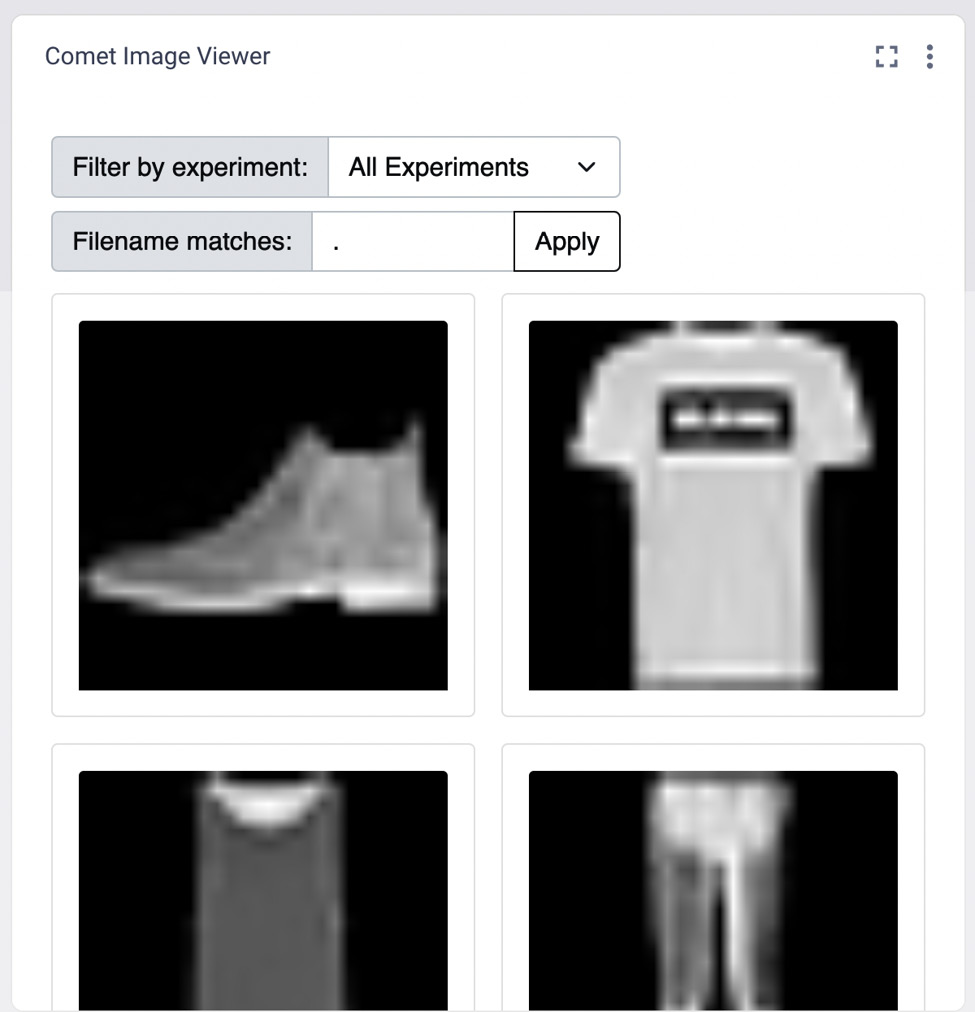
Figure 10.20 – The Comet Viewer Panel
The panel permits you to filter images by experiments. In our case, we have just one experiment, thus the panel automatically shows it.
Real-time prediction
In this section, we add the Gradio panel as follows:
- First, we create a new section by clicking the Add section here button, which is available when you hover the mouse at the bottom of the Model Evaluation section.
- Then, we add a new panel, as described in the Building a prediction interface section of this chapter.
Your report is ready! You can view the final result directly in Comet at the following link: https://www.comet.ml/packt/deep-learning/reports/clothes-classification.
Summary
We have just completed the journey to build a deep learning model in TensorFlow and track it in Comet!
Throughout this chapter, we described some general concepts regarding deep learning as well as the main structure of the TensorFlow package, and some related concepts, including how to load a dataset and build and train a model in TensorFlow.
In the last part of the chapter, we implemented a practical use case that showed you how to track a deep learning experiment in Comet as well as how to build a report with the results of the experiment.
In the next chapter, we will review the basic concepts related to time series analysis and how to perform it in Comet.
Further reading
- Gulli, A., Kapoor, A., and Pal, S. (2019). Deep Learning with TensorFlow 2 and Keras: Regression, ConvNets, GANs, RNNs, NLP, and More with TensorFlow 2 and the Keras API. Packt Publishing Ltd.
- Ramsundar, B., and Zadeh, R. B. (2018). TensorFlow for Deep Learning: From Linear Regression to Reinforcement Learning. O’Reilly Media, Inc.
- Tung, KC (2021). TensorFlow 2 Pocket Reference. O’Reilly Media, Inc.