Chapter 8: Putting It All Together

In this chapter, we will revisit the Lending Club Loan Application data that we first introduced in Chapter 3, Fundamental Workflow – Data to Deployable Model. This time, we begin the way most data science projects do, that is, with a raw data file and a general objective or question. Along the way, we will refine both the data and the problem statements so that they are relevant to the business and can be answered by the available data. Data scientists rarely begin with modeling-ready data; therefore, the treatment in this chapter more accurately reflects the job of a data scientist in the enterprise. We will then model the data and evaluate various candidate models, updating them as required, until we arrive at a final model. We will evaluate the final model and illustrate the preparation steps required for model deployment. This reinforces what we introduced in Chapter 5 through Chapter 7.

By the end of this chapter, you will be able to take an unstructured problem with a raw data source and create a deployable model to answer a refined predictive question. For completeness, we will include all the code required to do each step of data preparation, feature engineering, model building, and evaluation. In general, any code that has already been covered in Chapter 5 through Chapter 7 will be left uncommented.

This chapter is divided into four sections, each of which has individual steps. The sections are listed as follows:

• Data wrangling
• Feature engineering
• Model building and evaluation
• Preparation for model pipeline deployment

Technical requirements

If you still have not set up your H2O environment at this stage, to do so, please see Appendix – Alternative Methods to Launch H2O Clusters.

Data wrangling

It is frequently said that 80–90% of a data scientist's job is dealing with data. At a minimum, you should understand the data granularity (that is, what the rows represent) and know what each column in the dataset means. Presented with a raw data source, there are multiple steps required to clean, organize, and transform your data into a modeling-ready dataset format.

The dataset used for the Lending Club example in Chapters 3, 5, and 7 was derived from a raw data file that we begin with here. In this section, we will illustrate the following steps:

1. Import the raw data and determine which columns to keep.
2. Define the problem, and create a response variable.
3. Convert the implied numeric data from strings into numeric values.
4. Clean up any messy categorical columns.

Let's begin with the first step: importing the data.

Importing the raw data

We import the raw data file using the following code:

input_csv = "rawloans.csv"

loans = h2o.import_file(input_csv,

             col_types = {"int_rate": "string",

                          "revol_util": "string",

                          "emp_length": "string",

                          "verification_status": "string"})

A dictionary in the h2o.import_file code specifies the input column type of string for four of the input variables: int_rate, revol_util, emp_length, and verification_status. Specifying the column type explicitly ensures that the column is read in as the modeler intended. Without this code, these string variables might have been read as categorical columns with multiple levels.

The dataset dimensions are obtained by the following command:

loans.dim

This returns 42,536 rows (corresponding to 42,536 customer credit applications) and 52 columns. Next, we specify the 22 columns we wish to keep for our analysis:

keep = ['addr_state', 'annual_inc', 'delinq_2yrs',

        'dti', 'earliest_cr_line', 'emp_length', 'grade',

        'home_ownership', 'inq_last_6mths', 'installment',

        'issue_d', 'loan_amnt', 'loan_status',

        'mths_since_last_delinq', 'open_acc', 'pub_rec',

        'purpose', 'revol_bal', 'revol_util', 'term',

        'total_acc', 'verification_status']

And we want to remove the remaining columns using the drop method:

remove = list(set(loans.columns) - set(keep))

loans = loans.drop(remove)

But what about the 30 columns that we removed? They contained things such as text descriptions of the purpose of the loan, additional customer information such as the address or zip code, columns with almost completely missing information or other data quality issues, and more. Selecting the appropriate columns from a raw data source is an important task that takes much time and effort on the part of the data scientist.

The columns we keep are those we believe are most likely to be predictive. Explanations for each column are listed as follows:

• addr_state: This is the US state where the borrower resides.
• annual_inc: This is the self-reported annual income of the borrower.
• delinq_2yrs: This is the number of times the borrower has been more than 30 days late in payments during the last 2 years.
• dti: This is the debt-to-income ratio (current debt divided by income).
• earliest_cr_line: This is the date of the earliest credit line (generally, longer credit histories correlate with better credit risk).
• emp_length: This is the length of employment.
• grade: This is a risk rating from A to G assigned to the loan by the lender.
• home_ownership: Does the borrower own a home or rent?
• inq_last_6mths: This is the number of credit inquiries in the last 6 months.
• installment: This is the monthly amount owed by the borrower.
• issue_d: This is the date the loan was issued.
• loan_amnt: This is the total amount lent to the borrower.
• loan_status: This is a category.
• mths_since_last_delinq: This is the number of months since the last delinquency.
• open_acc: This is the number of open credit lines.
• pub_rec: This is the number of derogatory public records (bankruptcies, tax liens, and judgments).
• purpose: This is the borrower's stated purpose for the loan.
• revol_bal: This is the revolving balance (that is, the amount owed on credit cards at the end of the billing cycle).
• revol_util: This is the revolving utilization (that is, the amount of credit used divided by the total credit available to the borrower).
• term: This is the number of payments on the loan in months (either 36 or 60).
• total_acct: This is the borrower's total number of credit lines.
• verification_status: This tells us whether the income was verified or not.

Assuming our data columns have been properly selected, we can move on to the next step: creating the response variable.

Defining the problem and creating the response variable

The creation of the response variable depends on the problem definition. The goal of this use case is to predict which customers will default on a loan. A model that predicts a loan default needs a response variable that differentiates between good and bad loans. Let's start by investigating the loan_status variable using the following code:

loans["loan_status"].table().head(20)

This produces a table with all possible values of the loan status stored in our data:

Figure 8.1 – Loan status categories from the raw Lending Club loan default dataset

As you can see in Figure 8.1, the loan_status variable is relatively complex, containing 11 categories that are somewhat redundant or overlapping. For instance, Charged Off indicates that 5,435 loans were bad. Default contains another 7. Fully Paid shows that 30,843 loans were good. Some loans, for example, those indicated by the Current or Late categories, are still ongoing and so are not yet good or bad.

Multiple loans were provided that did not meet the credit policy. Why this was allowed is unclear and worth checking with the data source. Did the credit policy change so that these loans are of an earlier vintage? Are these formal overrides or were they accidental? Whatever the case might be, these categories hint at a different underlying population that might require our attention. Should we remove these loans altogether, ignore the issue by collapsing them into their corresponding categories, or create a Meets Credit Policy indicator variable and model them directly? A better understanding of the data would allow the data scientist to make an informed decision.

In the end, we need a binary response variable based on a population of loans that have either been paid off or defaulted. First, filter out any ongoing loans.

Removing ongoing loans

We need to build our model with only those loans that have either defaulted or been fully paid off. Ongoing loans have loan_status such as Current or In Grace Period. The following code captures the rows whose statuses indicate ongoing loans:

ongoing_status = [

    "Current",

    "In Grace Period",

    "Late (16-30 days)",

    "Late (31-120 days)",

    "Does not meet the credit policy.  Status:Current",

    "Does not meet the credit policy.  Status:In Grace Period"

]

We use the following code to remove those ongoing loans and display the status for the remaining loans:

loans = loans[~loans["loan_status"].isin(ongoing_status)]

loans["loan_status"].table()

The resulting status categories are shown in Figure 8.2:

Figure 8.2 – Loan status categories after filtering the ongoing loans

Note that, in Figure 8.2, five categories of loan status now need to be summarized in a binary response variable. This is detailed in the next step.

Defining the binary response variable

We start by forming a fully_paid list to summarize the loan status categories:

fully_paid = [

    "Fully Paid",

    "Does not meet the credit policy.  Status:Fully Paid"

]

Next, let's create a binary response column, bad_loan, as an indicator for any loans that were not completely paid off:

response = "bad_loan"

loans[response] = ~(loans["loan_status"].isin(fully_paid))

loans[response] = loans[response].asfactor()

Finally, remove the original loan status column:

loans = loans.drop("loan_status")

We remove the original loan status column because the information we need for building our predictive model is now contained in the bad_loan response variable.

Next, we will convert string data into numeric values.

Converting implied numeric data from strings into numeric values

There are various ways that data can be messy. In the preceding step, we saw how variables can sometimes contain redundant categories that might benefit from summarization. The format in which data values are displayed and stored can also cause problems. Therefore, the 28% that we naturally interpret as a number is, typically, input as a character string by a computer. Converting implied numeric data into actual numeric data is a very typical data quality task.

Consider the revol_util and emp_length columns:

loans[["revol_util", "emp_length"]].head()

The output is shown in the following screenshot:

Figure 8.3 – Variables stored as strings to be converted into numeric values

The revol_util variable, as shown in Figure 8.3, is inherently numeric but has a trailing percent sign. In this case, the solution is simple: strip the % sign and convert the strings into numeric values. This can be done with the following code:

x = "revol_util"

loans[x] = loans[x].gsub(pattern="%", replacement="")

loans[x] = loans[x].trim()

loans[x] = loans[x].asnumeric()

The gsub method substitutes % with a blank space. The trim method removes any whitespace in the string. The asnumeric method converts the string value into a number.

The emp_length column is only slightly more complex. First, we need to strip out the year or years term. Also, we must deal with the < and + signs. If we define < 1 as 0 and 10+ as 10, then emp_length can also be cast as numeric. This can be done using the following code:

x = "emp_length"

loans[x] = loans[x].gsub(pattern="([ ]*+[a-zA-Z].*)|(n/a)", 

                         replacement="") 

loans[x] = loans[x].trim()

loans[x] = loans[x].gsub(pattern="< 1", replacement="0")

loans[x] = loans[x].gsub(pattern="10\+", replacement="10") 

loans[x] = loans[x].asnumeric()

Next, we will complete our data wrangling steps by cleaning up any messy categorical columns.

Cleaning up messy categorical columns

The last step in preparation for feature engineering and modeling is clarifying the options or levels in often messy categorical columns. This standardization task is illustrated by the verification_status variable. Use the following code to find the levels of verification_status:

loans["verification_status"].head()

The results are displayed in Figure 8.4:

Figure 8.4 – The categories of the verification status from the raw data

Because there are multiple values in Figure 8.4 that mean verified (VERIFIED - income and VERIFIED - income source), we simply replace them with verified. The following code uses the sub method for easy replacement:

x = "verification_status"

loans[x] = loans[x].sub(pattern = "VERIFIED - income source",

                        replacement = "verified")

loans[x] = loans[x].sub(pattern = "VERIFIED - income",

                        replacement = "verified")

loans[x] = loans[x].asfactor()

After completing all our data wrangling steps, we will move on to feature engineering.

Feature engineering

In Chapter 5, Advanced Model Building – Part I, we introduced some feature engineering concepts and discussed target encoding at length. In this section, we will delve into feature engineering in a bit more depth. We can organize feature engineering as follows:

• Algebraic transformations
• Features engineered from dates
• Simplifying categorical variables by combining categories
• Missing value indicator functions
• Target encoding categorical columns

The ordering of these transformations is not important except for the last one. Target encoding is the only transformation that requires data to be split into train and test sets. By saving it for the end, we can apply the other transformations to the entire dataset at once rather than separately to the training and test splits. Also, we introduce stratified sampling for splitting data in H2O-3. This has very little impact on our current use case but is important when data is highly imbalanced, such as in fraud modeling.

In the following sections, we include all our feature engineering code for completeness. Code that has been introduced earlier will be merely referenced, while new feature engineering tasks will merit discussion. Let's begin with algebraic transformations.

Algebraic transformations

The most straightforward form of feature engineering entails taking simple transformations of the raw data columns: the log, the square, the square root, the differences in columns, the ratios of the columns, and more. Often, the inspiration for these transformations comes from an underlying theory or is based on subject-matter expertise.

The credit_length variable, as defined in Chapter 5, Advanced Model Building – Part I, is one such transformation. Recall that this is created with the following code:

loans["credit_length"] = loans["issue_d"].year() - 

    loans["earliest_cr_line"].year()

The justification for this variable is based on a business observation: customers with longer credit histories tend to be at lower risk of defaulting. Also, we drop the earliest_cr_line variable, which is no longer needed:

loans = loans.drop(["earliest_cr_line"])

Another simple feature we could try is (annual income)/(number of credit lines), taking the log for distributional and numerical stability. Let's name it log_inc_per_acct. This ratio makes intuitive sense: larger incomes should be able to support a greater number of credit lines. This is similar to the debt-to-income ratio in intent but captures slightly different information. We can code it as follows:

x = "log_inc_per_acct"

loans[x] = loans['annual_inc'].log() - 

    loans['total_acc'].log()

Next, we will consider the second feature engineering task: encoding information from dates.

Features engineered from dates

As noted in Chapter 5, Advanced Model Building – Part I, there is a wealth of information contained in date values that are potentially predictive. To the issue_d_year and issue_d_month features that we created earlier, we add issue_d_dayOfWeek and issue_d_weekend as new factors. The code to do this is as follows:

x = "issue_d"

loans[x + "_year"] = loans[x].year()

loans[x + "_month"] = loans[x].month().asfactor()

loans[x + "_dayOfWeek"] = loans[x].dayOfWeek().asfactor()

weekend = ["Sat", "Sun"]

loans[x + "_weekend"] = loans[x + "_dayOfWeek"].isin(weekend)

loans[x + "_weekend"] = loans[x + "_weekend"].asfactor()

At the end, we drop the original date variable:

loans = loans.drop(x)

Next, we will address how to simplify categorical variables at the feature engineering stage.

Simplifying categorical variables by combining categories

In the data wrangling stage, we cleaned up the messy categorical levels for the verification_status column, removing redundant or overlapping level definitions and making categories mutually exclusive. On the other hand, during this feature engineering stage, the category levels are already non-overlapping and carefully defined. The data values themselves, for instance, small counts for certain categories, might suggest some engineering approaches to improve predictive modeling.

Summarize the home_ownership categorical variable using the following code:

x = "home_ownership"

loans[x].table()

The tabled results are shown in the following screenshot:

Figure 8.5 – Levels of the raw home ownership variable

In Figure 8.5, although there are five recorded categories within home ownership, the largest three have thousands of observations: MORTGAGE, OWN, and RENT. The remaining two, NONE and OTHER, are so infrequent (8 and 135, respectively) that we will combine them with OWN to create an expanded OTHER category.

Collapsing Data Categories

Depending on the inference we want to make, or our understanding of the problem, it might make more sense to collapse NONE and OTHER into the RENT or MORTGAGE categories.

The procedure for combining the categorical levels is shown by the following command:

loans[x].levels()

This is given by replacing the NONE and OWN level descriptions with OTHER and assigning it to a new variable, home_3cat, as shown in the following code:

lvls = ["MORTGAGE", "OTHER", "OTHER", "OTHER", "RENT"]

loans["home_3cat"] = 

    loans[x].set_levels(lvls).ascharacter().asfactor()

Then, we drop the original home_ownership column:

loans = loans.drop(x)

Next, we will visit how to create useful indicator functions for missing data.

Missing value indicator functions

When data is not missing at random, the pattern of missingness might be a source of predictive information. In other words, sometimes, the fact that a value is missing is as, or more, important than the actual value itself. Especially in cases where missing values are abundant, creating a missing value indicator function can prove helpful.

The most interesting characteristic of employment length, emp_length, is whether the value for a customer is missing. Simple pivot tables show that the proportion of bad loans is 26.3% for customers with missing emp_length values and 18.0% for non-missing values. That disparity in default rates suggests using a missing value indicator function as a predictor.

The code for creating a missing indicator function for the emp_length variable is simple:

loans["emp_length_missing"] = loans["emp_length"] == None

Here, the new emp_length_missing column contains the indicator function. Unlike the other features that we engineered earlier, the original emp_length column does not need to be dropped as a possible predictor.

Next, we will turn to target encoding categorical columns.

Target encoding categorical columns

In Chapter 5, Advanced Model Building – Part I, we introduced target encoding in H2O-3 in some detail. As a prerequisite to target encoding, recall that a train and test set was required. We split the data using the split_frame method with code similar to the following:

train, test = loans.split_frame(ratios = [0.8], seed = 12345)

The split_frame method creates a completely random sample split. This approach is required for all regression models and works well for relatively balanced classification problems. However, when binary classification is highly imbalanced, stratified sampling should be used instead.

Stratified sampling for binary classification data splits

Stratified sampling for binary classification works by separately sampling the good and bad loans. In other words, recall that 16% of the loans in our Lending Club dataset are bad. We wish to split the data into 80% train and 20% test datasets. If we separately sample 20% of the bad loans and 20% of the good loans and then combine them, we have a test dataset that preserves the 16% bad loan percentage. Combining the remaining data results in a 16% bad loan percentage in our training data. Therefore, stratified sampling preserves the original category ratios.

We use the stratified_split method on the response column to create a new variable named split, which contains the train and test values, as shown in the following code:

loans["split"] = loans[response].stratified_split(

    test_frac = 0.2, seed = 12345)

loans[[response,"split"]].table()

The results of the stratified split are shown in the following screenshot:

Figure 8.6 – The stratified split of loan data into train and test

We use the split column to create a Boolean mask for deriving the train and test datasets, as shown in the following code:

mask = loans["split"] == "train"

train = loans[mask, :].drop("split")

test = loans[~mask, :].drop("split")

Note that we drop the split column from both datasets after their creation. Now we are ready to target encode using these train and test splits.

Target encoding the Lending Club data

The following code for target encoding the purpose and addr_state variables is similar to the code from Chapter 5, Advanced Model Building – Part I, which we have included here without discussion:

from h2o.estimators import H2OTargetEncoderEstimator

encoded_columns = ["purpose", "addr_state"]

train["fold"] = train.kfold_column(n_folds = 5, seed = 25)

te = H2OTargetEncoderEstimator(

    data_leakage_handling = "k_fold",

    fold_column = "fold",

    noise = 0.05,

    blending = True,

    inflection_point = 10,

    smoothing = 20)

te.train(x = encoded_columns,

         y = response,

         training_frame = train)

train_te = te.transform(frame = train)

test_te = te.transform(frame = test, noise = 0.0)

Next, we redefine the train and test datasets, dropping the encoded columns from the target-encoded train_te and test_te splits. Also, we also drop the fold column from the train_te dataset (note that it does not exist in the test_te dataset). The code is as follows:

train = train_te.drop(encoded_columns).drop("fold")

test = test_te.drop(encoded_columns)

With our updated train and test datasets, we are ready to tackle the model building and evaluation processes.

Model building and evaluation

Our approach to model building starts with AutoML. Global explainability applied to the AutoML leaderboard either results in picking a candidate model or yields insights that we feed back into a new round of modified AutoML models. This process can be repeated if improvements in modeling or explainability are apparent. If a single model rather than a stacked ensemble is chosen, we can show how an additional random grid search could produce better models. Then, the final candidate model is evaluated.

The beauty of this approach in H2O-3 is that the modeling heavy lifting is done for us automatically with AutoML. Iterating through this process is straightforward, and the improvement cycle can be repeated, as needed, until we have arrived at a satisfactory final model.

We organize the modeling steps as follows:

1. Model search and optimization with AutoML.
2. Investigate global explainability with the AutoML leaderboard models.
3. Select a model from the AutoML candidates, with an optional additional grid search.
4. Final model evaluation.

Model search and optimization with AutoML

The model build process using H2O-3 AutoML was extensively introduced in Chapter 5, Advanced Model Building – Part I. Here, we will follow a virtually identical process to create a leaderboard of models fit by AutoML. For clarity, we redefine our response column and predictors before removing the bad_loan response from the set of predictors:

response = "bad_loan"

predictors = train.columns

predictors.remove(response)

Our AutoML parameters only exclude deep learning models, allowing the process to run for up to 30 minutes, as shown in the following code snippet:

from h2o.automl import H2OAutoML

aml = H2OAutoML(max_runtime_secs = 1800,

                exclude_algos = ['DeepLearning'],

                seed = 12345)

aml.train(x = predictors, 

          y = response, 

          training_frame = train)

As demonstrated in Chapter 5, Advanced Model Building – Part I, we can access H2O Flow to monitor the model build process in more detail. Once the training on the aml object finishes, we proceed to investigate the resulting models with global explainability.

Investigating global explainability with AutoML models

In Chapter 7, Understanding ML Models, we outlined the use of global explainability for a series of models produced by AutoML. Here, we will follow the same procedure by calling the explain method with the test data split:

aml.explain(test)

The resulting AutoML leaderboard is shown in the following screenshot:

Figure 8.7 – The top 10 models of the AutoML leaderboard

The stacked ensemble AllModels and BestOfFamily models claim the top two positions on the leaderboard in Figure 8.7. The best single model is enclosed by a green box and labeled model_6 from XGBoost_grid__1. We will investigate this model a bit further as a possible candidate model.

The Model Correlation plot is shown in Figure 8.8. The green box indicates the correlation between our candidate XGBoost model and the two stacked ensembles. It confirms that the candidate model has among the highest correlation with the ensembles:

Figure 8.8 – Model Correlation plot for the AutoML leaderboard models

The Variable Importance Heatmap diagram in Figure 8.9 tells us more about the stability of the individual features than about the relationship between the models. The GBM grid models of 1, 2, 3, and 7 cluster together, and the XGBoost grid models of 6, 7, and 9 appear very similar in terms of how important variables are in these models:

Figure 8.9 – Variable Importance Heatmap for AutoML models

The multiple model Partial Dependence Plots (PDPs), in conjunction with the variable importance heatmap, yield some valuable insights. Figure 8.10 shows the PDP for grade, a feature with values from A to G that appear to be increasing at default risk. In other words, the average response for A is less than that for B, which is itself less than that for C, and so forth. This diagnostic appears to be confirming a business rating practice:

Figure 8.10 – The multiple model PDP for grade

In Figure 8.11, the PDP for annual income acts as a diagnostic. Intuitively, an increase in annual income should correspond to a decrease in bad loan rates. We can formally enforce (rather than just hope for) a monotonic decreasing relationship between the annual income and the default rate by adding monotonicity constraints to our model build code:

Figure 8.11 – The multiple model PDP for annual income

Monotonicity constraints can be applied to one or more numeric variables in the GBM, XGBoost, and AutoML models in H2O-3. To do so, supply a monotone_constraints parameter with a dictionary of variable names and the direction of the monotonicity: 1 for a monotonic increasing relationship and -1 for monotonic decreasing. The following code shows how we add a monotonic decreasing annual_inc constraint:

maml = H2OAutoML(

         max_runtime_secs = 1800,

         exclude_algos = ['DeepLearning'],

         monotone_constraints = {"annual_inc": -1}, 

         seed = 12345)

Monotonic Increasing and Decreasing Constraints

Formally, the monotonic increasing constraint is a monotonic non-decreasing constraint, meaning that the function must either be increasing or flat. Likewise, the monotonic decreasing constraint is more correctly termed a monotonic non-increasing constraint.

Fitting a constrained model proceeds as usual:

maml.train(x = predictors, 

           y = response, 

           training_frame = train)

Here is the explain method:

maml.explain(test)

This produces the leaderboard, as shown in the following screenshot:

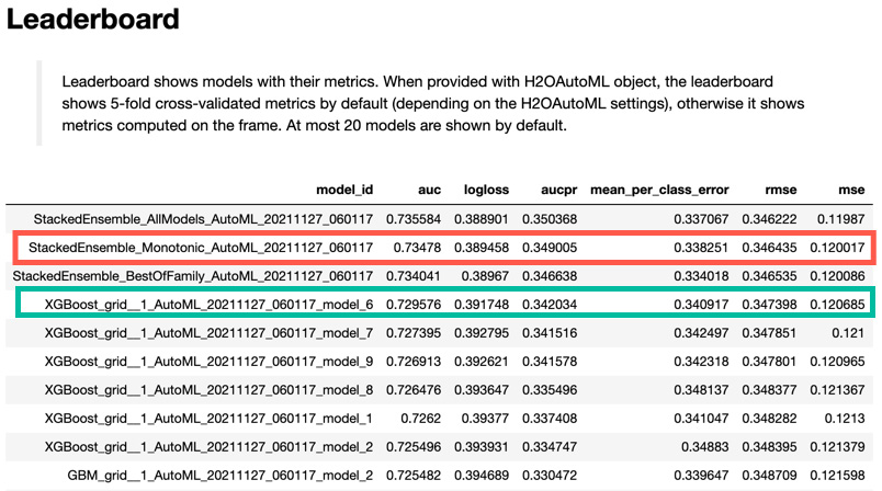
Figure 8.12 – The leaderboard for AutoML with monotonic constraints

The first 10 models of the updated AutoML leaderboard are shown in Figure 8.12. Note that a new model has been added, the monotonic stacked ensemble (boxed in red). This stacked ensemble uses, as constituent models, only those that are monotonic. In our case, this means that any DRF and XRT random forest models fit by AutoML would be excluded. Also note that the monotonic version of XGBoost model 6 is once more the leading single model, boxed in green.

Figure 8.13 shows the monotonic multiple model PDP for annual income:  

Figure 8.13 – The multiple model PDP for annual income

Note that only two of the models included in the PDP of Figure 8.13 are not monotonic: the DRF and XRT models. They are both versions of random forest that do not have monotonic options. This plot confirms that the monotonic constraints on annual income worked as intended. (Note that the PDP in Figure 8.11 is very similar. The models there might have displayed monotonicity, but it was not enforced.)

Next, we will consider how to choose a model from the AutoML leaderboard.

Selecting a model from the AutoML candidates

Once AutoML has created a class of models, it is left to the data scientist to determine which model to put into production. If pure predictive accuracy is the only requirement, then the choice is rather simple: select the top model in the leaderboard (usually, this is the All Models stacked ensemble). In the case where monotonic constraints are required, the monotonic stacked ensemble is usually the most predictive.

If business or regulatory constraints only allow a single model to be deployed, then we can select one based on a combination of predictive performance and other considerations, such as the modeling type. Let's select XGBoost model 6 as our candidate model:

candidate = h2o.get_model(maml.leaderboard[3, 'model_id'])

H2O-3 AutoML does a tremendous job at building and tuning models across multiple modeling types. For individual models, it is sometimes possible to get an improvement in performance via an additional random grid search. We will explore this in the next section.

Random grid search to improve the selected model (optional)

We use the parameters of the candidate model as starting points for our random grid search. The idea is to search within the neighborhood of the candidate model for models that perform slightly better, noting that any improvements found will likely be minor. The stacked ensemble models give us a ceiling for how well an individual model can perform. The data scientist must judge whether the difference between candidate model performance and stacked ensemble performance warrants the extra effort in searching for possibly better models.

We can list the model parameters using the following code:

candidate.actual_params

Start by importing H2OGridSearch and the candidate model estimator; in our case, that is H2OXGBoostEstimator:

from h2o.grid.grid_search import H2OGridSearch

from h2o.estimators import H2OXGBoostEstimator

The hyperparameters are selected by looking at the candidate model's actual parameters and searching within the neighborhood of those values. For instance, the sample rate for the candidate model was reported as 80%, and in our hyperparameter tuning, we select a range between 60% and 100%. Likewise, a 60% column sample rate leads us to implement a range between 40% and 80% for the grid search. The hyperparameter tuning code is as follows:  

hyperparams_tune = {

    'max_depth' : list(range(2, 6, 1)),

    'sample_rate' : [x/100. for x in range(60,101)],

    'col_sample_rate' : [x/100. for x in range(40,80)],

    'col_sample_rate_per_tree': [x/100. for x in

         range(80,101)],

    'learn_rate' : [x/100. for x in range(5,31)]

}

We limit the overall runtime of the random grid search to 30 minutes, as follows:

search_criteria_tune = {

    'strategy' : "RandomDiscrete",

    'max_runtime_secs' : 1800,

    'stopping_rounds' : 5,

    'stopping_metric' : "AUC",

    'stopping_tolerance': 5e-4

}

We add the monotonic constraints to the model and define our grid search:

monotone_xgb_grid = H2OXGBoostEstimator(

    ntrees = 90,

    nfolds = 5,

    score_tree_interval = 10,

    monotone_constraints = {"annual_inc": -1},

    seed = 25)

monotone_grid = H2OGridSearch(

    monotone_xgb_grid,

    hyper_params = hyperparams_tune,

    grid_id = 'monotone_grid',

    search_criteria = search_criteria_tune)

Then, we train the model:

monotone_grid.train(

    x = predictors,

    y = response,

    training_frame = train)

Returning to our results after this long training period, we extract the top two models to compare them with our initial candidate model. Note that we order by logloss:

monotone_sorted = monotone_grid.get_grid(sort_by = 'logloss',

                                         decreasing = False)

best1 = monotone_sorted.models[0]

best2 = monotone_sorted.models[1]

Determine the performance of each of these models on the test data split:

candidate.model_performance(test).logloss()

best1.model_performance(test).logloss()

best2.model_performance(test).logloss()

On the test sample, the logloss for the candidate model is 0.3951, best1 is 0.3945, and best2 is 0.3937. Based on this criterion alone, the best2 model is our updated candidate model. The next step is the evaluation of this final model.

Final model evaluation

Having selected best2 as our final candidate, next, we evaluate this individual model using the explain method:

final = best2

final.explain(test)

We will use the variable importance plot in Figure 8.14 in conjunction with individual PDPs to understand the impact of the input variables on this model:

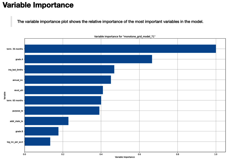
Figure 8.14 – Variable importance for the final model

The term variable is by far the most important variable in the final model. Inspecting the PDP for "term" in Figure 8.15 explains why.

Figure 8.15 – PDP for term

Loans with a term of 36 months have a default rate of around 12%, while 60-month loans have a default rate that jumps to over 25%. Note that because this is an XGBoost model, term was parameterized as term 36 months.

The next variable in importance is grade A. This is an indicator function for one level of the categorical grade variable. Looking at the PDP for grade in Figure 8.16, loans with a level of A only have a 10% default rate with an approximate 5% jump for the next lowest risk grade, B:

Figure 8.16 – PDP for grade

The next two variables are numeric and roughly equivalent in importance: credit inquiries in the last 6 months (inq_last_6mths) and annual income. Their PDPs are shown in Figures 8.17 and Figure 8.18, respectively. The credit inquiries PDP appears to be monotonic except for the right-hand tail. This is likely due to thin data in this upper region of high numbers of inquiries. It would probably make sense to add a monotonic constraint to this variable as we did for annual income in Figure 8.18:

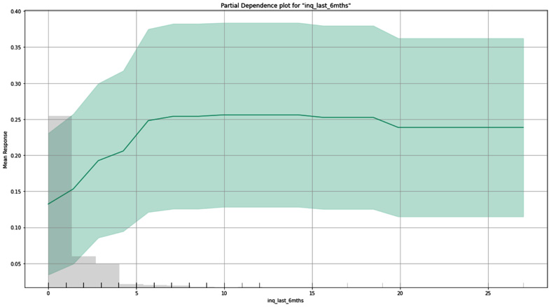
Figure 8.17 – PDP for the number of inquiries in the last 6 months

Figure 8.18 – PDP for monotonic annual income

Figure 8.19 shows the PDP for revolving credit utilization. Unlike earlier numeric plots, the revol_util variable is not visibly monotonic. In general, the higher the utilization, the greater the default rate. However, there is a relatively high default rate at the utilization of zero. Sometimes, effects such as this are caused by mixtures of disparate populations. For example, this could be a combination of customers who have credit lines but carry no balances (generally good risks) with customers who have no credit lines at all (generally poorer risks). Without reparameterization, revol_util should not be constrained to be monotonic:

Figure 8.19 – PDP for revolving utilization

Finally, Figure 8.20 shows the SHAP summary for the final model. The relative importance in terms of SHAP values is slightly different than that of our feature importance and PDP views:

Figure 8.20 – The SHAP Summary plot for the final model

This has been a taster of what a final model review or whitepaper would show. Some of these are multiple pages in length.

Preparation for model pipeline deployment

Exporting a model as a MOJO for final model deployment is trivial, for instance, consider the following:

final.download_MOJO("final_MOJO.zip")

Deployment of the MOJO in various architectures via multiple recipes is covered, in detail, in Chapter 9, Production Scoring and the H2O MOJO. In general, there is a significant amount of effort that must be assigned to productionizing data for model scoring. The key is that data used in production must have a schema identical to that of the training data used in modeling. In our case, that means all the data wrangling and feature engineering tasks must be productionized before scoring in production can occur. In other words, the process is simply as follows:

1. Transform raw data into the training data format.
2. Score the model using the MOJO on the transformed data.

It is a best practice to work with your DevOps or equivalent production team well in advance of model delivery to understand the data requirements for deployment. This includes specifying roles and responsibilities such as who is responsible for producing the data transformation code, how is the code to be tested, who is responsible for implementation, and more. Usually, the delivery of a MOJO is not the end of the effort for a data science leader. We will discuss the importance of this partnership, in more detail, in Chapter 9, Production Scoring and the H2O MOJO.

Summary

In this chapter, we reviewed the entire data science model-building process. We started with raw data and a somewhat vaguely defined use case. Further inspection of the data allowed us to refine the problem statement to one that was relevant to the business and that could be addressed with the data at hand. We performed extensive feature engineering in the hopes that some features might be important predictors in our model. We introduced an efficient and powerful method of model building using H2O AutoML to build an array of different models using multiple algorithms. Selecting one of those models, we demonstrated how to further refine the model with additional hyperparameter tuning using grid search. Throughout the model-building process, we used the diagnostics and model explanations introduced in Chapter 7, Understanding ML Models, to evaluate our ML model. After arriving at a suitable model, we showed the simple steps required to prepare for the enterprise deployment of a model pipeline built in H2O.

The next chapter introduces us to the process of deploying these models into production using the H2O MOJO for scoring.