
16
Searching
16.1. Introduction
Search (or searching) is a commonplace occurrence in everyday life. Searching for a book in the library, searching for a subscriber’s telephone number in the telephone directory and searching for one’s name in the electoral rolls are some examples.
In the discipline of computer science, the problem of search has assumed enormous significance. It spans a variety of applications or rather disciplines, beginning from searching for a key in a list of data elements to searching for a solution to a complex problem in its search space amidst constraints. Innumerable problems exist where one searches for patterns – images, voice, text, hypertext, photographs and so forth – in a repository of data or patterns, for the solution of the problems concerned. A variety of search algorithms and procedures appropriate to the problem and the associated discipline exist in the literature.
In this chapter, we enumerate search algorithms pertaining to the problem of looking for a key K in a list of data elements. When the list of data elements is represented as a linear list, the search procedures of linear search or sequential search, transpose sequential search, interpolation search, binary search and Fibonacci search are applicable.
When the list of data elements is represented using nonlinear data structures such as binary search trees or AVL trees or B trees and so forth, the appropriate tree search techniques unique to the data structure representation may be applied.
Hash tables also promote efficient searching. Search techniques such as breadth first search and depth first search are applicable on graph data structures. In the case of data representing an index of a file or a group of ordered elements, indexed sequential search may be employed. This chapter discusses all the above-mentioned search procedures.
16.2. Linear search
A linear search or sequential search is one where a key K is searched for in a linear list L of data elements. The list L is commonly represented using a sequential data structure such as an array. If L is ordered then the search is said to be an ordered linear search and if L is unordered then it is said to be unordered linear search.
16.2.1. Ordered linear search
Let L = {K1, K2, K3,…Kn}, K1 < K2 < … Kn be the list of ordered elements. To search for a key K in the list L, we undertake a linear search comparing K with each of the Ki. So long as K > Ki comparing K with the data elements of the list L progresses. However, if K ≤ Ki, then if K = Ki the search is done, otherwise the search is unsuccessful, implying K does not exist in the list L. It is easy to see how ordering the elements renders the search process to be efficient.
Algorithm 16.1 illustrates the working of ordered linear search.
16.2.2. Unordered linear search
In this search, a key K is looked for in an unordered linear list L = {K1, K2, K3,…Kn} of data elements. The method obviously of the “brute force” kind, merely calls for a sequential search down the list looking for the key K.
Algorithm 16.2 illustrates the working of the unordered linear search.
Unordered linear search reports a worst case complexity of O(n) and a best case complexity of O(1) in terms of key comparisons. However, its average case performance in terms of key comparisons can only be inferior to that of ordered linear search.

Algorithm 16.1 Procedure for ordered linear search
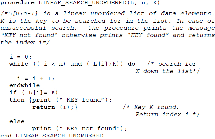
Algorithm 16.2 Procedure for unordered linear search
16.3. Transpose sequential search
Also known as self organizing sequential search, transpose sequential search searches a list of data items for a key, checking itself against the data items one at a time in a sequence. If the key is found, then it is swapped with its predecessor and the search is termed successful. The swapping of the search key with its predecessor, once it is found, favors a faster search when one repeatedly looks for the key. The more frequently one looks for a specific key in a list, the faster the retrievals take place in transpose sequential search since the found key moves towards the beginning of the list with every retrieval operation. Thus, a transpose sequential search is most successful when a few data items are repeatedly looked for in a list.
Algorithm 16.3 illustrates the working of transpose sequential search.


Algorithm 16.3 Procedure for transpose sequential search
Table 16.1 Transpose sequential search of {90, 89, 90, 21, 90, 90} in the list L= {34, 21, 89, 45, 12, 90, 76, 62}
| Search key | List L before search | Number of element comparisons made during the search | List L after search |
|---|---|---|---|
| 90 | {34, 21, 89, 45, 12, 90, 76, 62} | 6 | {34, 21, 89, 45, 90, 12, 76, 62} |
| 89 | {34, 21, 89, 45, 90, 12, 76, 62} | 3 | {34, 89, 21, 45, 90, 12, 76, 62} |
| 90 | {34, 89, 21, 45, 90, 12, 76, 62} | 5 | {34, 89, 21, 90, 45, 12, 76, 62} |
| 21 | {34, 89, 21, 90, 45, 12, 76, 62} | 3 | {34, 21, 89, 90, 45, 12, 76, 62} |
| 90 | {34, 21, 89, 90, 45, 12, 76, 62} | 4 | {34, 21, 90, 89, 45, 12, 76, 62} |
| 90 | {34, 21, 90, 89, 45, 12, 76, 62} | 3 | {34, 90, 21, 89, 45, 12, 76, 62} |
Transpose sequential search proceeds to find each key by the usual process of checking it against each element of L one at a time. However, once the key is found it is swapped with its predecessor in the list. Table 16.1 illustrates the number of comparisons made for each key during its search. The list L before and after the search operation are also illustrated in the table. The swapped elements in the list L after the search key is found is shown in bold. Observe how the number of comparisons made for the retrieval of 90 which is repeatedly looked for in the search list, decreases with each search operation.
The worst case complexity in terms of comparisons for finding a specific key in the list L is O(n). In the case of repeated searches for the same key, the best case would be O(1).
16.4. Interpolation search
Some search methods employed in every day life can be interesting. For example, when one looks for the word “beatitude” in the dictionary, it is quite common for one to turn over pages occurring at the beginning of the dictionary, and when one looks for “tranquility”, to turn over pages occurring towards the end of the dictionary. Also, it needs to be observed how during the search we turn sheaves of pages back and forth, if the word that is looked for occurs before or beyond the page that has just been turned. In fact, one may look askance at anybody who ‘dares’ to undertake sequential search to look for “beatitude” or “tranquility” in a dictionary!
Interpolation search is based on this principle of attempting to look for a key in a list of elements, by comparing the key with specific elements at “calculated” positions and ensuring if the key occurs “before” it or “after” it until either the key is found or not found. The list of elements must be ordered and we assume that they are uniformly distributed with respect to requests.
Let us suppose we are searching for a key K in a list L = {K1, K2, K3,…Kn}, K1 < K2 < … Kn of numerical elements. When it is known that K lies between Klow and Khigh, that is, Klow < K < Khigh, then the next element that is to be probed for key comparison is chosen to be the one that lies ![]() of the way between Klow and Khigh. It is this consideration that has made the search be termed interpolation search.
of the way between Klow and Khigh. It is this consideration that has made the search be termed interpolation search.
During the implementation of the search procedure, the next element to be probed in a sub list {Ki, Ki+1, Ki+2,…Kj} for comparison against the key K is given by Kmid where mid is given by ![]() . The key comparison results in any one of the following cases:
. The key comparison results in any one of the following cases:
If (K = Kmid) then the search is done.
If (K < Kmid) then continue the search in the sublist {Ki, Ki+1, Ki+2,…Kmid−1}.
If (K > Kmid) then continue the search in the sublist {Kmid+1, Kmid+2, Kmid+3, … Kj}.
Algorithm 16.4 illustrates the interpolation search procedure.
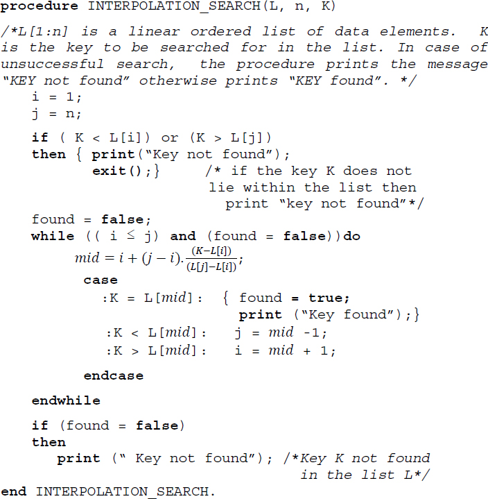
Algorithm 16.4 Procedure for interpolation search
Table 16.2 Trace of Algorithm 16.4 during the search for keys 67 and 45
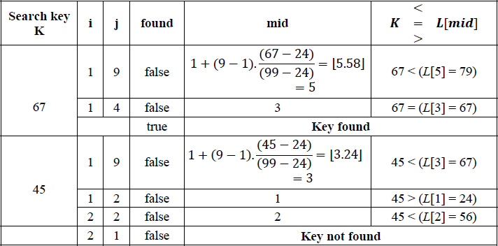 |
In the case of key 67, the search was successful. However in the case of key 45, as can be observed in the last row of the table, the condition (i ≤ j), that is, (2 ≤ 1) failed in the while loop of the algorithm and hence the search terminates signaling “Key not found”.
The worst case complexity of interpolation search is O(n). However, on average the search records a brilliant O(log2 log2 n) complexity.
16.5. Binary search
In the previous section we discussed interpolation search which works on ordered lists and reports an average case complexity of O(log2 log2 n). Another efficient search technique that operates on ordered lists is the binary search also known as logarithmic search or bisection.
A binary search searches for a key K in an ordered list L = {K1, K2, K3,…Kn}, K1 < K2 < … Kn of data elements, by halving the search list with each comparison until the key is either found or not found. The key K is first compared with the median element of the list, for example, Kmid. For a sublist {Ki, Ki+1, Ki+2, … Kj}, Kmid is obtained as the key occurring at the position mid which is computed as ![]() . The comparison of K with Kmid yields the following cases:
. The comparison of K with Kmid yields the following cases:
If (K = Kmid) then the binary search is done.
If (K < Kmid) then continue binary search in the sub list {Ki, Ki+1, Ki+2, … Kmid−1}.
If (K > Kmid) then continue binary search in the sub list {Kmid+1, Kmid+2, Kmid+3, … Kj}.
During the search process, each comparison of key K with Kmid of the respective sub lists results in the halving of the list. In other words, with each comparison the search space is reduced to half its original length. It is this characteristic that renders the search process efficient. Contrast this with a sequential list where the entire list is involved in the search!
Binary search adopts the Divide and Conquer method of algorithm design. Divide and Conquer is an algorithm design technique where to solve a given problem, the problem is first recursively divided (Divide) into sub problems (smaller problem instances). The sub problems that are small enough are easily solved (Conquer) and the solutions are combined to obtain the solution to the whole problem. Divide and Conquer has turned out to be a successful algorithm design technique with regard to many problems. Chapter 19 details the Divide and Conquer method of algorithm design.
In the case of binary search, the divide-and-conquer aspect of the technique breaks the list (problem) into two sub lists (sub problems). However, the key is searched for only in one of the sub lists hence with every division a portion of the list gets discounted.
Algorithm 16.5 illustrates a recursive procedure for binary search.
16.5.1. Decision tree for binary search
The binary search for a key K in the ordered list L = {K1, K2, K3,…Kn}, K1 < K2 < … Kn traces a binary decision tree. Figure 16.1 illustrates the decision tree for n = 15. The first element to be compared with K in the list L = {K1, K2, K3,…K15} is K8, which becomes the root of the decision tree. If K < K8 then the next element to be compared is K4, which is the left child of the decision tree. For the other cases of comparisons, it is easy to trace the tree by making use of the following characteristics:
i) The indexes of the left and the right child nodes differ by the same amount from that of the parent node
For example, in the decision tree shown in Figure 16.1 the left and right child nodes of the node K12, for example, K10 and K14 differ from their parent key index by the same amount.
This characteristic renders the search process to be uniform and therefore binary search is also termed as uniform binary search.
ii) For n elements where n = 2i − 1, the difference in the indexes of a parent node and its child nodes follows the sequence 20, 21, 22… from the leaf upwards.
For example, in Figure 16.1 where n = 15 = 24-1, the difference in index of all the leaf nodes from their respective parent nodes is 20. The difference in index of all the nodes in level 3 from their respective parent nodes is 21 and so on.
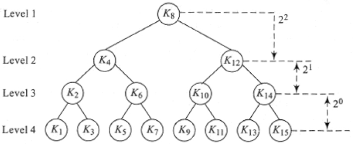
Figure 16.1 Decision tree for binary search
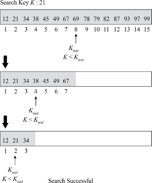
Figure 16.2 Binary search process (Example 16.5)
Let us now search for the key K = 75. Proceeding in a similar manner, K is first compared with K8 = 69. Since K > K8, the search list is reduced to {78, 79, 82, 87, 93, 97, 99}. Now K < (K12 = 87), hence the search list is reduced further to {78, 79, 82}. Comparing K with K10 reduces the search list to {78} which obviously yields the search to be unsuccessful.
In the case of Algorithm 16.5, at this step of the search, the recursive call to BINARY_SEARCH would have both low = high = 9, resulting in mid = 9. Comparing K with Kmid results in the call to binary_search(L, 9, 8, K). Since (low > high) condition is satisfied, the algorithm terminates with the ‘Key not found’ message.
Considering the decision tree associated with binary search, it is easy to see that in the worst case the number of comparisons needed to search for a key would be determined by the height of the decision tree and is therefore given by O(log2 n).
16.6. Fibonacci search
The Fibonacci number sequence is given by {0, 1, 1, 2, 3, 5, 8, 13, 21,…..} and is generated by the following recurrence relation:

It is interesting to note that the Fibonacci sequence finds an application in a search technique termed Fibonacci search. While binary search selects the median of the sub list as its next element for comparison, the Fibonacci search determines the next element of comparison as dictated by the Fibonacci number sequence.
Fibonacci search works only on ordered lists and for convenience of description we assume that the number of elements in the list is one less than a Fibonacci number, that is, n = Fk − 1. It is easy to follow Fibonacci search once the decision tree is traced, which otherwise may look mysterious!
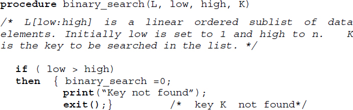
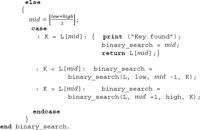
Algorithm 16.5 Procedure for binary search
16.6.1. Decision tree for Fibonacci search
The decision tree for Fibonacci search satisfies the following characteristics:
If we consider a grandparent, parent and its child nodes and if the difference in index between the grandparent and the parent is Fk then:
- if the parent is a left child node then the difference in index between the parent and its child nodes is Fk-1, whereas;
- if the parent is a right child node then the difference in index between the parent and the child nodes is Fk-2.
Let us consider an ordered list L = {K1, K2, K3,…Kn}, K1 < K2 < … Kn where n = Fk − 1. The Fibonacci search decision tree for n = 20 where 20 = (F8 -1) is shown in Figure 16.3.
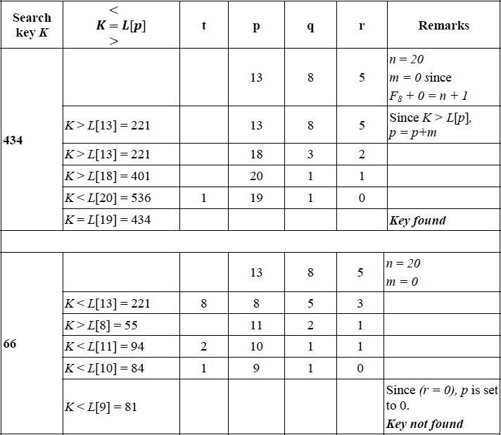
The root of the decision tree which is the first element in the list to be compared with key K during the search is that key Ki whose index i is the closest Fibonacci sequence number to n. In the case of n = 20, K13 is the root since the closest Fibonacci number to n = 20 is 13.
If (K < K13) then the next key to be compared is K8. If again (K < K8) then it would be K5 and so on. Now it is easy to determine the other decision nodes making use of the characteristics mentioned above. Since child nodes differ from their parent by the same amount, it is easy to see that the right child of K13 should be K18 and that of K8 should be K11 and so on. Consider the grandparent-parent combination, K8 and K11, respectively, since K11 is the right child of its parent and the difference between K8 and K11 is F4, the same between K11 and its two child nodes should be F2 which is 1. Hence the two child nodes of K11 are K10 and K12. Similarly, considering the grandparent and parent combination of K18 and K16 where K16 is the left child of its parent and their difference is given by F3, the two child nodes of K16 are given by K15 and K17 (difference is F2), respectively.

Figure 16.3 Decision tree for Fibonacci search
Algorithm 16.6 illustrates the procedure for Fibonacci search. Here n, the number of data elements is such that:
- Fk+1 > (n+1); and
- Fk + m = (n +1) for some m ≥ 0, where Fk+1 and Fk are two consecutive Fibonacci numbers.
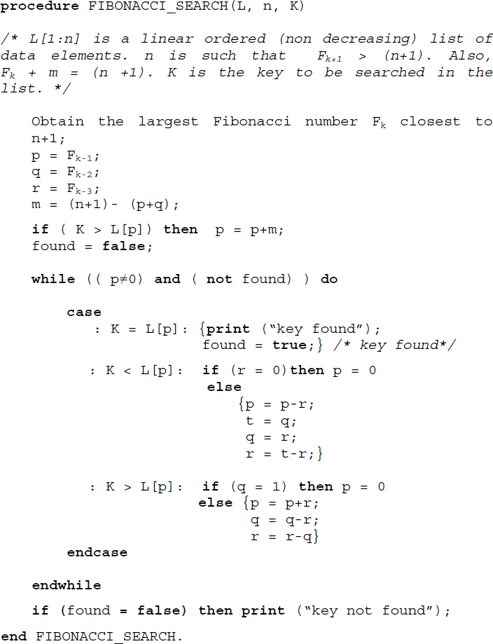
Algorithm 16.6 Procedure for Fibonacci search
16.7. Skip list search
Skip lists, invented in 1990 by Bill Pugh (Pugh 1990), are a good data structure for a dictionary ADT, which supports the operations of insert, delete and search. An ordered list of keys represented as a linked list would require O(n) time on an average, while searching for a key K. The search proceeds sequentially from the beginning of the list following the links one after another, until key K is found in the event of a successful search. Thus, there is no provision for a search to fast-forward itself, by skipping elements in the list and thereby speeding up search, before it finds key K or otherwise.
Table 16.3 Trace of Algorithm 16.6 (FIBONACCI SEARCH) for the search keys 434 and 66
 |
Skip lists, on the other hand, build layers of lists above the original list of keys, comprising selective keys from the original list, which act as “express lanes” for the keys in the immediately lower list, while searching for a key K. Each list in the layers has a header node and a sentinel node to signal the beginning and end of the list and comprises an ordered set of selective keys as nodes. The lower most list is the complete list of ordered keys in the original list, opening with a head node and ending with a sentinel node.
While searching for a key K in the list of keys, skip list search begins from the head node of the top most layer of the list, moving horizontally across the “express lane” comparing key K with the nodes in the list and stopping at a node whose next node has a key value greater than or equal to K. If the next node value equals K then the search is done. If not, the search drops down to the node in the immediate lower layer of the list, right underneath its present position, once again moving horizontally through the lower “express lane” looking for a node whose next node is greater than or equal to K. Eventually, if the key K did not match any of the nodes in the higher layers, then following the same principle of dropping down, the search finally reaches the original list of ordered keys in the lowermost layer and after a short sequential search, will find key K if it is successful search or would not find K in the case of unsuccessful search.
If S0 is the lowest layer comprising the original list of key values K1, K2, K3,…Kn, and S1, S2 … Sh are the higher layers of lists which act as “express lanes”, then the height of the skip list is h. Also, to favor comparison of node values with key K as the search progresses through the layers, it would be prudent to set the header node and sentinel node values of each list in the layers, to -∞ and +∞, respectively.
The selective nodes in the layers S1, S2 … Sh are randomly selected, quite often governed by a probability factor of ½ associated with the flipping of a coin! To build layer Si, each node entry in layer Si-1 after it makes its appearance in layer Si-1, flips a coin as it were and if it is “heads”, includes the same node entry in layer Si as well, and if it is “tails” discards making the entry in layer Si. The replication of node entries from lower layers to higher layers continues so long as the randomization process continues to flip “heads” for each layer. The moment the randomization process flips “tails” in any one of the layers, the replication of the node entries in the higher layer is stopped.
The skip list therefore can be viewed as a data structure with layers and towers, where each tower comprises replicated data entries over layers. In other words, a tower is made up of a single data value that is replicated across layers and therefore has different links to its predecessor and successor in each of the layers. If the lower most layer S0 had n node entries, then layer S1 could be expected to have n/2 node entries, layer S2 to have n/22 entries, generalizing, layer i could be expected to have n/2i node entries. In such a case, the height of the skip list could be expected to be O(log n). The average case time complexity of search in a skip list constructed such as this is, therefore, O(log n).
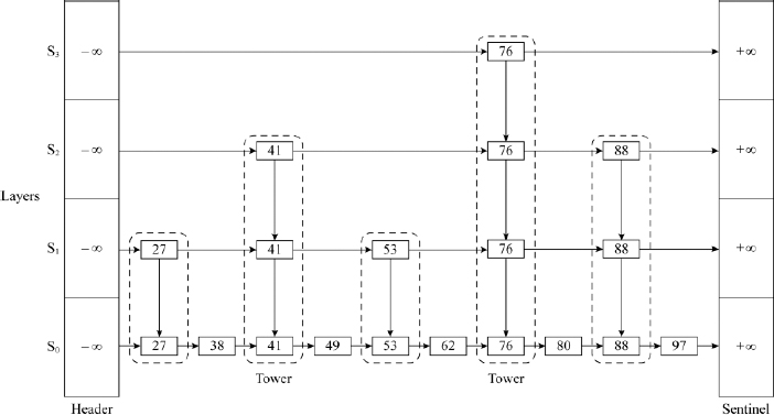
Figure 16.4 An example skip list with an illustrative structure, for searching a key K
To search for key K = 97, the procedure begins from the header node of layer S3 and stops at node 76 since the next node which is the sentinel node has a value +∞, which is greater than K. Thus, the search has moved through the S3 “express lane” skipping all the elements in the list whose value is less than 76. The search now descends to layer S2 and proceeds horizontally from node 76 until it stops at node 88. The search again descends to layer S1 and unable to proceed further horizontally stops at node 88 and descends one last time to layer S0. In layer S0, it moves horizontally from node 88, undertaking a sequential search and finds key K = 97 in the very next node. Thus, had it been an ordinary linked list, searching for key K should have taken 10 comparisons. On the other hand, the given skip list was able to fast track search and retrieve the key in half the number of comparisons.
To search for K = 53, the procedure begins from the header node of layer S3 and stops at the header node since the next node holds a value 76 which is greater than K. The search descends to the layer S2 and beginning with the header node, moves horizontally until it stops itself at node 41. The search descends to layer S1 and proceeds to move horizontally from node 41. The next node 53 is equal to key K and hence the search successfully terminates in layer S1 itself.
16.7.1. Implementing skip lists
The skip list diagram shown in Figure 16.4 is only illustrative of its structure. A skip list, in reality, could be implemented using a variety of ways innovated over a linked data structure. A straightforward implementation could call for a multiply-linked data structure to facilitate forward and backward, upward and downward movements. The availability of functions such as next(p), previous(p), above(p) and below(p), where p is the current position in the skip list, to undertake forward, backward, upward and downward movements, respectively, can help manage the operations of insert, delete and retrieval on a skip list. Alternate representations could involve opening variable sized nodes for each of the layers or opening nodes with a distinct node structure for the towers in the skip list and so on.
Algorithm 16.7 illustrates the search procedure on a skip list S for a key K. The algorithm employs functions next(p) and below(p) to undertake the search.
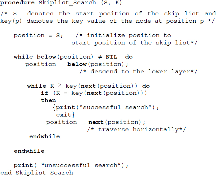
Algorithm 16.7 Procedure for skip list search
16.7.2. Insert operation in a skip list
To insert a key K into a skip list S, the procedure begins as if it were trying to search for a key K in the skip list S. Since the search would be unsuccessful, the lower most layer S0 which holds the original linked list of entries and most importantly the position where the key K needs to be inserted would be automatically arrived at since the condition K ≥ key(next(position))would have failed at that point. A new node with key K is inserted at that position. However, the problem does not end there.
It needs to be decided if the node K will find a place in the upper layers S1, S2, S3 and so forth, using randomization. Using the analogy of flipping a coin to illustrate randomization, “Heads” could mean insert K in the upper layer and “Tails” could mean discard insertion of key K in the upper layer as well in those above. If K is inserted in a higher layer, the randomization process continues to decide if it can be inserted in the next higher layer and so on, until a decision based on “Tails” discards its insertion in the next layer and above, once and for all. As can be observed, successive insertions of a key K in the upper layers of the skip list beginning with S0, in the event of a sequence of “Heads” decisions, results in building a tower for key K. The average time complexity of an insert operation in a skip list is O(log n).
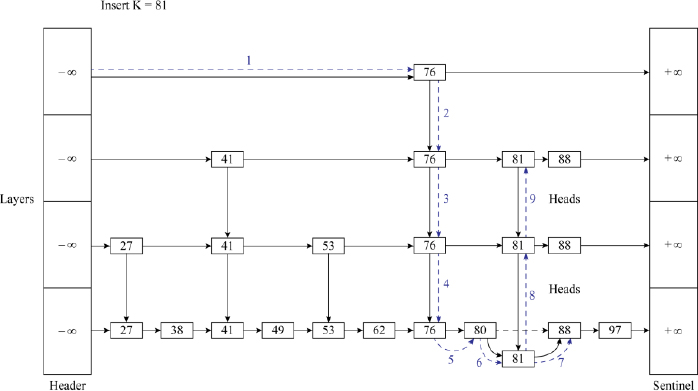
Figure 16.5 Insertion of key K = 81 in the skip list shown in Figure 16.4
16.7.3. Delete operation in a skip list
The delete operation on a skip list is easier than an insert operation. To delete key K, which let us assume is available in the skip list, the procedure proceeds as if it were searching for key K. Key K may be found in the top most layer of its tower if such a tower was built during the insertion of key K or may only be found in layer S0 as a node, in the absence of a tower.
In the case of a tower existing for key K, deletion only means deleting each of the nodes in its tower while moving downwards and appropriately resetting the links of its predecessor nodes to point to its successor nodes in all the layers covered by the tower. In the absence of a tower, it merely calls for deleting a single node in layer S0 and appropriately resetting the link of its predecessor node to point to its successor node. The average time complexity of a delete operation in a skip list is O(log n).
16.8. Other search techniques
16.8.1. Tree search
The tree data structures of AVL trees (section 10.3 of Chapter 10, Volume 2), m-way search trees, B trees and tries (Chapter 11, Volume 2), Red-Black trees (section 12.1 of Chapter 12, Volume 2) and so forth, are also candidates for the solution of search-related problems. The inherent search operation that each of these data structures support can be employed for the problem of searching.
The techniques of sequential search, interpolation search, binary search and Fibonacci search are primarily employed for files or groups of records or data elements that can be accommodated within the high speed internal memory of the computer. Hence, these techniques are commonly referred to as internal searching methods. On the other hand, when the file size is too large to be accommodated within the memory of the computer one has to take recourse to external storage devices such as disks or drums to store the file (Chapter 14). In such cases when a search operation for a key needs to be undertaken, the process involves searching through blocks of storage spanning across storage areas. Adopting internal searching methods for these cases would be grossly inefficient. The search techniques as emphasized by m-way search trees, B trees, tries and so on are suitable for such a scenario. Hence, these search techniques are referred to as external searching methods.
16.8.2. Graph search
The graph data structure and its traversal techniques of Breadth first traversal and Depth first traversal (section 9.4 of Chapter 9, Volume 2) can also be employed for search-related problems. If the search space is represented as a graph and the problem involves searching for a key K which is a node in the graph, any of the two traversals may be undertaken on the graph to look for the key. In such a case we term the traversal techniques as Breadth first search (see illustrative problem 16.6) and Depth first search (see illustrative problem 16.7).
16.8.3. Indexed sequential search
The indexed sequential search (section 14.7 of Chapter 14) is a successful search technique applicable on files that are too large to be accommodated in the internal memory of the computer. Also known as the Indexed Sequential Access Method (ISAM), the search procedure and its variants have been successfully applied to database systems.
Considering the fact that the search technique is commonly used on databases or files which span several blocks of storage areas, the technique could be deemed an external searching technique. To search for a key one needs to look into the index to obtain the storage block where the associated group of records or elements are available. Once the block is retrieved, the retrieval of the record represented by the key merely reduces to a sequential search within the block of records for the key.
Summary
- The problem of search involves retrieving a key from a list of data elements. In the case of a successful retrieval the search is deemed to be successful, otherwise unsuccessful.
- The search techniques that work on lists or files that can be accommodated within the internal memory of the computer are called internal searching methods, otherwise they are called as external searching methods.
- Sequential search involves looking for a key in a list L which may or may not be ordered. However, an ordered sequential search is more efficient than its unordered counterpart.
- A transpose sequential search sequentially searches for a key in a list but swaps it with the predecessor, once it is found. This enables efficient search of keys that are repeatedly looked for in a list.
- Interpolation search imitates the kind of search process that one employs while referring to a dictionary. The search key is compared with data elements at “calculated positions” and the process progresses based on whether the key occurs before or after it. However, it is essential that the list is ordered.
- Binary search is a successful and efficient search technique that works on ordered lists. The search key is compared with the element at the median of the list. Based on whether the key occurs before or after it, the search list is reduced and the search process continues in a similar fashion in the sub list.
- Fibonacci search works on ordered lists and employs the Fibonacci number sequence and its characteristics to search through the list.
- Skip lists are randomized and layered data structures that undertake search by skipping data elements through the list.
- Tree data structures, for example, AVL trees, tries, m-way search trees, B trees and so forth, and graphs also find applications in search-related problems. Indexed sequential search is a popular search technique employed in the management of files and databases.
16.9. Illustrative problems
Review questions
- Binary search is termed uniform binary search since its decision tree holds the characteristic of:
- the indexes of the left and the right child nodes differing by the same amount from that of the parent node;
- the list getting exactly halved in each phase of the search;
- the height of the decision tree being log2n;
- each parent node of the decision tree has two child nodes.
- In the context of binary search, state whether true or false:
- the difference in index of all the leaf nodes from their respective parent nodes is 20;
- the height of the decision tree is n
- true
- true
- true
- false
- false
- true
- false
- false
- For a list L = {K1, K2, K3, … K33}, K1 < K2 < … K33, undertaking Fibonacci search for a key K would yield a decision tree whose root node is given by:
- K16
- K17
- K1
- K21
- Which among the following search techniques does not report a worst case time complexity of O(n)?
- linear search
- interpolation search
- transpose sequential search
- binary search
- Which of the following search techniques works on unordered lists?
- Fibonacci search
- interpolation search
- transpose sequential search
- binary search
- What are the advantages of binary search over sequential search?
- When is a transpose sequential search said to be most successful?
- What is the principle behind interpolation search?
- Distinguish between internal searching and external searching.
- What are the characteristics of the decision tree of Fibonacci search?
- How is Breadth first search evolved from the Breadth first traversal of a graph?
- For the following search list undertake i) linear ordered search and ii) binary search of the data list given. Tabulate the number of comparisons made for each key in the search list.
Search list: {766, 009, 999, 238}
Data list: {111 453 231 112 679 238 876 655 766 877 988 009 122 233 344 566}
- For the given data list and search list, tabulate the number of comparisons made when i) a transpose sequential search and ii) interpolation search is undertaken on the keys belonging to the search list.
Data list:{pin, ink, pen, clip, ribbon, eraser, duster, chalk, pencil, paper, stapler, pot, scale, calculator}
Search list: {pen, clip, paper, pen, calculator, pen}
- Undertake Fibonacci search of the key K = 67 in the list {11, 89, 34, 15, 90, 67, 88, 01, 36, 98, 76, 50}. Trace the decision tree for the search.
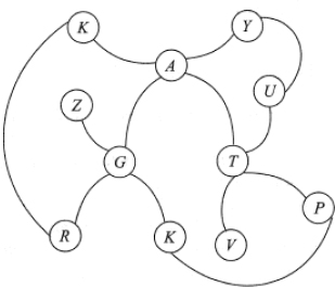
- Perform i) Breadth first search and ii) Depth first search, on the graph given below for the key V.
- A skip list is a:
- tree with ordered list of elements;
- binary search tree with unordered list of elements;
- a linked data structure that allows faster search with unordered elements;
- a linked data structure that allows faster search with ordered elements.
- Build a skip list for the following list of elements making your own assumptions on the randomization aspect.
10 40 50 70 80
- For the skip list constructed in review question 17, undertake the following operations:
- Delete 80
- Delete 10
Programming assignments
- Implement binary search and Fibonacci search algorithms (Algorithms 16.5 and 16.6) on an ordered list. For the list L = {2, 3, 4, 5, 6, 7, 8, 9, 10, 11, 12, 13, 14, 15, 16, 17, 18, 19, 20} undertake search for the elements in the list {3, 18, 1, 25}. Compare the number of key comparisons made during the searches.
- Execute an online dictionary (with a limited list of words) which makes use of interpolation search to search through the dictionary given a word. Refine the program to correct any misspelled word with the nearest and/or the correct word from the dictionary.
- L is a linear list of data elements. Implement the list as:
- a linear open addressed hash table using an appropriate hash function of your choice; and
- an ordered list.
Search for a list of keys on the representations i) and ii) using a) hashing and b) binary search, respectively. Compare the performance of the two methods over the list L.
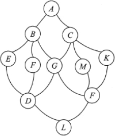
- Implement a procedure to undertake search for keys L and M in the graph shown below.
- Implement a menu-driven program to construct a skip list and search for keys available/unavailable in the list.